


1. Introduction
Waterflooding is a well-developed petroleum engineering technique used to increase oil recovery from hydrocarbon-bearing rocks (de Swaan Reference de Swaan1978; Weijermars, van Harmelen & Zuo Reference Weijermars, van Harmelen and Zuo2016). It relies on continuously pumping water over months or years in injector wells to drive the oil towards producer wells. The efficiency of water injection treatments to stimulate production is predicated in part on the initiation and propagation of hydraulic fractures at producer wells to ensure a more efficient sweep of the reservoir (van den Hoek & Mclennan Reference van den Hoek and Mclennan2000; Sharma et al. Reference Sharma, Pang, Wennberg and Morgenthaler2000; Noirot et al. Reference Noirot2003). This fracture allows the injected fluid to leak through the crack surfaces, which eventually leads to the development of a linear flow pattern around the borehole-fracture system.
The initiation of a hydraulic fracture is generally detected by a drop of the injection pressure, with the peak pressure referred to as the breakdown pressure. However, abnormally high peak pressure compared with the predicted fracture initiation pressure as well as unusually large time to reach the peak pressure have been observed in water flooding treatments of poorly consolidated rocks. These observations are counter-intuitive since the tensile strength should be so small in weak rocks that the breakdown pressure estimated according to the Haimson & Fairhurst (Reference Haimson and Fairhurst1967) criterion could in principle be approximated by the pressure required to reach an effective tensile hoop stress at the borehole wall.
It has been proposed that the abnormally high injection pressure is the result of a large apparent fracture toughness caused by yielding of the rock ahead of the crack (Papanastasiou & Thiercelin Reference Papanastasiou and Thiercelin1993; Papanastasiou Reference Papanastasiou1997, Reference Papanastasiou1999; van Dam, de Pater & Romijn Reference van Dam, de Pater and Romijn2000; van Dam, Papanastasiou & de Pater Reference van Dam, Papanastasiou and de Pater2002). However, laboratory fluid injection experiments in weak sandstone show evidence of injection-induced hairline cracks (Ispas et al. Reference Ispas, Eve, Hickman, Keck, Willson and Olson2012; Gao & Detournay Reference Gao and Detournay2020b), in contradiction with the blunt crack tip predicted by plasticity-based models (Germanovich et al. Reference Germanovich, Hurt, Ayoub, Siebrits, Norman, Ispas and Montgomery2012). This inconsistency between the plasticity hypothesis and the observed hairline cracks implies the existence of a different underlying mechanism behind the abnormally high injection pressure.
The theoretical model described in this paper suggests instead that the large peak pressure is linked to a transition of the flow pattern in the porous medium, caused by the moving boundary represented by the propagating crack.
The class of problems addressed here is actually quite different from the hydraulic fractures engineered to stimulate the production of oil and gas from a well. The key differences include: (i) the duration of the fluid injection phase (months or years instead of hours), (ii) the nature of the injected fluid (water instead of a high viscosity cake-building fluid), (iii) the range of strength and permeability of the host rock (strength of a few MPa and permeability in the range of  $0.1$ to $1$ Darcy instead of tens of MPa and permeability less than $10^{-2}$ Darcy).
Because of these fundamental differences between the two classes of problems, classical models of hydraulic fractures – the subject of intense research for several decades, see Adachi et al. (Reference Adachi, Siebrits, Peirce and Desroches2007), Detournay (Reference Detournay2016), and Lecampion, Bunger & Zhang (Reference Lecampion, Bunger and Zhang2018) for recent reviews – cannot be applied as such. In particular, the large-scale perturbation of the pore pressure and the related poroelastic effects cannot be ignored. Furthermore, in contrast to the classical hydraulic fracture models, the amount of fluid stored in the fracture is negligible compared with the volume of the fluid injected due to the high permeability; but it also should be neglected to avoid ill-conditioning of the equations. Finally, the borehole needs to be explicitly accounted for because the time-dependent partitioning of the fluid leakage between the borehole and the crack is an important element of the mechanism leading to a peak in the injection pressure.
This paper describes a two-dimensional (2-D) model of a hydraulic fracture within the particular context of waterflooding of weak, highly permeable rocks. It builds on our previous work on modelling fluid injection in a weak permeable rock within the context of a laboratory experiment (Gao & Detournay Reference Gao and Detournay2020a) and of a field test (Detournay & Hakobyan Reference Detournay and Hakobyan2021). Both studies have demonstrated that the peak pressure reflects a transition between two flow regimes. However, the model of a laboratory injection experiment was restricted to steady state in view of the smallness of the diffusion time scale compared with the experiment time scale in very permeable rocks. In that case, the fracture does not propagate unless the injection rate increases. On the other hand, the model for the field injection test neglects poroelasticity and the presence of the borehole, the latter affecting the asymptotic behaviour of the fluid partition between the borehole and the crack. Furthermore, the field model presented in that paper overlooked the existence of boundary layers that develop at the inlet and at the tip of the fracture under certain asymptotic conditions.
The paper is structured as follows. First the problem is formulated on the basis of the theories of poroelasticity, lubrication and linear elastic fracture mechanics. Taking advantage of the linearity of the equations of poroelasticity, the model is then reformulated as a nonlinear system of integro-differential equations, expressed in terms of variables that are only defined on the hydraulic fracture. A scaling analysis reveals that the system only depends on dimensionless time  $\tau$ and on two other parameters, the scaled borehole radius $\alpha _k$ and the poroelastic coefficient $\eta$. Three time asymptotic solutions are then analysed, small- and large-time asymptotes, as well as an intermediate-time asymptote that exists on the condition that $\alpha _{k}$ is small. The boundary layer at the crack inlet for the intermediate asymptote, and at the crack tip for the large-time asymptote are analysed. These boundary layers break locally the similarity nature of these asymptotic solutions. Discretization of the integro-differential system of equations leads to the formulation of a nonlinear system of algebraic equations, which is solved numerically for particular combinations of time $\tau$ and numbers $\alpha _{k}$ and $\eta$. Finally, application of the proposed model to waterflooding operations is discussed.
2. Mathematical model
2.1. Problem description
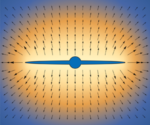
The waterflooding problem is analysed within the framework of the 2-D model sketched in figure 1. It consists of an infinite poroelastic domain with a circular hole of radius  $a$, constrained to deform under plane strain conditions and subjected to a far-field isotropic compressive stress $\sigma _{0}$ and a far-field pore pressure $p_{0}<\sigma _{0}$. The porous material is saturated by a Newtonian fluid. It is also assumed to be perfectly brittle but with a negligible toughness, i.e. $K_{Ic}=0$. There are six independent parameters to describe the Newtonian fluid and the poroelastic material, namely: dynamic viscosity $\mu$, Young's modulus $E$, Poisson's ratio $\nu$, Biot coefficient $\alpha$, permeability $k$ or mobility $\kappa =k/\mu$, and diffusivity $c$. Three derived parameters are introduced to simplify the problem formulation,
 \begin{equation} E'=\frac{E}{1-\nu^{2}},\quad \eta=\frac{\alpha(1-2\nu)}{2(1-\nu)},\quad \mu'=12\mu, \end{equation}
where  $E'$ denotes the plane strain Young's modulus, and $\eta \in [0,1/2]$ is a poroelastic stress coefficient (Detournay & Cheng Reference Detournay and Cheng1993).

Figure 1. (a) A schematic diagram of the bi-wing fracture near a borehole and (b) poroelastic medium  $\mathcal {D}$, wellbore $\mathcal {W}$ and bi-wing crack $\mathcal {C}$ with corresponding field variables.
With the hole initially filled by the same fluid at pressure  $p_{0}$, the system is initially equilibrated with a uniform pore pressure $p_{0}$. There is an initial elastic stress concentration at the hole boundary on account of the difference between the fluid pressure in the hole and the far-field stress. At time $t=0$, fluid is injected in the hole at a constant rate $Q_{0}$ (dimension $L^{2}T^{-1}$) causing a progressive change in the stress and pore pressure field in the vicinity of the hole that eventually lead to the initiation at the circular boundary of a symmetric bi-wing hydraulic fracture. The direction of fracture is associated with a small anisotropy of the far-field stress that causes the crack to propagate in the direction perpendicular to the least compressive far-field stress. Propagation of the fracture is tracked by the distance $\ell$ between the crack tip and the hole centre. This distance, a monotonic function of time $t$, will simply be referred to as the crack length.
The primary objective of the analysis is to determine the evolution of the borehole pressure  $p_{w}$ and the crack length $\ell$, as well as the dependence of the functions $p_{w}(t)$ and $\ell (t)$ on the various parameters describing this system.
2.2. Assumptions
The mathematical model is constructed on the following two critical hypotheses: (i) the crack propagates in a region surrounding the borehole, where the pore pressure field is quasi-steady; (ii) fluid storage in the crack is negligible compared with the amount of fluid lost by leak-off. The justification for these two hypotheses lays in the presumed large permeability of the rock, which is assumed to be poorly consolidated. Such a rock is also assumed to have a negligible fracture toughness.
As a consequence of the first hypothesis, the diffusion equation governing the evolution of the pore pressure field degenerates into a Laplace equation in a region containing the crack. This degeneracy transforms the two-way poroelastic coupling between the stress and pore pressure fields to a one-way coupling; i.e. the pore pressure field can be solved first, and then acts as a forcing term in the elasticity equation governing the stress field. Although the solution still depends on time, due to the far-field asymptotic solution of the diffusion equation, the combined hypotheses lead to a history-independent solution. In other words, time  $t$ becomes an independent parameter of the solution rather than a variable, as further discussed in § 3.3.
2.3. Field variables in Poroelastic domain  $\mathcal {D}$ and crack $\mathcal {C}$


A 2-D cartesian coordinates system  $(x,y)$ centred on the borehole is defined with the $x$-axis oriented along the crack. Two sub-domains are naturally introduced: the 2-D poroelastic domain $\mathcal {D}=\{(x,y)\,|\,x^{2}+y^{2}\geqslant a^{2}\}$ and the crack $\mathcal {C}=\{(x,y)\mid x\in [-\ell ,-a]\cup [a,\ell ], y=0\}$. Domain $\mathcal {D}$ is bounded by wellbore $\mathcal {W}=\{(x,y)\,|\,x^{2}+y^{2}=a^{2}\}$ and crack $\mathcal {C}$. The field variables defined on $\mathcal {D}$ are stress $\boldsymbol {\boldsymbol {\sigma }}$, displacement $\boldsymbol {\boldsymbol {u}}$, pore pressure $p$ and specific discharge $\boldsymbol {\boldsymbol {v}}$. On $\mathcal {C}$, the field variables are fluid pressure $p_{f}$, leak-off $g$, crack aperture $w$ and flux $q$. All these variables are functions of time $t$. The variables are constrained by the following continuity and jump conditions between the two sub-domains:
 \begin{equation} \left.\begin{gathered} p_{f}(x,t)=p(x,0,t),\quad p_{f}(x,t)={-}\sigma_{yy}(x,0,t),\quad \sigma_{xy}(x,0,t)=0,\\ w(x,t)=[{u_{y}(x,0,t)]},\quad g(x,t)=[{v_{y}(x,0,t)]}. \end{gathered}\right\} \end{equation}
Here  $a< | x| < \ell$, and $[ {f(x,0,t)]}\equiv f(x,0^{+},t)-f(x,0^{-},t)$.
The field variables in  $\mathcal {D}$ are governed by the theory of poroelasticity, while those in $\mathcal {C}$ are also governed by the lubrication equation and by the fracture propagation criterion. The complete set of governing equations and boundary conditions are presented in §§ 2.4–2.7.
2.4. Governing equations on $\mathcal {D}$

The equations of poroelasticity can be reduced to a set of two coupled partial differential equations that govern the displacement field  $\boldsymbol {\boldsymbol {u}}(\boldsymbol {\boldsymbol {x}},t)$ in the porous solid and the pore pressure field $p(\boldsymbol {\boldsymbol {x}},t)$: namely, a Navier-type equation for $\boldsymbol {\boldsymbol {u}}(\boldsymbol {\boldsymbol {x}},t)$ with a body force term proportional to the pore pressure gradient, and a diffusion equation for $p(\boldsymbol {\boldsymbol {x}},t)$ with a source term proportional to the rate of change of $\boldsymbol {\nabla }\boldsymbol {\cdot }\boldsymbol {\boldsymbol {u}}$ (Cheng Reference Cheng2016). The coupling term in the diffusion equation vanishes, however, when the solution reaches a steady state or when the displacement field is irrotational and the medium is infinite (Detournay & Cheng Reference Detournay and Cheng1993). As elaborated in more details in § 3.1, the first condition is indeed met in the problem in view of the a priori hypothesis that the crack is growing in a region where the flow is in a pseudo steady-state.
Thus, in the near-field the pore pressure is governed by Laplace equation
 \begin{equation} \kappa\nabla^{2}p={-}g(x,t)\delta(y), \end{equation}
where  $\delta (y)$ denotes the Dirac delta function, and the leak-off $g(x,t)$ is part of the solution. While in the far field, $p(x,t)$ is given by the solution of
 \begin{equation} \frac{\partial p}{\partial t}-c\nabla^{2}p=Q_{0}\delta(\boldsymbol{\boldsymbol{x}})H(t), \end{equation}
where  $H(t)$ is the Heaviside function. This asymptotic solution actually corresponds to the classical continuous source solution (Cheng Reference Cheng2016). The specific discharge $\boldsymbol {\boldsymbol {v}}$ is related to the pore pressure $p$ according to Darcy's law
 \begin{equation} \boldsymbol{\boldsymbol{v}}={-}\kappa\boldsymbol{\nabla} p. \end{equation}
 The Navier equation for the displacement  $\boldsymbol {\boldsymbol {u}}$ is given by
 \begin{equation} G\nabla^{2}\boldsymbol{\boldsymbol{u}}+\frac{G}{1-2\nu}\boldsymbol{\nabla}(\boldsymbol{\nabla}\boldsymbol{\cdot}\boldsymbol{\boldsymbol{u}})-\alpha\boldsymbol{\nabla} p=0, \end{equation}
where  $G=E/2(1+\nu )$ is the shear modulus. The stress $\boldsymbol {\boldsymbol {\sigma }}$ is related to pore pressure $p$ and strain $\boldsymbol {\boldsymbol {\varepsilon }}=(\boldsymbol {\nabla }\boldsymbol {\boldsymbol {u}}+\boldsymbol {\boldsymbol {u}}\boldsymbol {\nabla })/2$ according to
 \begin{equation} \boldsymbol{\boldsymbol{\sigma}}+\alpha p\boldsymbol{\boldsymbol{I}}=2G\boldsymbol{\boldsymbol{\varepsilon}}+ \frac{2G\nu}{1-2\nu}(\boldsymbol{\boldsymbol{\varepsilon}}:\boldsymbol{\boldsymbol{I}})\boldsymbol{\boldsymbol{I}}, \end{equation}
where  $\boldsymbol {\boldsymbol {I}}$ denotes the second-order identity tensor.
The system (2.3)–(2.7) represent the complete set of equations governing the fields  $\boldsymbol {\boldsymbol {u}}(\boldsymbol {\boldsymbol {x}},t)$, $p(\boldsymbol {\boldsymbol {x}},t)$, $\boldsymbol {\boldsymbol {\sigma }}(\boldsymbol {\boldsymbol {x}},t)$, $\boldsymbol {\boldsymbol {v}}(\boldsymbol {\boldsymbol {x}},t)$ in $\mathcal {D}$.
2.5. Boundary conditions on $\mathcal {W}$

The injection pressure  $p_{w}$ and the fraction $(1-\varPhi$) of the injection rate $Q_{0}$ directly entering the rock through the borehole wall (to be discussed near (3.21)) are both a priori unknown functions of time $t$. The borehole pressure $p_{w}$ represents a boundary condition on wellbore $\mathcal {W}$ for both the stress and the pore pressure,
 \begin{equation} \boldsymbol{\boldsymbol{\sigma}}(\boldsymbol{\boldsymbol{x}},t)\boldsymbol{\cdot}\boldsymbol{\boldsymbol{n}}={-}p_{w}\boldsymbol{\boldsymbol{n}},\quad p(\boldsymbol{\boldsymbol{x}},t)=p_{w},\quad \boldsymbol{\boldsymbol{x}}\in\mathcal{W}, \end{equation}
where  $\boldsymbol {\boldsymbol {n}}$ denotes the unit normal external vector on $\mathcal {W}$. The rate of fluid volume passing through the borehole wall and the flux at the crack inlet are constrained by the total injection $Q_{0}$,
 \begin{equation} -\oint_{\mathcal{W}}\boldsymbol{\boldsymbol{v}}(\boldsymbol{\boldsymbol{x}},t)\boldsymbol{\cdot}\boldsymbol{\boldsymbol{n}}\,{\rm d} s+2q(a,t)=Q_{0}, \end{equation}
where the symmetry condition has been taken into account in (2.9).
2.6. Governing equations on $\mathcal {C}$

The equations governing the fluid flow in the crack  $\mathcal {C}$ are Poiseuille's law
 \begin{equation} q={-}\frac{w^{3}}{\mu'}\frac{\partial p_{f}}{\partial x}, \end{equation}
and the continuity equation
 \begin{equation} \frac{\partial q}{\partial x}+g=0, \end{equation}
with the storage term neglected in accord with the simplifying assumption stated earlier. Combining (2.11) and (2.10) yields the Reynolds lubrication equation
 \begin{equation} \frac{1}{\mu'}\frac{\partial}{\partial x}\left({w^{3}\frac{\partial p_{f}}{\partial x}}\right)=g. \end{equation}
Two additional boundary conditions are required for the lubrication equation. One condition imposes the pressure at the fracture inlet, and the other one a vanishing flux at the crack tip (Detournay & Peirce Reference Detournay and Peirce2014),
 $$\begin{gather} p_{f}({\pm} a,t)=p_{w}, \end{gather}$$
 $$\begin{gather}q({\pm}\ell(t),t)=0. \end{gather}$$
2.7. Tip asymptotics
According to linear elastic fracture mechanics (LEFM), the crack aperture asymptotically behaves near the advancing tip as
 \begin{equation} w(x)\propto(\ell- |x| )^{{3}/{2}},\quad x\to\pm\ell, \end{equation}
if the fracture toughness  $K_{Ic}=0$ and provided that the fluid pressure is finite at the tip. This latter condition is indeed fulfilled as the fluid pressure in the crack is continuous with the pore pressure field, which must be regular as it is governed by the Laplace equation in a finite region (Evans Reference Evans2010). (Since a 2-D point source leads to a logarithmically singular pore pressure, the pore pressure induced by a distributed leak-off at the crack tip is thus regular as can be confirmed by convolving the source function with the leak-off.) Hence, the fluid pressure $p_{f}$ at the tip can be expanded as
 \begin{equation} p_{f}(x)=c_{0}+c_{1}({\ell- |x| })+O ({\ell- |x| })^{2},\quad x\to\pm\ell, \end{equation}
which satisfies the requirement of the crack aperture tip asymptotic solution (2.15).
Substituting the above tip asymptotics for  $p_{f}$ and $w$ into the lubrication equation (2.12), shows that the leak-off $g$ near the tip should behave as
 \begin{equation} g\propto(\ell- |x| )^{{7}/{2}},\quad x\to\pm\ell. \end{equation}
 The tip asymptotic solution outlined above differs from tip asymptotic solutions for hydraulic fractures propagating in permeable media, constructed on the assumptions that leak-off is either governed by the one-dimensional Carter law (Lenoach Reference Lenoach1995; Garagash, Detournay & Adachi Reference Garagash, Detournay and Adachi2011; Detournay Reference Detournay2016) or by the diffusion equation (Detournay & Garagash Reference Detournay and Garagash2003). Solutions built on assuming Carter leak-off (Howard & Fast Reference Howard and Fast1957) predict  $p_{f}(x)$ to be singular (with the singularity depending on whether the fracture propagates in the viscosity- or the toughness-dominated regime) and leak-off rate to have a square root singularity. On the other hand, asymptotic solutions obtained on the basis of the diffusion equation require the existence of a lag region, which is filled by pore fluid circulating in and out of the cavity.
3. Method of solution
In view of the linearity of the governing equations in  $\mathcal {D}$, the field variables $\boldsymbol {\boldsymbol {\sigma }}$ and $p$ in $\mathcal {D}$ can be expressed as integrals of distributed singularities convolved with influence functions over the boundaries of $\mathcal {D}$. The detail of this method is discussed in this section, and further simplifications are adopted to reduce the integral on the crack boundary $\mathcal {C}$ only. In addition, due to the symmetry of the problem, only half of the crack $\tilde {\mathcal {C}}=\{(x,0)\mid a\leqslant x\leqslant \ell \}$ is required for the convolution integrals.
3.1. Pore pressure field
The pore pressure field is formulated as a superposition of three particular solutions, each satisfying the condition that the pore pressure on the borehole boundary  $\mathcal {W}$ is uniform,
 \begin{equation} p(x,y,t)=p_{0}+p_{i}(x,y,t)+p_{l}(x,y,t), \end{equation}
where  $p_{i}(x,y,t)$ is the pore pressure induced by continuous injection from the borehole in the absence of a fracture, and $p_{l}(x,y,t)$ the pore pressure field associated with leak-off from the fracture. The field $p_l$ does not contribute to the total flow rate entering the porous medium $\mathcal {D}$, as explained later.
The field  $p_{i}$ is given by the classical source solution of the diffusion equation (Carslaw & Jaeger Reference Carslaw and Jaeger1959)
 \begin{equation} p_{i}(x,y,t)=\frac{Q_{0}}{4{\rm \pi}\kappa}E_{1}\left({\frac{r^{2}}{4ct}}\right). \end{equation}
Inside the quasi-stationary region which expands as  $\chi \sqrt {ct}$, the diffusion equation effectively degenerates to Laplace equation (2.3). In this region the exponential integral function $E_1$ simplifies to (Abramowitz & Stegun Reference Abramowitz and Stegun1972)
 \begin{equation} p_{i}(x,y,t)\approx{-}\frac{Q_{0}}{2{\rm \pi}\kappa}\left({\ln\frac{r}{2\sqrt{ct}}+\frac{\gamma}{2}}\right),\quad r<\chi\sqrt{ct}, \end{equation}
with  $r=\sqrt {x^{2}+y^{2}}$ and $\gamma =0.577216\cdots$ denoting the Euler gamma constant. The number $\chi \approx 0.35$ defines the conditions for which the asymptotic solution (3.3) applies within an error less than 1 %.
The field  $p_{l}(x,y,t)$ breaks the axial symmetry of the injection-induced pore pressure $p_{i}(x,y,t)$ by accounting for leak-off from the fracture. This field, which is also assumed to satisfy the Laplace equation, is constructed by distributing fluid sources along the crack $\mathcal {C}$ and image sinks inside the borehole $\mathcal {W}$ so that there is no net fluid injection in the poroelastic media $\mathcal {D}$. The locations of the image sinks inside $\mathcal {W}$ are chosen so that the pore pressure $p_{l}$ is uniform on $\mathcal {W}$. Thus, the field $p_{l}(x,y,t)$ is expressed as a convolution integral of the leak-off $g$ with the singular kernel $\tilde {P}(x,y,s,a)$ (Gao & Detournay Reference Gao and Detournay2020a), i.e.
 \begin{equation} p_{l}(x,y,t)=\frac{1}{2{\rm \pi}\kappa}\int_{a}^{\ell}g(s,t)\tilde{P}(x,y,s,a)\,{\rm d}s. \end{equation}
The kernel  $\tilde {P}(x,y,s,a)$ accounts for the problem symmetry with respect to the $y$-axis by taking the form
 \begin{equation} \tilde{P}(x,y,s,a)=P(x,y,s,a)+P({-}x,y,s,a), \end{equation}
with  $P$ representing the pore pressure field generated by a source located at $(s,0)$ and an image sink positioned at $(a^{2}/s,0)$, $s>a$. On $y=0$, the kernel $P$ is simply given by
 \begin{equation} P(x,0,s,a)={-}\ln |x-s|+\ln \left| {x-\frac{a^{2}}{s}}\right| . \end{equation}
Expression (3.4) for the pore pressure field  $p_{l}$ ensures that there is no contribution from this field to the total flow rate entering the domain in $\mathcal {D}$. In other words,
 \begin{equation} \oint_{\mathcal{W}}\boldsymbol{\boldsymbol{v}}_{l}\boldsymbol{\cdot}\boldsymbol{\boldsymbol{n}}\,{\rm d}s=2q(a,t). \end{equation}
With the introduction of the image sink, the same flux entering the fracture inlet is coming back through the borehole boundary  $\mathcal {W}$, so that $(1-\varPhi )Q_0$ is leaking through $\mathcal {W}$ and $\varPhi Q_0$ through the walls of crack $\mathcal {C}$. After superposing all the fields, the rate of fluid volume injected into the media is $Q_0$. Here $\varPhi$ denotes the fraction of injected fluid leaking through $\mathcal {C}$; an expression to calculate $\varPhi$ is given in (3.21).
In summary, the pore pressure field induced by injection  $Q_{0}$ and leak-off $g$ is found by combining (3.1), (3.2) and (3.4). On the crack ( $a\leqslant |x| \leqslant \ell , y=0$) the fluid pressure reads as
 \begin{equation} p_{f}(x,t)=p_{0}-\frac{Q_{0}}{2{\rm \pi}\kappa}\left( {\ln\frac{ |x| }{2\sqrt{ct}} + \frac{\gamma}{2}}\right)+\frac{1}{2{\rm \pi}\kappa}\int_{a}^{\ell}g(s,t)\tilde{P}(x,0,s,a)\,{\rm d}s. \end{equation}
To simplify the notation, the second parameter of  $\tilde {P}$ is omitted in the rest of the paper, if it is zero, i.e. $\tilde {P}(x,s,a)\equiv \tilde {P}(x,0,s,a)$.
3.2. Stress field
Taking advantage of the linearity of the elasticity equations (2.6) and (2.7), the stress field  $\boldsymbol {\boldsymbol {\sigma }}$ in $\mathcal {D}$ can also be constructed by superposition of particular solutions. Here, only the stress $\sigma _{yy}$ on the crack $\mathcal {C}$ is of concern; it is decomposed into four parts: (i) the in-situ stress $-\sigma _{0}$, (ii) the stress $\sigma _{yy}^{f}$ induced by the crack aperture $w$, (iii) the poroelastic stress $\sigma _{yy}^{p}$ induced by the pore pressure change $p-p_{0}$, and (iv) a stress $\sigma _{yy}^{c}$ resulting from enforcing the stress boundary condition (2.8a). Thus,
 \begin{equation} \sigma_{yy}(x,0,t)={-}\sigma_{0}+\sigma_{yy}^{f}+\sigma_{yy}^{p}+\sigma_{yy}^{c}. \end{equation}
 The crack induced stress  $\sigma _{yy}^{f}$ can be expressed as (Hills et al. Reference Hills, Kelly, Dai and Korsunsky1996)
 \begin{equation} \sigma_{yy}^{f}(x,t)=\frac{E'}{4{\rm \pi}}\int_{a}^{\ell}w(s,t)\frac{\partial}{\partial s}\tilde{H}(x,s,a)\,{\rm d}s, \end{equation}
where
 \begin{equation} \tilde{H}(x,s,a)\equiv H(x,s,a)+H({-}x,s,a), \end{equation}
noting also that  $\tilde {H}(x,a,a)=0$ and $w(\ell )=0$. The kernel function $H(x,s,a)$,
 \begin{align} H(x,s,a) &= \frac{s^{2}-a^{2}}{sx^{2}}-\frac{a^{2}\left(s^{2}-a^{2}\right)}{s\left(sx-a^{2}\right)^{2}} \left(\frac{s^{2}}{a^{2}}-\frac{s^{2}-a^{2}}{sx-a^{2}}\right) \nonumber\\ &\quad -\frac{s}{sx-a^{2}}+\frac{a^{2}}{x^{3}}+\frac{1}{x-s}+\frac{1}{x}, \end{align}
represents the stress  $\sigma _{yy}(x,0)$ induced by a unit normal dislocation located at $(s,0)$ along the $y$-axis that satisfies the boundary condition $\boldsymbol {\boldsymbol {\sigma }}\boldsymbol {\cdot }\boldsymbol {\boldsymbol {n}}=0$ on borehole $\mathcal {W}$ (Dundurs & Mura Reference Dundurs and Mura1964; Hills et al. Reference Hills, Kelly, Dai and Korsunsky1996).
Echoing the decomposition of  $p$ in § 3.1, the poroelastic stress $\boldsymbol {\boldsymbol {\sigma }}^{p}$ is expressed as the sum of an injection-induced stress $\boldsymbol {\boldsymbol {\sigma }}_{i}^{p}$ and the leak-off induced stress $\boldsymbol {\boldsymbol {\sigma }}_{l}^{p}$. On crack $\mathcal {C}$, $\boldsymbol {\boldsymbol {\sigma }}_{i}^{p}$ is given by (Cheng & Detournay Reference Cheng and Detournay1998; Gao & Detournay Reference Gao and Detournay2020a)
 \begin{equation} \left.\begin{gathered} \sigma_{xx,i}^{p}(x,0,t) ={-}2\eta\frac{Q_{0}}{4{\rm \pi}\kappa} \left[{-\frac{\gamma}{2}-\ln\frac{ |x|}{2\sqrt{ct}}+ \frac{1}{2}}\right]={-}\eta p_{i}(x,0,t)-\eta\frac{Q_{0}}{4{\rm \pi}\kappa},\\ \sigma_{yy,i}^{p}(x,0,t) ={-}2\eta\frac{Q_{0}}{4{\rm \pi}\kappa} \left[{-\frac{\gamma}{2}-\ln\frac{ |x| }{2\sqrt{ct}}- \frac{1}{2}}\right]={-}\eta p_{i}(x,0,t)+\eta\frac{Q_{0}}{4{\rm \pi}\kappa},\\ \sigma_{xy,i}^{p}(x,0,t) =0. \end{gathered}\right\} \end{equation}
 It can be shown, using the poroelastic steady-state source solution, that the leak-off induced stress  $\boldsymbol {\boldsymbol {\sigma }}_{l}^{p}$ on the crack $\mathcal {C}$ is given by (Gao & Detournay Reference Gao and Detournay2020a)
 \begin{equation} \sigma_{xx,l}^{p}(x,0,t)=\sigma_{yy,l}^{p}(x,0,t)={-}\eta p_{l}(x,0,t),\quad \sigma_{xy,l}^{p}(x,0,t)=0. \end{equation}
 Combining (3.13), (3.14a,b) and (3.1) leads to the following expressions for the induced normal and shear stresses  $\sigma _{yy}^{p}$ and $\sigma _{xy}^{p}$ on $\mathcal {C}$:
 \begin{equation} \sigma_{yy}^{p}(x,0)={-}\eta(p_{f}(x)-p_{0})+\eta\frac{Q_{0}}{4{\rm \pi}\kappa},\quad \sigma_{xy}^{p}(x,0)=0,\quad a\leqslant|x| \leqslant\ell. \end{equation}
 The normal and shear stresses  $\{\sigma _{rr}^{p},\sigma _{r\theta }^{p}\}$ acting on borehole boundary $\mathcal {W}$ need also to be evaluated to determine $\sigma _{yy}^{c}$ in (3.9), as shown below. While it is clear that the borehole injection-induced component $\boldsymbol {\boldsymbol {\sigma }}_{i}^{p}$ of $\boldsymbol {\boldsymbol {\sigma }}^{p}$ satisfies $\boldsymbol {\boldsymbol {\sigma }}_{i}^{p}(\boldsymbol {\boldsymbol {x}})\boldsymbol {\cdot }\boldsymbol {\boldsymbol {n}}=\sigma _{xx,i}^{p}(a,0)\boldsymbol {\boldsymbol {n}}$ on $\boldsymbol {\boldsymbol {x}}\in \mathcal {W}$, we assume that the leak-off induced normal stress on $\mathcal {W}$ is also uniform and given by $\boldsymbol {\boldsymbol {\sigma }}_{l}^{p}(\boldsymbol {\boldsymbol {x}})\boldsymbol {\cdot }\boldsymbol {\boldsymbol {n}}\approx \sigma _{xx,l}^{p}(a,0)\boldsymbol {\boldsymbol {n}}=-\eta p_{l}(a,0)\boldsymbol {\boldsymbol {n}}$ on $\boldsymbol {\boldsymbol {x}}\in \mathcal {W}$. With this assumption and (3.13), the expressions for $\sigma _{rr}^{p}$ and $\sigma _{r\theta }^{p}$ acting on $\mathcal {W}$ simplify to
 \begin{equation} \sigma_{rr}^{p}(\boldsymbol{\boldsymbol{x}})={-}\eta(p_{w}-p_{0})-\eta\frac{Q_{0}}{4{\rm \pi}\kappa},\quad \sigma_{r\theta}^{p}(\boldsymbol{\boldsymbol{x}})=0,\quad \boldsymbol{\boldsymbol{x}}\in\mathcal{W}. \end{equation}
The approximation adopted for  $\boldsymbol {\boldsymbol {\sigma }}_{l}^{p}$ recognizes that $\boldsymbol {\boldsymbol {\sigma }}_{l}^{p}$ is negligible compared with $\boldsymbol {\boldsymbol {\sigma }}_{i}^{p}$ for a short crack, as only a small portion of fluid is leaking from the crack; while for a long crack, the actual stress boundary conditions on borehole $\mathcal {W}$ are effectively irrelevant at the scale of the fracture.
Finally, the fourth term  $\sigma _{yy}^{c}$ in (3.9) is obtained by enforcing the boundary condition (2.8a). After considering the in-situ stresses $\sigma _0$ and the poroelasticity induced normal stress $\sigma _{rr}^{p}$ on borehole $\mathcal {W}$ in (3.16a), $\sigma _{yy}^{c}$ is given by (Cheng Reference Cheng2016)
 \begin{equation} \sigma_{yy}^{c}(x)=\left[{p_{w}-\sigma_{0}-\eta(p_{w}-p_{0})-\eta\frac{Q_{0}}{4{\rm \pi}\kappa}}\right]\frac{a^{2}}{x^{2}}. \end{equation}
 In summary, the normal stress  $\sigma _{yy}$ on crack $\mathcal {C}$ is obtained by substituting (3.10), (3.15a) and (3.17) into (3.9) to give
 \begin{align} \sigma_{yy}(x,0) &={-}\sigma_{0}+\left[{p_{w}-\sigma_{0}-\eta(p_{w}-p_{0})-\frac{\eta Q_{0}}{4{\rm \pi}\kappa}}\right] \frac{a^{2}}{x^{2}} \nonumber\\ &\quad -\eta(p_{f}(x)-p_{0})+\frac{\eta Q_{0}}{4{\rm \pi}\kappa}+\frac{E'}{4{\rm \pi}} \int_{a}^{\ell}w(s)\frac{\partial}{\partial s}\tilde{H}(x,s,a)\,{\rm d}s. \end{align}
3.2.1. Influence of a far-field deviatoric stress
The assumption of an isotropic far-field stress  $\sigma _0$ could be relaxed by introducing the minimum and maximum in-situ stresses $\sigma _h$ and $\sigma _H$ in the $y$- and $x$-directions, respectively. This is equivalent to adding an independent parameter, the deviatoric stress, $S_0=(\sigma _H-\sigma _h)/2$, into the model.
However, the only difference introduced by  $S_0$ is adding the term
 \begin{equation} -S_{0}\left({1-3\frac{a^{2}}{x^{2}}}\right)\frac{a^{2}}{x^{2}} \end{equation}
into (3.17) and (3.18), as well as changing  $\sigma _0$ to $\sigma _h$ in (3.18).
This additional term (3.19) affects the fracture initiation pressure  $p_{wi}$, but it is not changing the analysis otherwise. In fact, by substituting $\ell =a$ and the Terzaghi effective stress $\sigma _{yy}(a,0)+p_b=0$ into (3.18), the fracture initiation pressure now reads as
 \begin{equation} p_{wi}=\frac{\sigma_h-S_0-\eta p_0}{1-\eta}. \end{equation}
This result is the well-known Haimson–Fairhurst (H–F) breakdown criterion (Haimson & Fairhurst Reference Haimson and Fairhurst1967) with zero tensile strength. Since  $S_0$ essentially affects only the fracture initiation pressure, we have assumed that $S_0=0$.
3.3. Reduced system of equations
As shown above, the problem can be entirely formulated in terms of the crack length  $\ell (t)$, the crack aperture $w(x,t)$, the fracture pressure $p_{f}(x,t)$ and the leak-off $g(x,t)$. This reduction to variables defined only along crack $\tilde {\mathcal {C}}$ is achieved by (i) expressing the pore pressure field $p$ and the stress field $\boldsymbol {\boldsymbol {\sigma }}$ in domain $\mathcal {D}$ as convolution integrals of distributed singularities over crack $\tilde {\mathcal {C}}$, (ii) accounting for the problem symmetry, and (iii) enforcing the continuity conditions (2.2) $p=p_{f}=-\sigma _{yy}$ on $\tilde {\mathcal {C}}$.
The system consisting of the two integral equations (3.8) and (3.18), together with the lubrication equation (2.12) and boundary conditions (2.13)–(2.15) is closed. Since time  $t$ does not appear in a differential operator, $t$ is actually a parameter and not a variable. Although the problem is formally history-independent, the variation of the solution with time should be consistent; in particular, the crack length $\ell$ is expected to be a monotonically increasing function of time. To emphasize the demotion of $t$ from a variable to a parameter, the dependence on $x$ and $t$ of the field variables defined on $\tilde {\mathcal {C}}$ is now denoted as $(x;t)$.
Once  $\ell (t)$, $w(x;t)$, $p_{f}(x;t)$ and $g(x;t)$ have been solved at time $t$, the field variables in $\mathcal {D}$ can be determined using convolution integrals. Also, the flooding efficiency $\varPhi (t)\equiv 2q(a;t)/Q_{0}$, defined as the portion of injected fluid leaking to the rock through the crack, can be expressed as
 \begin{equation} \varPhi(t)=\frac{2}{Q_{0}}\int_{a}^{\ell}g(x;t)\,{\rm d}x, \end{equation}
after making use of the lubrication equation (2.12) and the crack tip boundary condition (2.14).
4. Scaling
The mathematical model is now formulated in a dimensionless form, with the introduction of scales for time ( $t_{k}$), length ( $\ell _{k}$), aperture ( $w_{k}$), pressure ( $p_{k}$) and leak-off ( $g_{k}$). These scales will be determined by setting the values of some dimensionless groups that appear in the equations after scaling. First, we introduce the dimensionless coordinate $\xi$ and dimensionless time $\tau$,
 \begin{equation} \xi=\frac{x}{\ell(t)},\quad \tau=\frac{t}{t_{k}}, \end{equation}
as well as the scaled (time-dependent) borehole radius  $\alpha _\tau (\tau )$,
 \begin{equation} \alpha_\tau(\tau)=\frac{a}{\ell(t)}, \end{equation}
so that crack  $\tilde {\mathcal {C}}$ corresponds to $\alpha _\tau \leqslant \xi \leqslant 1$. Dimensionless crack length $\varLambda (\tau )$ is then defined as
 \begin{equation} \varLambda(\tau)=\frac{\ell(t)}{\ell_{k}\sqrt{\tau}}, \end{equation}
with the presence of  $\sqrt {\tau }$ in the above equation justified by the limit $\lim _{\tau \rightarrow \infty }\varLambda =1$, as proved in § 5. An alternate time-independent borehole radius $\alpha _k$ is also defined based on $\ell _{k}$
 \begin{equation} \alpha_k\equiv\frac{a}{\ell_{k}}, \end{equation}
and  $\alpha _\tau$ can then be expressed as
 \begin{equation} \alpha_\tau{}=\frac{\alpha_k}{\varLambda\sqrt{\tau}}. \end{equation}
Next, the scaled crack aperture, fluid pressure and leak-off are introduced as
 \begin{equation} \varOmega(\xi;\tau)=\frac{w}{w_{k}},\quad \varPi(\xi;\tau)=\frac{(p_{f}-\sigma_{0})-\eta(p_{f}-p_{0})}{(1-\eta)p_{k}}+\frac{\eta}{4{\rm \pi}(1-\eta)},\quad \varGamma(\xi;\tau)=\frac{g}{g_{k}}, \end{equation}
together with their borehole boundary values, which are denoted with a subscript  $w$,
$w$,
 \begin{equation} \varOmega_{w}(\tau)\equiv\varOmega(\alpha_\tau,\tau),\quad \varPi_w(\tau)\equiv\varPi(\alpha_\tau,\tau),\quad \varGamma_{w}(\tau)\equiv\varGamma(\alpha_\tau,\tau). \end{equation}
Finally, kernel functions  $\tilde {H}$ and $\tilde {P}$ are redefined as
 \begin{equation} \tilde{H}({\xi,\zeta,\alpha_\tau})=\ell_{k}\varLambda\sqrt{\tau}\tilde{H}({x,s,a}),\quad \tilde{P}({\xi,\zeta,\alpha_\tau})=\tilde{P}({x,s,a}), \end{equation}
which can be verified by substituting dimensionless parameters into their definitions. The same notations of  $\tilde {H}$ and $\tilde {P}$ are used for both scaled and unscaled formulations.
With the introduction of these scaled quantities, the governing equations listed in (2.12), (3.8) and (3.18) can be rewritten as
 \begin{align} \frac{\mathcal{G}_m}{\varLambda^{2}\tau}\frac{\partial}{\partial \xi}\left({\varOmega^{3}\frac{\partial \varPi}{\partial \xi}}\right)&=\varGamma, \end{align}
 \begin{align} (1-\eta)\varPi(\xi)&={-}({\mathcal{G}_q-1})\frac{\eta}{4{\rm \pi}}-\left[{(1-\eta)\varPi_{w}-({\mathcal{G}_q+1}) \frac{\eta}{4{\rm \pi}}}\right]\frac{\alpha_\tau^{2}}{\xi^{2}} \nonumber\\ &\quad {}-\frac{\mathcal{G}_w}{4{\rm \pi}\varLambda\sqrt{\tau}}\int_{\alpha_\tau}^{1}\varOmega(\zeta) \frac{\partial}{\partial \zeta}\tilde{H}({\xi,\zeta,\alpha_\tau})\,{\rm d}\zeta, \end{align}
 \begin{align} \varPi(\xi)&={-}\frac{\sigma_{0}-p_{0}}{(1-\eta)p_{k}}-\frac{\mathcal{G}_q}{2{\rm \pi}} \left({\ln\frac{\varLambda{\xi}\ell_{k}}{2\sqrt{ct_{k}}}+\frac{\gamma}{2}-\frac{\eta}{2(1-\eta)}}\right) \nonumber\\ &\quad {}+\frac{\varLambda\sqrt{\tau}}{2{\rm \pi}}\mathcal{G}_c\int_{\alpha_\tau}^{1} \varGamma(\zeta,\tau)\tilde{P}({\xi,\zeta,\alpha_\tau})\,{\rm d}\zeta, \end{align}
with the dimensionless groups  $\mathcal {G}'s$ defined as
 \begin{equation} \mathcal{G}_m=\frac{w_{k}^{3}p_{k}}{\mu'g_{k}\ell_{k}^{2}},\quad \mathcal{G}_q=\frac{Q_{0}}{\kappa p_{k}},\quad \mathcal{G}_w=\frac{E'w_{k}}{p_{k}\ell_{k}},\quad \mathcal{G}_c=\frac{g_{k}\ell_{k}}{\kappa p_{k}}. \end{equation}
Expressions for the scales  $\{p_{k},g_{k},w_{k},\ell _{k}\}$ are then obtained by setting each of these groups to one,
 \begin{align} p_{k}=\frac{Q_{0}}{\kappa},\quad w_{k}=\left({\frac{\mu'\kappa^{2}E'}{Q_{0}}}\right)^{{1}/{2}},\quad \ell_{k}=\left({\frac{\mu'\kappa^{4}E'^{3}}{Q_{0}^{3}}}\right)^{{1}/{2}},\quad g_{k}=\left({\frac{Q_{0}^{5}}{\mu'\kappa^{4}E'^{3}}}\right)^{{1}/{2}}. \end{align}
Finally, the time scale  $t_{k}$ is determined by enforcing the following constraint inspired by (4.11):
 \begin{equation} \frac{\sigma_{0}-p_{0}}{(1-\eta)p_{k}}+\frac{1}{2{\rm \pi}}\left({\ln\frac{\ell_{k}}{4\sqrt{ct_{k}}}+ \frac{\gamma}{2}-\frac{\eta}{2(1-\eta)}}\right)=0. \end{equation}
Hence,
 \begin{equation} t_{k}=\frac{\ell_{k}^{2}}{16c}\exp\left({{\frac{4{\rm \pi}(\sigma_{0}-p_{0})}{(1-\eta)p_{k}}+\gamma- \frac{\eta}{1-\eta}}}\right). \end{equation}
 The final system of equations governing crack length  $\varLambda$ and the fields $\{\varOmega ,\varPi ,\varGamma \}$ defined on crack $\tilde {\mathcal {C}}$ are
 $$\begin{gather} \frac{1}{\varLambda^{2}\tau}\frac{\partial}{\partial \xi}\left({\varOmega^{3}\frac{\partial \varPi}{\partial \xi}}\right)=\varGamma, \end{gather}$$
 $$\begin{gather}(1-\eta)\varPi(\xi)={-}\left[{(1-\eta)\varPi(\alpha_\tau)-\frac{\eta}{2{\rm \pi}}}\right] \frac{\alpha_\tau^{2}}{\xi^{2}}-\frac{1}{4{\rm \pi}\varLambda\sqrt{\tau}} \int_{\alpha_\tau}^{1}\varOmega(\zeta)\frac{\partial}{\partial \zeta}\tilde{H}({\xi,\zeta,\alpha_\tau})\,{\rm d}\zeta, \end{gather}$$
 $$\begin{gather}\varPi(\xi)={-}\frac{1}{2{\rm \pi}}\ln({2\varLambda{\xi}})+ \frac{\varLambda\sqrt{\tau}}{2{\rm \pi}}\int_{\alpha_\tau}^{1}\varGamma(\zeta,\tau) \tilde{P}({\xi,\zeta,\alpha_\tau})\,{\rm d}\zeta. \end{gather}$$
The fracture propagation criterion with zero toughness (2.15) and the tip flux condition (2.14) become
 \begin{equation} \varOmega(\xi)\propto(1-\xi)^{{3}/{2}},\quad \varPsi(\xi)=0,\quad \text{for }\xi\to 1, \end{equation}
where  $\varPsi$ denotes the dimensionless fluid flux in the crack
 \begin{equation} \varPsi={-}\varOmega^{3}\frac{\partial \varPi}{\partial \xi}. \end{equation}
 It is noted that the stress and pore pressure boundary conditions (2.8a,b) and (2.9) on the borehole boundary  $\mathcal {W}$ have already been considered in establishing the superposed solutions, as discussed in § 3. Therefore, they are not required for solving the scaled governing equations.
In summary, only three parameters  $\{\tau ,\alpha _k,\eta \}$ control the problem, which is governed by (4.16)–(4.18) and boundary conditions (4.19a,b). Finally, the flooding efficiency $\varPhi$ defined in (3.21) can be assessed a posteriori after obtaining the solution
 \begin{equation} \varPhi(\tau)=2\varLambda\sqrt{\tau}\int_{\alpha_\tau}^{1}\varGamma(\xi,\tau)\,{\rm d}\xi={-} \frac{2}{\varLambda\sqrt{\tau}}\varOmega^{3}(\alpha_\tau)\varPi'(\alpha_\tau). \end{equation}
5. Structure of the solution
Two key variables describe the state of the solution: crack length  $\varLambda (\tau ;\alpha _k,\eta )$ and flooding efficiency $\varPhi (\tau ;\alpha _k,\eta )$. The variation of the solution with time $\tau$ describes a trajectory in the phase diagram $\{\varPhi ,\varLambda \}$; see figure 2. The solution trajectory, which depends on the two numbers $\{\alpha _k,\eta \}$ starts at a point on the radial-flow edge corresponding to $\varPhi =0$ and $\varLambda =\varLambda _{i}$ with
 \begin{equation} \varLambda_{i}=\tfrac{1}{2}\exp({-\eta/(2-2\eta)}), \end{equation}
and terminates at the  $F$-vertex characterized by $\varPhi =1$ and $\varLambda =1$. The initial $\varLambda _{i}$ given in (5.1) will be further explained in (6.9a,b).

Figure 2. The phase figure of  $\{\varPhi ,\varLambda \}$ with different $\alpha _k$ and $\eta$. The point $\{\varPhi ,\varLambda \}$ corresponding to peak borehole pressure for different $\alpha _k$ is also plotted.
Both efficiency  $\varPhi$ and crack length $\varLambda$ can be seen to increase monotonically with time. At the starting point of the solution trajectory, when the fracture initiates, the bi-wing hydraulic fracture reduces to two edge cracks. At the endpoint – the $F$-vertex, the borehole can be ignored in the construction of the solution, which is then in the fracture-flow regime.
There is a limiting trajectory corresponding to  $ {\alpha _k\ll 1}$. This trajectory consists of two segments: first along the radial-flow edge $\varPhi =0$ with $\varLambda$ increasing from $\varLambda _{i}$ to $1$; then along the KGD crack edge $\varLambda =1$, with $\varPhi$ increasing from $0$ to $1$. (The acronym KGD refers in the literature to the plane strain model of a hydraulic fracture, in recognition of the pioneering contributions of Khristianovic & Zheltov (Reference Khristianovic and Zheltov1955) and Geertsma & de Klerk (Reference Geertsma and de Klerk1969).)
On the radial-flow edge (referred to as  $R$-regime hereafter), fluid injection in the borehole results in an axisymmetric pore pressure field. In other words, the crack is hydraulically invisible ( $\varPhi =0$). Time scale $t_{k}$ defined in (4.15) is thus not suitable to describe the evolution of the solution along that edge. A new time scale $t_{d}$ is introduced with $\ell _{k}$ in $t_{k}$ replaced by borehole radius $a$,
$a$,
 \begin{equation} t_{d}=\alpha_k^{2}t_{k}, \end{equation}
which leads to the definition of dimensionless time  ${{\bar {\tau }}}$,
 \begin{equation} {{\bar{\tau}}}=\frac{t}{t_{d}}=\frac{\tau}{\alpha_k^{2}}. \end{equation}
Number  $\alpha _k$ can thus be interpreted in terms of the ratio of the two time scales
 \begin{equation} \alpha_k=\sqrt{\frac{t_{d}}{t_{k}}}. \end{equation}
Evidently  $\alpha _\tau$ can be expressed as
 \begin{equation} \alpha_\tau=\frac{\alpha_k}{\varLambda\sqrt{\tau}}=\frac{1}{\varLambda\sqrt{{{\bar{\tau}}}}}. \end{equation}
The solution in the  $R$-regime only depends on ${{\bar {\tau }}}$ and poroelastic coefficient $\eta$.
On the KGD crack edge, the borehole radius  $a$ is much smaller than the crack length $\ell$. Thus, the borehole is too small to affect the solution globally, and the borehole can be viewed as a point source injection. Provided that the fracture toughness is negligible, it can be proved that $\varLambda =1$ in the KGD-regime, which implies that fracture length $\ell (t)\sim \sqrt {t}$ (Detournay & Hakobyan Reference Detournay and Hakobyan2021).
There is an intermediate asymptotic solution – the  $I$-vertex – at the intersection of the two edges. At this vertex, the borehole does not elastically affect the crack propagation as $\ell (t)\gg a$, while the crack remains hydraulically invisible. The solution trajectory passes through the $I$-vertex at intermediate time $t$ such that $t_{d}\ll t\ll t_{k}$, which evidently requires that there is a separation of time scales $t_{d}\lll t_{k}$. However, according to numerical simulations, this requirement for the existence of an intermediate asymptote can effectively be relaxed to $t_{d}/t_{k}\lesssim 5\times 10^{-3}$ or, equivalently, to $\alpha _k\lesssim 0.07$.
On the two edges of the  $\{\varPhi ,\varLambda \}$ phase diagram, the solution only depends on two parameters: $({{\bar {\tau }}},\eta )$ on the radial-flow edge and $(\tau ,\eta )$ on the KGD crack edge. Furthermore, the global solutions at the $I$- and at the $F$-vertices, evolve according to power laws of time.
Table 1 summarizes the asymptotic solutions of  $\{\varLambda , \varPi _w, \varOmega _w, \varPhi \}$ at the three vertices that are derived in § 6. Note, however, that the explicit dependence of $\varLambda$ on ${{\bar {\tau }}}$ and $\eta$ is not known; the numerically evaluated function $\varLambda ({{{\bar {\tau }}},\eta })$ is plotted in figure 3, with details given in § 6.1.

Figure 3. A semi-log plot of crack length  ${{\bar {\varLambda }}}({{\bar {\tau }}};\eta )$ for $\eta =\{0,0.25,0.5\}$ in the $R$-regime.
Table 1. Summary of asymptotic (vertex) solutions. Some constant coefficients have been omitted.

6. Asymptotic solutions
Three particular solutions, referred to as vertex solutions, exist therefore in this problem. The  $E$- and $F$-vertices correspond to the small- and large-time asymptotics of the solution, while the $I$-vertex is an intermediate-time asymptote that exists on the condition that the scaled borehole radius is small, i.e. $\alpha _{k}\ll 1$. Both $E$- and $I$-vertices belong to the rock-flow regime, while the $F$-vertex pertains to the fracture-flow regime. The rock flow and the fracture flow are two asymptotic regimes, with the fracture and the borehole being hydraulically invisible, respectively. Thus, the critical difference between these two flow regimes is whether the pore pressure field in the vicinity of the fracture is dominated by direct injection of fluid from the borehole or by leak-off from the crack walls. This difference allows us to simplify the governing equations by balancing different terms in the porous medium flow equation.
Asymptotic solutions for the two flow regimes are presented in this section. In particular, it is shown that the  $I$- and $F$-vertices are global similarity solutions characterized by a power-law dependence on time. However, they both contain boundary layers, at the crack inlet for the $I$-vertex and at the crack tip for the $F$-vertex. These boundary layers break locally the similarity nature of these vertex solutions.
6.1. Radial-flow regime ($R$-regime)

We start the asymptotic analysis by presenting solutions for pressure  $\varPi$ and crack length $\varLambda$ in the rock-flow regime, or $R$-regime, which corresponds to the radial-flow edge in the conceptual phase diagram sketched in § 5. First, we show that after rescaling, the solution only depends on two parameters: namely, time ${{\bar {\tau }}}$ and poroelastic coefficient $\eta$. Indeed, rescaling the variables according to
 \begin{equation} {{\bar{\tau}}}=\alpha_k^{{-}2}\tau,\quad {{\bar{\varPi}}}=\varPi,\quad {{\bar{\varOmega}}}=\alpha_k^{{-}1}\varOmega,\quad {{\bar{\varGamma}}}=\alpha_k^{{-}1}\varGamma,\quad {{\bar{\varLambda}}}=\varLambda,\quad {{\bar{\varPhi}}}=\alpha_k^{{-}2}\varPhi, \end{equation}
leads to this alternative formulation of the governing equations,
 $$\begin{gather} \alpha_\tau^{2}\frac{\partial}{\partial \xi}\left({{{\bar{\varOmega}}}^{3}\frac{\partial{{\bar{\varPi}}}}{\partial \xi}}\right)={{\bar{\varGamma}}}, \end{gather}$$
 $$\begin{gather}(1-\eta){{\bar{\varPi}}}={-}\left[{(1-\eta){{\bar{\varPi}}}_{w}-\frac{\eta}{2{\rm \pi}}}\right]\frac{\alpha_\tau^{2}}{\xi^{2}}-\frac{\alpha_\tau}{4{\rm \pi}} \int_{\alpha_\tau}^{1}{{\bar{\varOmega}}}(\zeta,{{\bar{\tau}}})\frac{\partial}{\partial \zeta}\tilde{H}({\xi,\zeta,\alpha_\tau})\,{\rm d}\zeta, \end{gather}$$
 $$\begin{gather}{{\bar{\varPi}}}={-}\frac{1}{2{\rm \pi}}\ln\left({2{{\bar{\varLambda}}}{\xi}}\right)+\frac{\alpha_k^{2}}{2{\rm \pi}\alpha_\tau} \int_{\alpha_\tau}^{1}{{\bar{\varGamma}}}(\zeta,{{\bar{\tau}}})\tilde{P}({\xi,\zeta,\alpha_\tau})\,{\rm d}\zeta, \end{gather}$$
and of the flooding efficiency
 \begin{equation} {{\bar{\varPhi}}}={-}2\alpha_\tau{{\bar{\varOmega}}}^{3}(\alpha_\tau){{\bar{\varPi}}}'(\alpha_\tau). \end{equation}
The boundary conditions are similar to (4.19a,b) and omitted here. Note that the scaled crack length  ${{\bar {\varLambda }}}$ is hidden in the borehole radius $\alpha _\tau$ in the governing equations, and is a part of the solution.
Since the second term on the right-hand side of (6.4) is negligible compared with the first term on account that  $\alpha _k\ll 1$, (6.4) reduces to
 \begin{equation} {{\bar{\varPi}}}(\xi;{{\bar{\tau}}},\eta)={-}\frac{1}{2{\rm \pi}}\ln\left[{2{{\bar{\varLambda}}}({{\bar{\tau}}},\eta){\xi}}\right], \end{equation}
and on the borehole boundary  $\xi =\alpha _\tau$, the pressure is simply given by
 \begin{equation} {{\bar{\varPi}}}_{w}({{\bar{\tau}}})={-}\frac{1}{2{\rm \pi}}\ln{\frac{2}{\sqrt{{{\bar{\tau}}}}}}. \end{equation}
Noting that  $\alpha _\tau =({{\bar {\varLambda }}}\sqrt {{{\bar {\tau }}}})^{-1}$, the above equations prove that the solution in the $R$-regime only depends on ${{\bar {\tau }}}$ and $\eta$.
Fracture initiation at the borehole wall corresponds to  $\alpha _\tau =1$ according to its definition in (4.2), since fracture toughness is zero and $\ell =a$ and ${{\bar {\varOmega }}}=0$. Substituting these conditions into the elasticity equation (6.3) yields the fracture initiation pressure
 \begin{equation} {{\bar{\varPi}}}_{wi}=\frac{\eta}{4{\rm \pi}(1-\eta)}. \end{equation}
This result is consistent with the H–F breakdown criterion (Haimson & Fairhurst Reference Haimson and Fairhurst1967) for the particular case of negligible tensile strength and isotropic far-field stress. As explained in § 3.2.1, in the case of anisotropic far-field stress there would be an additional term proportional to the far-field stress deviator  $S_0$ in expression (6.8) for the fracture initiation pressure. Time ${{\bar {\tau }}}_{i}$ and fracture length ${{\bar {\varLambda }}}_{i}$ at initiation are then deduced from (6.8), (6.7) and definition (6.1a–f) of ${{\bar {\tau }}}$,
 \begin{equation} {{\bar{\tau}}}_{i}=4\exp\left({{\frac{\eta}{1-\eta}}}\right),\quad {{\bar{\varLambda}}}_{i}=\frac{1}{2}\exp\left({{-\frac{\eta}{2(1-\eta)}}}\right), \end{equation}
with  ${{\bar {\tau }}}_{i}\in [4,4e]$ and ${{\bar {\varLambda }}}_{i}\in [1/(2\sqrt {e}),1/2]$ since $\eta \in [0,1/2]$.
Finally, the fracture aperture  ${{\bar {\varOmega }}}(\xi ;{{\bar {\tau }}},\eta )$ and crack length ${{\bar {\varLambda }}}({{\bar {\tau }}},\eta )$ in the $R$-regime are determined by the elasticity singular integral equation (6.3) with ${{\bar {\varPi }}}(\xi )$ given by (6.6), together with propagation criterion (4.19a,b). These equations are solved using the numerical technique described in Appendix A. The computed fracture length ${{\bar {\varLambda }}}({{\bar {\tau }}},\eta )$ is plotted in figure 3 for $\eta =\{0,0.25,0.5\}$.
6.2. Small-time asymptote ($E$-vertex)

In the early time following fracture initiation, when  $\ell -a\ll a$, the hydraulic fracture can be treated as an edge crack in a semi-infinite plane with uniform net pressure. Note that the crack opening $w$ at the mouth of an edge crack is given by $w=\beta {\rm \Delta} p\ell '/E'$ (Stallybrass Reference Stallybrass1970), with $\beta =2.91$, ${\rm \Delta} p$ and $\ell '$ denoting the net pressure and the length of the edge crack, respectively. Hence, the small-time crack opening at the borehole wall reads as
 \begin{equation} {{\bar{\varOmega}}}_{wE}({{\bar{\tau}}},\eta)=\beta\left({{{\bar{\varLambda}}}\sqrt{{{\bar{\tau}}}}-1}\right){\rm \Delta}{{\bar{\varPi}}}_{wE}, \end{equation}
with  ${\rm \Delta} {{\bar {\varPi }}}_{wE}=2(1-\eta ){{\bar {\varPi }}}_{w}-\eta /(2{\rm \pi} )$, where ${{\bar {\varPi }}}_{w}$ is determined with (6.7). The flooding efficiency ${{\bar {\varPhi }}}_{E}$ at the $E$-vertex is then deduced from (6.5) to be
 \begin{equation} {{\bar{\varPhi}}}_{E}({{\bar{\tau}}},\eta)=\frac{\beta^{3}}{\rm \pi}\left({{{\bar{\varLambda}}}\sqrt{{{\bar{\tau}}}}-1}\right)^{3}{\rm \Delta}{{\bar{\varPi}}}_{wE}^{3}. \end{equation}
6.3. Intermediate-time asymptote ($I$-vertex)

Provided that  $t_{d}\ll t\ll t_{k}$ or, equivalently, ${{\bar {\tau }}}\gg 1$ and $\tau \ll 1$, the solution trajectory passes through the neighbourhood of the $I$-vertex. The existence of an intermediate-time asymptote hinges, therefore, on the condition that $t_{d}/t_{k}=\alpha _{k}^{2}\lll 1,$ which is effectively met for $t_{d}/t_{k}<5\times 10^{-3}$ according to numerical simulations. At the $I$-vertex, the fracture length is large compared with the borehole radius, but the fracture is still hydraulically invisible. Since $\ell \gg a$, the stress intensity factor can be calculated using the weight function for a Griffith crack (Bueckner Reference Bueckner1970),
 \begin{equation} K_{I}=2\sqrt{\rm \pi}\int_{0}^{1}\frac{{{\bar{\varPi}}}(\xi)}{\sqrt{1-\xi^{2}}}{\rm d}\xi. \end{equation}
With  ${{\bar {\varPi }}}(\xi )$ given by (6.6) on account that the fracture does not affect the porous media flow, (6.12) yields
 \begin{equation} K_{I}={-}\frac{\sqrt{\rm \pi}}{2}\ln{{\bar{\varLambda}}}. \end{equation}
Thus, the assumption of zero fracture toughness implies that  ${{\bar {\varLambda }}}=1$ at the $I$-vertex, as illustrated in figure 3 when ${{\bar {\tau }}}\to \infty$. The fluid pressure in the crack is then given by
 \begin{equation} {{\bar{\varPi}}}_{I}={-}\frac{1}{2{\rm \pi}}\ln 2{\xi}. \end{equation}
Furthermore, since  $\alpha _\tau \ll 1$, the elasticity equation (6.3) simplifies to
 \begin{equation} (1-\eta){{\bar{\varPi}}}_{I}(\xi)={-}\frac{1}{4{\rm \pi}{{\bar{\tau}}}^{{1}/{2}}} \int_{{-}1}^{1}\frac{{{\bar{\varOmega}}}_{I}(\zeta)}{(\xi-\zeta)^{2}}\mathrm{d}\zeta, \end{equation}
which can be inverted to yield (Sneddon & Lowengrub Reference Sneddon and Lowengrub1969)
 \begin{equation} {{\bar{\varOmega}}}_{I}(\xi)=\frac{4}{\rm \pi}(1-\eta){{\bar{\tau}}}^{{1}/{2}} \int_{0}^{1}{{\bar{\varPi}}}_{I}(\zeta)\ln\left|\frac{\sqrt{1-\xi^{2}}+ \sqrt{1-\zeta^{2}}}{\sqrt{1-\xi^{2}}-\sqrt{1-\zeta^{2}}}\right|\mathrm{d}\zeta. \end{equation}
The explicit form of the fracture aperture  ${{\bar {\varOmega }}}_{I}(\xi ;{{\bar {\tau }}},\eta )$ at the $I$-vertex can then be deduced from (6.16) with ${{\bar {\varPi }}}_{I}$ in (6.14),
 \begin{equation} {{\bar{\varOmega}}}_{I}=\sqrt{\frac{\rm \pi}{8}}(1-\eta){{\bar{\tau}}}^{{1}/{2}}\omega(\xi), \end{equation}
with
 \begin{equation} \omega(\xi)=\sqrt{1-\xi^{2}}-\frac{\rm \pi}{2}| \xi |+\xi\arctan\left({\frac{\xi}{\sqrt{1-\xi^{2}}}}\right), \end{equation}
and leak-off  ${{\bar {\varGamma }}}_{I}(\xi ;{{\bar {\tau }}},\eta )$ is then obtained by integrating the lubrication equation (6.2) using (6.14) and (6.17),
 \begin{equation} {{\bar{\varGamma}}}_{I}(\xi;{{\bar{\tau}}},\eta)=\sqrt{\frac{\rm \pi}{2^{11}}}(1-\eta)^{3}{{\bar{\tau}}}^{{1}/{2}}\upsilon(\xi), \end{equation}
with
 \begin{equation} \upsilon(\xi)=\frac{\omega^{2}(\xi)}{\xi^{2}}\left({\rm \pi}\xi+\sqrt{1-\xi^{2}}-2\xi\arctan \frac{\xi}{\sqrt{1-\xi^{2}}}\right). \end{equation}
Finally, flooding efficiency  ${{\bar {\varPhi }}}_{I}({{\bar {\tau }}},\eta )$ is deduced from (6.5),
 \begin{equation} {{\bar{\varPhi}}}_{I}=\sqrt{\frac{\rm \pi}{2^{9}}}(1-\eta)^{3}{{\bar{\tau}}}^{{3}/{2}}. \end{equation}
It can readily be confirmed that  ${{\bar {\varOmega }}}_{I}\stackrel {\xi \to 1}{\sim }(1-\xi )^{{3}/{2}}$ and ${{\bar {\varGamma }}}_{I}\stackrel {\xi \to 1}{\sim }(1-\xi )^{{7}/{2}}$, consistent with the tip asymptotics discussed in § 2.7.
The crack aperture at the borehole,  ${{\bar {\varOmega }}}_{wI}({{\bar {\tau }}},\eta )={{\bar {\varOmega }}}_{I}(\alpha _\tau ;{{\bar {\tau }}},\eta )$, is obtained by setting $\xi =\alpha _\tau ={{\bar {\tau }}}^{-({1}/{2})}$ in (6.17),
 \begin{equation} {{\bar{\varOmega}}}_{wI}=\sqrt{\frac{\rm \pi}{8}}(1-\eta){{\bar{\tau}}}^{{1}/{2}}, \end{equation}
while the leak-off at the crack inlet  ${{\bar {\varGamma }}}_{wI}({{\bar {\tau }}},\eta )={{\bar {\varGamma }}}_{I}(\alpha _\tau ;{{\bar {\tau }}},\eta )$ is
 \begin{equation} {{\bar{\varGamma}}}_{wI}=\sqrt{\frac{\rm \pi}{2^{11}}}(1-\eta)^{3}{{\bar{\tau}}}^{{3}/{2}}. \end{equation}
The different time exponent in (6.23) for  ${{\bar {\varGamma }}}_{wI}({{\bar {\tau }}},\eta )$ and in (6.19) for ${{\bar {\varGamma }}}_{I}(\xi ;{{\bar {\tau }}},\eta )$ is a consequence of the singular behaviour of the leak-off function near the origin, $\varGamma _{I}\sim \xi ^{-2}$, and the movement of borehole boundary $\alpha _\tau ={{\bar {\tau }}}^{-({1}/{2})}$ in the $\xi$-space. Singularity $\varGamma _{I}\sim \xi ^{-2}$ itself results from ${{\bar {\varGamma }}}\sim \partial ^{2}\varPi /\partial \xi ^{2}$ on account that ${{\bar {\varOmega }}}$ is uniform near $\xi =0$, and from the assumption that ${{\bar {\varPi }}}\sim \ln 2\xi$ holds. But this expression for ${{\bar {\varPi }}}$ is valid only provided that the porous media flow equation (6.4) is dominated by the borehole injection at the $I$-vertex. In other words, the leak-off induced term in (6.4),
 \begin{equation} G(\xi;\alpha_k,{{\bar{\tau}}},\eta)\equiv\sqrt{{{\bar{\tau}}}}\alpha_k^{2} \int_{\alpha_\tau}^{1}{{\bar{\varGamma}}}(\zeta,{{\bar{\tau}}},\eta)\tilde{P}({\xi,\zeta,\alpha_\tau})\,{\rm d}\zeta, \end{equation}
should be negligible compared with the injection term  $\ln 2{\xi }$. However, $G(\xi )$ grows unbounded when $\alpha _\tau \to 0$ if ${{\bar {\varGamma }}}\sim \xi ^{-2}$. In fact, expanding $G(\xi )$ near the origin yields
 \begin{equation} G(\xi)\approx\sqrt{\frac{\rm \pi}{2}}\frac{\alpha_k^{2}}{24\xi^{2}}(1-\eta)^{3}\sqrt{{{\bar{\tau}}}},\quad \alpha_\tau\leqslant\xi\ll 1, \end{equation}
implying that  $G(\alpha _\tau )\sim \alpha _k^{2}{{\bar {\tau }}}^{{3}/{2}}$. This result indicates the formation of a boundary layer at $\xi =\alpha _\tau$ when ${{\bar {\tau }}}\gg 1$. Under these conditions, the above expressions for ${{\bar {\varOmega }}}_{I}$, ${{\bar {\varPi }}}$ and ${{\bar {\varGamma }}}_{I}$ have to be understood as outer solutions. In fact, numerical simulations show that for ${{\bar {\tau }}}\gtrapprox 1.47/\alpha _k^{{4}/{3}}$ (corresponding to $\tau \gtrapprox 1.47\alpha _k^{{2}/{3}}$ and $\varPhi _{I}\gtrapprox 0.0698(1-\eta )^{3}$) causes $G(\xi )$ to be large enough near the boundary to break the dominance of the injection-induced component $\ln {2\xi }$ in the pressure profile. Growth of leak-off ${{\bar {\varGamma }}}$ with time causes a progressive increase of flooding efficiency ${{\bar {\varPhi }}}$, and eventually the departure of the solution from the $I$-vertex.
We have not made any attempt to construct an explicit solution in the boundary layer to be matched with the outer solution. Rather the solution was computed numerically using an element size small enough to capture the boundary layer. Numerically computed leak-off  $\varGamma (\xi )$ and pressure $\varPi (\xi )$ can be found in figure 4 for $\alpha _k=10^{-7}$, $\tau =10^{-2}$ and $\eta =0$. The leak-off profile $\varGamma (\xi )$ illustrated in figure 4(a) confirms the existence of an inner boundary layer and of an intermediate asymptotic region where $\varGamma =\sqrt {{\rm \pi} \tau /2^{11}}\xi ^{-2}$. The tip asymptote $\varGamma =\sqrt {{\rm \pi} \tau }(1-\xi )^{{7}/{2}}/12$ can also be seen in this figure. Moreover, numerical simulations indicate that the boundary layer corresponds approximately to $\xi \in [\alpha _\tau ,0.562\tau ]$ with $\tau \in [1.47\alpha _k^{{2}/{3}},0.178]$, noting that the intermediate asymptote disappears for $\alpha _k>0.042$. The profile of $\varPi (\xi )$ in figure 4(b) shows a combination of the boundary layer and the outer solution ${{\bar {\varPi }}}(\xi )\sim \ln {2\xi }$.

Figure 4. Profiles of  $\alpha _k=10^{-7}$, $\tau =10^{-2}$ and $\eta =0$ for (a) leak-off $\varGamma (\xi )$ and (b) fluid pressure $\varPi (\xi )$. The near borehole and near tip asymptotic solutions of $\varGamma (\xi )$ in the $I$-vertex, i.e. $\sqrt {{\rm \pi} /2048}\xi ^{-2}$ and $\sqrt {{\rm \pi} }(1-\xi )^{{7}/{2}}/12$, are compared in (a). The asymptotic solution of $\varPi (\xi )$, $-1/(2{\rm \pi} ) \ln {2\xi }$, is compared in (b). A boundary layer in $\xi <0.005$ is observed.
6.4. Large-time asymptote (fracture-flow regime, $F$-vertex)

At large time, the fracture becomes conductive enough that all the injected fluid leaks into the rock through the fracture walls, i.e.  $\varPhi _{F}\simeq 1$, with the subscript $F$ used to denote a quantity defined at the $F$-vertex. Furthermore, numerical results confirm that $\varLambda _{F}=1$ when $\alpha _\tau \to 0$ ( $\tau \to \infty$), implying that the crack grows as $\ell \propto \sqrt {t}$ like the radius of the steady-state region. In this section we formulate a time series expansion of the solution near the $F$-vertex. However, we show that this solution does not comply with the tip conditions for leak-off $\varGamma$ and aperture $\varOmega$ discussed in § 2.7, which leads to the existence of a boundary layer at the crack tip. The obtained asymptotic large-time solution, referred to as the $F0$-solution, is thus only self-similar in the bulk.
6.4.1. $F$-vertex solution and near $F$-vertex solution


The large-time limits  $\varLambda \to 1$, $\varPhi \to 1$ and $\alpha _\tau \to 0$ result in a simplification of the system of (4.16)–(4.18). In particular, imposing that $2\sqrt {\tau }\int _{0}^{1}\varGamma _{F}\,{\rm d} \xi =1$, or $\varPhi _{F}=1$, enables the removal of the term proportional to $\ln \xi$ from the porous media flow equation (4.18). The system of equations (4.16)–(4.18) is therefore simplified to
 \begin{equation} \left.\begin{gathered} \frac{1}{\tau}\frac{\partial}{\partial \xi}\left({\varOmega_{F}^{3}\frac{\partial \varPi_{F}}{\partial \xi}}\right)=\varGamma_{F},\\ (1-\eta)\varPi_{F}={-}\frac{1}{2{\rm \pi}\sqrt{\tau}}\int_{0}^{1}\varOmega_{F}(\zeta,\tau) \frac{\xi^{2}+\zeta^{2}}{(\xi^{2}-\zeta^{2})^{2}}{\rm d}\zeta,\\ \varPi_{F}={-}\frac{\ln 2}{2{\rm \pi}}-\frac{\sqrt{\tau}}{2{\rm \pi}}\int_{0}^{1} \varGamma_{F}(\zeta,\tau)\ln | {\xi^{2}-\zeta^{2}} | \,{\rm d}\zeta. \end{gathered}\right\} \end{equation}
Replacing  $\varGamma _{F}$, $\varPi _{F}$ and $\varOmega _{F}$ in the above system of equations by a regular asymptotic expansion of the form $\mathcal {S}_{F}=\mathcal {S}_{F0}\tau ^{-\beta _{0}}+\mathcal {S}_{F1}\tau ^{-\beta _{1}}$, and balancing terms of the same orders leads to the expansion
 \begin{equation} \left.\begin{gathered} \varGamma_{F}(\xi,\tau) =\varGamma_{F0}(\xi)\tau^{-({1}/{2})}+\varGamma_{F1}(\xi) \tau^{-({3}/{4})}+O(\tau^{{-}1}),\\ \varOmega_{F}(\xi,\tau) =\varOmega_{F0}(\xi)\tau^{{1}/{4}}+ \varOmega_{F1}(\xi)\tau^{0}+O(\tau^{-({1}/{4})}),\\ \varPi_{F}(\xi,\tau) =\varPi_{F0}(\xi)\tau^{-({1}/{4})}+\varPi_{F1}(\xi) \tau^{-({1}/{2})}+O(\tau^{-({3}/{4})}), \end{gathered}\right\} \end{equation}
with the zero-order solution governed by
 \begin{equation} \left.\begin{gathered} \frac{\partial}{\partial \xi}\left({\varOmega_{F0}^{3}\frac{\partial \varPi_{F0}}{\partial \xi}}\right)=\varGamma_{F0},\\ (1-\eta)\varPi_{F0}={-}\frac{1}{2{\rm \pi}}\int_{0}^{1}\varOmega_{F0}(\zeta) \frac{\xi^{2}+\zeta^{2}}{(\xi^{2}-\zeta^{2})^{2}}{\rm d}\zeta,\\ \int_{0}^{1}\varGamma_{F0}(\zeta){\ln |{\xi^{2}-\zeta^{2}}| } \,{\rm d}\zeta={-}\ln{2}, \end{gathered}\right\} \end{equation}
and for the first-order correction by
 \begin{equation} \left.\begin{gathered} \frac{\partial}{\partial \xi}\left({\varOmega_{F0}^{3}\frac{\partial \varPi_{F1}}{\partial \xi}+3\varOmega_{F0}^{2} \varOmega_{F1}\frac{\partial \varPi_{F0}}{\partial \xi}}\right)=\varGamma_{F1},\\ (1-\eta)\varPi_{F1}={-}\frac{1}{2{\rm \pi}}\int_{0}^{1}\varOmega_{F1}(\zeta) \frac{\xi^{2}+\zeta^{2}}{(\xi^{2}-\zeta^{2})^{2}}{\rm d}\zeta,\\ \varPi_{F0}={-}\frac{1}{2{\rm \pi}}\int_{0}^{1}\varGamma_{F1}(\zeta){\ln |{\xi^{2}-\zeta^{2}} | }\,{\rm d}\zeta. \end{gathered}\right\} \end{equation}
 The last equation of the system (6.28) can be directly solved for  $\varGamma _{F0}(\xi )$ to yield
 \begin{equation} \varGamma_{F0}=\frac{1}{{\rm \pi}\sqrt{1-\xi^{2}}}. \end{equation}
The first two equations in (6.28) to be solved for  $\varOmega _{F0}(\xi )$ and $\varPi _{F0}(\xi )$ are actually similar to those ruling the propagation of a plane strain hydraulic fracture in the viscosity/leak-off dominated regime, with Carter leak-off. This solution – referred to as the $\tilde {M}$-solution (Adachi & Detournay Reference Adachi and Detournay2008; Hu & Garagash Reference Hu and Garagash2010) – is characterized by negligible storage of fluid in the fracture and negligible toughness. Its construction assumes, according to Carter's model (Howard & Fast Reference Howard and Fast1957), that the leak-off rate is inversely proportional to the time elapsed since the time of the first exposure, i.e. $g(x,t)\sim (t-t_{0}(x))^{-({1}/{2})}$, where $t_{0}$ is the time when the crack tip was at position $x$. The similarity between the $F0$-solution and the $\tilde {M}$-solution stems from the formal equivalence between expression (6.30) for leak-off $\varGamma _{F0}$ combined with a growth law $\ell \propto \sqrt {t}$ and Carter's leak-off model, even though the underlying physics is quite different.
Taking into account the difference in the scaling factors between the equations governing the  $F0$- and $\tilde {M}$-solutions, the zero-order $\varOmega _{F0}(\xi ;\eta )$ and $\varPi _{F0}(\xi ;\eta )$ can be written as
 \begin{equation} \varOmega_{F0}=(1-\eta)^{{1}/{4}}{\rm \pi}^{-({1}/{4})}\varOmega_{\tilde{M}}(\xi),\quad \varPi_{F0}=(1-\eta)^{-({3}/{4})}{\rm \pi}^{-({1}/{4})}\varPi_{\tilde{M}}(\xi), \end{equation}
where aperture  $\varOmega _{\tilde {M}}$ and pressure $\varPi _{\tilde {M}}$ can be expressed as Frobenius expansions in terms of Gegenbauer polynomials (Adachi & Detournay Reference Adachi and Detournay2008). In particular, the leading terms of crack aperture and fluid pressure at the borehole are given by
 \begin{equation} \varOmega_{wF0}=1.447(1-\eta)^{{1}/{4}}\tau^{{1}/{4}},\quad \varPi_{wF0}=0.424(1-\eta)^{-({3}/{4})}\tau^{-({1}/{4})}. \end{equation}
 The first-order solution  $\{\varGamma _{F1},\varPi _{F1},\varOmega _{F1}\}$ is then calculated by numerically solving the linear system of (6.29) using expressions (6.31a,b) for $\varOmega _{F0}(\xi )$ and $\varPi _{F0}(\xi )$. Since the lubrication equation in the first order is linearized by the time series expansion, it is easily solved. It can be verified that
 \begin{equation} \varGamma_{F1}\propto(1-\eta)^{-({3}/{4})},\quad \varOmega_{F1}\propto(1-\eta)^{-({1}/{2})},\quad \varPi_{F1}\propto(1-\eta)^{-({3}/{2})}. \end{equation}
6.4.2. Crack tip boundary layer at the $F$-vertex

The zero-order leak-off (6.30) is singular at the crack tip  $\varGamma _{F0}\sim (1-\xi )^{-({1}/{2})}$ and, thus, in contradiction with the expected non-singular crack tip asymptotic behaviour $\varGamma \sim (1-\xi )^{{7}/{2}}$; see (2.17). Furthermore, as discussed in § 2.7, the fracture propagation criterion (4.19a,b) requires crack aperture $\varOmega \sim (1-\xi )^{{3}/{2}}$ and fluid pressure $\varPi$ to be finite at the tip. However, these two requirements are not fulfilled by the zero-order solution (6.31a,b), which is characterized by tip asymptotes $\varOmega _{F0}\sim (1-\xi )^{{5}/{8}}$ and $\varPi _{F0}\sim (1-\xi )^{-({3}/{8})}$ (Adachi & Detournay Reference Adachi and Detournay2008). These discrepancies point to the existence of a boundary layer at the crack tip near the $F$-vertex, and also suggest that the tip asymptotes of the zero-order solution actually represent the intermediate asymptotes of the $F$-vertex solution.
Figure 5 compares the leak-off profile  $\varGamma (\xi )$ numerically computed for $\tau =10^{4}$ and $\eta =0$ with the zero-order solution $\varGamma _{F0}\tau ^{-({1}/{2})}$ and the first two orders time expansion $\varGamma _{F0}\tau ^{-({1}/{2})}+\varGamma _{F1}\tau ^{-({3}/{4})}$. This figure confirms that the $F$-vertex asymptotic solution with the two leading terms can be understood as an (approximated) outer solution to the problem and that a boundary layer indeed exists at the crack tip. Numerical simulations indicate that the size of the boundary layer shrinks with increasing time as $\tau ^{-({1}/{4})}$.

Figure 5. Leak-off profile  $\varGamma (\xi )$ obtained by $F$-vertex asymptotic solutions and numerical solutions for $\tau =10^{4}$ and $\eta =0$.
The numerical solutions calculated at  $\tau =\{10^{6},10^{7}\}$ with $\eta =0$ are shown as functions of the distance from the crack tip ( $1-\xi$) in the log-log plots of figure 6. To remove the asymptotic dependence on time of the solution, $\varGamma \tau ^{{1}/{2}}$ and $\varOmega \tau ^{-({1}/{4})}$ are plotted instead of $\varGamma$ and $\varOmega$. Figures 6(a) and 6(b) show the transition between the tip asymptotic solutions of the boundary layer and of the zero-order $F$-vertex series expansion, for $\varGamma$ and $\varOmega$, respectively. The results confirm that the autonomous tip asymptotes of the $F0$-solution indeed act as intermediate asymptotes, which shield the global solution from the tip boundary layer at large time. The numerical pressure profiles shown in figure 6(c) also indicate that pressure $\varPi$ is finite at the crack tip. To conclude this analysis of the large-time solution, it is worth pointing out that the existence of a tip boundary layer at the $F$-vertex can be traced to the conflict between the singular leak-off at the crack tip $\varGamma _{F0}\sim (1-\xi )^{-({1}/{2})}$ and the non-singular expected asymptote $\varGamma \sim (1-\xi )^{{7}/{2}}$.

Figure 6. Numerical results for (a) leak-off  $\varGamma \tau ^{{1}/{2}}$, (b) aperture $\varOmega \tau ^{-({1}/{4})}$ and (c) fluid pressure $| {\varPi } |$ near the tip at the large time ( $F$-vertex) with logarithmic scale axes.
7. Numerical results
This section describes a series of results obtained by solving the system of equations (4.16)–(4.18) using the algorithm described in Appendix A.
7.1. Numerical solution near vertices
First, we compare the numerical solutions computed for  $\alpha _k=10^{-6}$, $\tau =\{1.15\times 10^{-11},10^{-7},10^{4}\}$ and $\eta =\{0,0.5\}$ with the asymptotic solutions derived in § 6. The borehole radius $\alpha _{k}$ and time $\tau$ were selected to ensure that the numerical solutions are in the neighbourhood of the three vertices $E$,
$E$,  $I$ and $F$. The two values of $\eta$ bracket the range of poroelastic effects, which are inexistent if $\eta =0$ but maximum if $\eta =1/2$.
Figure 7 illustrates the fluid-pressure profile  $\varPi$ and crack-aperture profile $\varOmega$ on the crack $\tilde {\mathcal {C}}$, at the three vertices. These quantities have been scaled by their borehole values. The scaled borehole radius is of order $O(0.1)$ at the $E$-vertex, but $\alpha _\tau \ll 1$ at the $I$- and $F$-vertices. In particular, $\alpha _\tau =0.37$ for $\eta =0$ and $\alpha _\tau =0.71$ for $\eta =1/2$ at the $E$-vertex, and, thus, the $E$-vertex solution in figure 7 starts from the middle of the plots. The poroelastic coefficient $\eta$ has hardly any effect on the $I$- and $F$-vertex scaled solutions shown in figure 7, as these solutions are proportional to a power of $(1-\eta )$, which is cancelled when divided by $\varOmega _{w}$ and $\varPi _{w}$. However, near the $E$-vertex, there is a large dependence of $\alpha _\tau$ on $\eta$, due to its influence on crack length ${{\bar {\varLambda }}}$.

Figure 7. Scaled (a) crack aperture  $\varOmega (\xi )/\varOmega _{w}$ and (b) pressure $\varPi (\xi )/\varPi _{w}$ near the $E$-,
$E$-,  $I$- and $F$-vertices with poroelastic coefficient $\eta =\{0,0.5\}$.
The pore pressure field is significantly different at the three vertices as confirmed by the contour plots of  $\varPi (\xi ,\zeta )$ in figure 8; there is indeed a radial-flow regime at the $E$- and $I$-vertices and a fracture-flow regime at the $F$-vertex.

Figure 8. Pressure field  $\varPi (\xi ,\zeta )$ for time $\tau =\{10^{-11},10^{-4},10^{6}\}$ with parameters $\alpha _k=10^{-6}$ and $\eta =0$. Borehole boundary and bi-wing crack are plotted with thick solid lines, although the scaled boreholes in (b,c) are too small to be observed. (a) $\tau =10^{-11}$, E-vertex, (b) $\tau =10^{-4}$, I-vertex and (c) $\tau =10^{6}$, F-vertex.
7.2. Numerical solutions
Numerical simulations have been conducted to track the evolution of the waterflooding process from fracture initiation to the large-time self-similar fracture-flow regime. The histories of  $\varPi_{w1}$, $\varOmega _{w}$, $\varLambda$ and $\varPhi$, computed for $\alpha _k=\{10^{-3},10^{-1},10\}$ and $\eta =\{0,0.25,0.5\}$, are shown in figure 9. Asymptotic solutions for $\eta =0.25$ at the $E$-,
$E$-,  $I$- and $F$-vertices show good agreement with the numerical results; see figure 9.

Figure 9. Evolution of (a) borehole pressure  $\varPi_{w1}$, (b) crack aperture at inlet $\varOmega _{w}$, (c) scaled crack length $\varLambda$ and (d) flooding efficiency $\varPhi$ for $\alpha _k=\{10^{-3},10^{-1},10\}$ and $\eta =\{0,0.25,0.5\}$. Asymptotic solutions in $E$-,
$E$-,  $I$- and $F$-vertices for $\eta =0.25$ are shown in dashed lines.
The numerical results confirm that the borehole pressure increases with time in the radial-flow regime (6.7) but decreases with time in the fracture-flow regime (6.32b); a peak pressure therefore exists at an intermediate time between the two asymptotic solutions. This peak pressure is not related to fracture initiation (borehole breakdown), but reflects the transition between the two flow regimes. The borehole pressure is not affected by the poroelastic coefficient  $\eta$ in the radial-flow regime, but is amplified by $(1-\eta )^{-({1}/{4})}$ in the fracture-flow regime, as predicted by the asymptotic solutions.
The crack aperture at the borehole inlet is shown in figure 9(b). Asymptotic solutions for the  $E$-vertex (6.10), $I$-vertex (6.22) and $F$-vertex (6.32a) are also drawn in this figure. Due to the pore pressure induced volumetric strain, the fracture aperture decreases as the poroelastic coefficient $\eta$ increases. The numerical results show that the $I$-vertex regime is inexistent for $\alpha _k=10$. The absence of the $I$-vertex regime is also confirmed by the solution trajectory in the $\{\varPhi ,\varLambda \}$ phase figure for $\alpha _k=10$, which can be seen to be deflected from the $I$-vertex in figure 2.
Figure 9(c) illustrates the increase of crack length  $\varLambda$ with $\tau$, especially in the radial-flow regime, from the fracture initial value (6.9b) to the KGD crack edge as $\varLambda =1$. The solution $\varLambda (\tau /\alpha _k^{2})$ for the radial-flow regime shown in figure 3 matches the numerical result well when $\alpha _k$ is small. However, a larger error is found for $\alpha _k=10$, as expected from the deflection of the solution trajectory for large $\alpha _k$ from the radial-flow edge shown in figure 2. The evolution of flooding efficiency $\varPhi$ plotted in figure 9(d) illustrates the transition from radial flow ( $\varPhi =0$) to fracture flow ( $\varPhi =1$).
7.3. Peak pressure
The dependence of the peak pressure on  $\alpha _k$ and $\eta$ is illustrated in figure 10(a), with computations conducted for $\alpha _k=\{10^{-4},10^{-3},\ldots ,10\}$ and $\eta =\{0,0.25,0.5\}$. The corresponding time $\tau _{peak}$ to reach the peak pressure is shown in figure 10(b). Figure 11(a) shows the variation of crack length $\varLambda _{{peak}}(\alpha _k;\eta )$, reached when the injection pressure is maximum, with $\alpha _k$ for $\eta =\{0,0.25,0.5\}$, while figure 11(b) shows the corresponding ratio $\ell _{{peak}}/a =\varLambda _{peak} \sqrt {\tau _{peak}}/\alpha _k$. The points $\{\varPhi ,\varLambda \}$ pertaining to the maximum injection pressure are also marked in figure 2.

Figure 10. (a) Peak borehole pressure  $\varPi_{w}$ varies with $\alpha _k=\{10^{-4},10^{-3},\ldots ,10\}$ and $\eta =\{0,0.25,0.5\}$; (b) corresponding time $\tau$ to reach the peak pressure.

Figure 11. (a) Scaled crack length  $\varLambda$ and (b) the ratio of crack length compared with borehole radius $\ell /a$ when the borehole pressure reaches peak value.
8. Discussion
8.1. Magnitude of scales
The magnitudes of the physical parameters,  $\mu$, $k$ or $\kappa$, $c$,
$c$,  $E'$,
$E'$,  $\sigma _{0}-p_{0}$, $Q_{0}$ and $a$, have huge influences on the response of the system. Even if we restrict the values of the parameters to ranges that are expected in the context of waterflooding operations, there remains a large range of variation for the scales, as we show below.
Consider these plausible orders of magnitude for the above parameters:  $\mu \approx 10^{-9}\ \textrm {MPa}\ \textrm {s}$, $k=O(10^{-13}\sim 10^{-12})\ \textrm {m}^{2}$ – corresponding to $O(0.1\sim 1)$ Darcy – or $\kappa =O(10^{-4}\sim 10^{-3})\ \textrm {m}^{2}\,(\textrm {MPa}\ \textrm {s})^{-1}$, $c=O({0.1}\sim {1})\ \textrm {m}^{2}\ \textrm {s}^{-1}$, $E'=O(10^{3}\sim 10^{4})\ \textrm {MPa}$, $\sigma _{0}-p_{0}=O(10)\ \textrm {MPa}$, $Q_{0}=O(10^{-3})\ \textrm {m}^{2}\ \textrm {s}^{-1}$ (noting that the volumetric injection rate into a well $\mathcal {Q}_{0}=O(10^{-2})\ \textrm {m}^{3}\ \textrm {s}^{-1}$ – corresponding to $\mathcal {Q}_{0}=O(10^{4})$ bbl day $^{-1}$ and a reservoir thickness $H=O(10)\ \textrm {m}$). According to the definition (4.13a–d), we deduce from these values that the order of magnitude of the scales other than $t_{k}$ are as follows: $\ell _{k}=O(10^{-2}\sim {10})\ \textrm {m}$, $p_{k}=O({1}\sim {10})\ \textrm {MPa}$, $w_{k}=O(10^{-5}\sim 10^{-3})\ \textrm {m}$, $g_{k}=O(10^{-4} \sim {1})\ \textrm {m}\ \textrm {s}^{-1}$. Furthermore, given that the borehole $a=O(0.1)\ \textrm {m}$, the number $\alpha _{k}$ is estimated to be of order $\alpha _{k}=O(10^{-2}\sim 10)$.
The time scale  $t_{k}$ requires special consideration in view of the presence of the exponential term in its definition (4.15). First we express $t_{k}$ as
 \begin{align} t_{k}=Mt_{*},\quad t_{*}=\frac{\ell_{k}^{2}}{16c},\quad M=\exp\left({{\frac{4{\rm \pi}}{(1-\eta)\mathcal{I}}+\gamma-\frac{\eta}{1-\eta}}}\right),\quad \mathcal{I}=\frac{Q_{0}}{\kappa(\sigma_{0}-p_{0})}. \end{align}
As discussed below in § 8.2, the dimensionless injection rate  $\mathcal {I}$ is restricted by the inequality $\mathcal {I}\lesssim 4$ (for $\eta =1/4$), to ensure that the fracture indeed grows inside the pseudo steady-state region. In view of the estimated orders of magnitude of $\ell _{k}$ and $c$,
$c$,  $t_{*}=O(10^{-4}\sim 10^{2})\ \textrm {s}$. The minimum value of $M$ (
$M$ ( $\mathcal {I}=4$, $\eta =1/4$) is $M_{\min }\approx 100$, $t_{k}=O(10^{-2}\sim 10^{4})\ \textrm {s}$, which translates into a time to peak pressure $t_{p}=O({1}\sim 10^{3})\ \textrm {s}$, according to figure 10 and after noting that $\alpha _{k}\sim \ell _{k}^{-1}$. However, since $M$ exponentially increases with $\mathcal {I}^{-1}$, the above time estimates are very sensitive to the value of $\mathcal {I}$. For example, if $\mathcal {I}=1,$ $M\approx 2\times 10^{7}$ and the time to peak could become as large as a few years if one adopts the upper bound for $t_{*}$. Smaller values of $\mathcal {I}$ implies that the flow pattern remains essentially radial and that the fracture will always be hydraulically invisible.
8.2. Model consistency
The proposed model relies on the essential assumption that the hydraulic fracture propagates inside the quasi-stationary region, where the pore pressure is effectively governed by the Laplace equation. Thus, it is required that
 \begin{equation} \ell(t)< r_{s}(t), \end{equation}
where  $r_{s}(t)=\chi \sqrt {ct}$ is the outer radius of the quasi-stationary region. Number $\chi$ depends on the error in approximating $E_{1}(z^{2})$ by $-\ln (z^{2})-\gamma$, where $z=r/\sqrt {4ct}$; for a $1\,\%$ error, $\chi \simeq 0.35$. An upper bound $\ell _{u}$ to the crack length is obtained by imposing $\varLambda =1$ in $\ell =\varLambda \ell _{k}\sqrt {t/t_{k}}$, which also implies that $\ell _{u}\sim \sqrt {t}$. Since $r_{s}$ and $\ell _{u}$ have the same square root dependence of time, the requirement (8.2) can be translated as
 \begin{equation} \frac{\kappa}{Q_{0}}(\sigma_{0}-p_{0})\gtrsim\frac{1}{\rm \pi}\left({1-\frac{5\eta}{4}}\right), \end{equation}
after noting the scales (4.13a–d) and (4.15), replacing (8.2) by the inequality  $\ln \ell _{u}<\ln r_{s}$, and approximating $\ln (4/\chi )-\gamma /2\simeq 2$. Finally, after adopting $\eta =1/4$, the criterion (8.2) simplifies to
 \begin{equation} Q_{0}\lessapprox 4\kappa(\sigma_{0}-p_{0})\quad \mathrm{or}\quad \mathcal{I}\lessapprox 4. \end{equation}
 Given the orders of magnitude for  $Q_{0}$, $\kappa$ and $\sigma _{0}-p_{0}$ summarized in the previous section, we can conclude that the consistency criterion (8.4) is generally met in waterflooding operations.
As shown next in § 8.3, the fracture length reached at the peak borehole pressure is usually small ( $\ell =O(1)\ \textrm {m}$) compared with a typical reservoir thickness $H=O(10)\ \textrm {m}$. Hence, the KGD-type fracture is an appropriate model for this problem.
8.3. Example
Consider the following set of parameters  $a=0.2\ \textrm {m}$, $E=3\times 10^{4}\ \textrm {MPa}$, $\nu =0.3$, $\eta =0.25$, $\mu =2\times 10^{-9}\ \textrm {MPa}\ \textrm {s}$, $\kappa =4\times 10^{-4}\ \textrm {m}^{2}\,(\textrm {MPa}\ \textrm {s})^{-1}$, $c=0.8\ {\rm m}^2\ {\rm s}^{-1}$, $Q_{0}=6.5\times 10^{-3}\ \textrm {m}^{2}\ \textrm {s}^{-1}$, $\sigma _{0}=36$ MPa, $p_{0}=20\ \textrm {MPa}$. These can be translated into the following scales: $p_{k}=16.25\ \textrm {MPa}$, $w_{k}=1.4\times 10^{-4}\ {\rm m}$, $\ell _{k}=0.28\ \textrm {m}$, $g_{k}=0.023\ \textrm {m}\ \textrm {s}^{-1}$, ${t_{k}=1.2\times 10^{5}\ {\rm s}}$, $t_{d}=943\ \textrm {s}$ and the scaled borehole radius $\alpha _k=0.71$. As a result, the borehole pressure reaches peak value $43.8\ \textrm {MPa}$ after $45$ days, when the crack length is $\ell =1.5\ \textrm {m}$. When the pressure reaches the peak, the flooding efficiency $\varPhi =27.1\,\%$ and the scaled fracture length $\varLambda =0.92$. This point is close to the KGD crack edge in the phase diagram of figure 2, lying between the $I$- and $F$-vertices.
9. Conclusions
This paper has described a 2-D model of a hydraulic fracture propagating in a poroelastic medium. In recognition to the particular context of waterflooding of weakly consolidated, highly permeable reservoir rocks, three key assumptions were adopted in constructing this model: namely, (i) the volume of fluid stored in the hydraulic fracture is negligibly small compared with the injected volume; (ii) the crack is propagating within a domain where the hydraulic fields are quasi-stationary; and (iii) the toughness of the rock is negligible. In contrast to the classical models of hydraulic fracture, the study tracks the propagation of the fracture from its initiation at the borehole and takes into account the partitioning of the injected fluid between the borehole and the fracture as well as the large-scale perturbation of the pore pressure caused by injection. The model, which is based on poroelasticity, fracture mechanics and lubrication theory, is ultimately described by a nonlinear system of integro-differential equations, formulated in terms of variables that are defined on the hydraulic fracture. A scaling analysis reveals that the system only depends on dimensionless time  $\tau$ and on two other parameters, the scaled borehole radius $\alpha _k$ and the poroelastic coefficient $\eta$. Here, time is a parameter and not a variable, a consequence of having restricted consideration to asymptotic cases when the fracture propagates in a region where the pore pressure is quasi-stationary. Discretization of the integro-differential system of equations leads to the formulation of a nonlinear system of algebraic equations, which can be solved numerically for particular combinations of time $\tau$, number $\alpha _{k}$ and poroelastic coefficient $\eta$.
The evolution of the system was visualized as a trajectory in the phase space of the fracture length  $\varLambda$ and the flooding efficiency $\varPhi$. Two time scales $t_{d}$ and $t_{k}$, related by $\alpha _{k}=\sqrt {t_{d}/t_{k}}$, were naturally defined. On the one hand, $t_{d}$ characterizes the evolution of the system under the limiting condition $\alpha _{k}\lll 1$ when the crack initiates at the borehole and becomes large compared with the borehole radius with the fracture remaining hydraulically invisible ( $\varPhi =0$). On the other hand, $t_{k}$ characterizes the evolution of the system, also under the condition $\alpha _{k}\lll 1$, with a transition between a radial- to fracture-flow regime during which the borehole always is mechanically invisible ( $\varLambda =1$). Three time asymptotic solutions were further identified corresponding to vertices in the phase space: small time at the E-vertex ( $t\ll t_{d}$), intermediate time at the $I$-vertex under the condition $\alpha _{k}\lll 1$ ( $t_{d}\ll t\ll t_{k}$) and large time at the $F$-vertex ( $t\gg t_{k}$).
The solution reveals that the borehole pressure  $p_{w}$ does not evolve monotonically. Indeed, $p_{w}$ increases with time in the early time radial-flow regime but decreases in the late time fracture-flow regime. Thus, the peak pressure does not correspond to a breakdown of the formation, as usually assumed, but rather to a transition between two regimes of porous media flow. However, this problem exhibits an extreme sensitivity of the time scales on the dimensionless injection rate $\mathcal {I}$. If $\mathcal {I}\lessapprox 1$, the time to reach the peak pressure could become so large that the peak pressure can not be observed in field operations; in other words, the fracture remains hydraulically invisible. Finally, it was found that the poroelastic coefficient $\eta$ significantly affects the response of the system, consistent with the expected large-scale perturbation of the pore pressure field caused by continuous injection of fluid over long periods of time.
A phenomenon that has been neglected in this study is the deposition on the fracture and borehole walls of impurities present in the injected water. Pore plugging indeed affects the efficiency of the waterflooding treatment (Sharma et al. Reference Sharma, Pang, Wennberg and Morgenthaler2000), by offering extra hydraulic resistance that causes a reduction in the leak-off rate but at the same time promotes fracture growth. The plugging of the fracture walls by impurities leads to a reduction of the peak borehole pressure and of the time needed to reach this peak. Future work will address this issue by adding an evolving permeable membrane on the walls of the borehole and the fracture. This membrane, which is characterized by a hydraulic resistance increasing with time, introduces a jump between the fluid pressure in the fracture and the pore pressure at the fracture walls. Inspired by models of filter cake build-up, the hydraulic resistance will be assumed to be proportional to the local specific leak-off volume. Pore plugging will bring another parameter in the formulation of the problem, which can be recast as a time scale. Finally, the reservoir thickness, not considered in this study, will be addressed in future work based on the extended PKN (Perkins–Kern–Nordgren) model (Dontsov & Peirce Reference Dontsov and Peirce2015).
Acknowledgements
Support for this research was provided by the T.W. Bennett Chair in Mining Engineering and Rock Mechanics. This support is gratefully acknowledged. The authors also recognize the contribution of Y. Hakobyan to a preliminary model that was developed during the course of a research contract with BP Petroleum.
Declaration of interests
The authors report no conflict of interest.
Appendix A. Numerical algorithm
This appendix outlines the numerical scheme devised to calculate the solution for an arbitrary set of the parameters  $\{\tau ;\alpha _k,\eta \}$. The algorithm relies on formulating a nonlinear system of algebraic equations derived by combining a finite volume approximation of the nonlinear lubrication equation (4.16), discrete forms of the elasticity equation (4.17) and of the porous media flow equation (4.18), and a discretized propagation criterion. The system of equations is based on a discretization of the crack $\tilde {\mathcal {C}}$ into $n$ elements of constant length $h=( {1-\alpha _\tau })/n$.
A.1. Nonlinear system of equations
The discrete solution consists of  $3n+2$ unknown variables: $\varLambda$, $\varPi_{w}$, and the set $\{\boldsymbol {\boldsymbol {\varPi }},\boldsymbol {\boldsymbol {\varOmega }},\boldsymbol {\boldsymbol {\varGamma }}\}$, where $\boldsymbol {\boldsymbol {\varPi }}$ (and similarly for $\boldsymbol {\boldsymbol {\varOmega }}$ and $\boldsymbol {\boldsymbol {\varGamma }}$) is a vector consisting of the discrete values $\varPi _{i}$, $i=1,\ldots ,n$. The variables $\varOmega _{i}$ and $\varGamma _{i}$ represent, respectively, the assumed uniform values of the crack aperture and leak-off on the $i$th element, while $\varPi _{i}$ corresponds to the fluid pressure at the centre $\xi _{i}=\alpha _\tau {}+(i-\frac {1}{2})h$ of the $i$th element.
The  $3n+2$ discrete equations governing these variables with a given set of $\{\tau ;\alpha _k,\eta \}$ are determined as follows. First, discretizing (4.17) and (4.18) to calculate $\varPi _i$ for $i=1,\ldots ,n$ leads to
 $$\begin{gather} (1-\eta)\varPi_{i} ={-}\left[{(1-\eta)\varPi_{w}-\frac{\eta}{2{\rm \pi}}}\right]\frac{\alpha_\tau^{2}}{\xi_{i}^{2}}- \frac{1}{4{\rm \pi}\varLambda\sqrt{\tau}}\sum_{j=1}^{n}\varOmega_{j}\breve{H}_{ij},\quad i=1,\ldots,n, \end{gather}$$
 $$\begin{gather}\varPi_{i} ={-}\frac{1}{2{\rm \pi}}\ln\left({2\varLambda{\xi_{i}}}\right)-\frac{\varLambda\sqrt{\tau}}{2{\rm \pi}} \sum_{j=1}^{n}\varGamma_{j}\hat{P}_{ij},\quad i=1,\ldots,n. \end{gather}$$
An additional equation for  $\varPi_{w}$,
 \begin{equation} \varPi_{w}={-}\frac{1}{2{\rm \pi}}{\ln\left(\frac{2\alpha_k}{\sqrt{\tau}}\right)}- \frac{\varLambda\sqrt{\tau}}{\rm \pi}{\sum_{j=1}^{n}\varGamma_{j}\hat{P}_{wj}}, \end{equation}
is deduced from
 \begin{equation} \varPi_{w}={-}\frac{1}{2{\rm \pi}}{\ln\left(\frac{2\alpha_k}{\sqrt{\tau}}\right)}- \frac{\varLambda\sqrt{\tau}}{\rm \pi}\int_{\alpha_\tau}^{1}\varGamma(\zeta)\ln \left(\frac{\zeta}{\alpha_\tau}\right){\rm d}\zeta, \end{equation}
which is obtained by setting  $\xi =\alpha _\tau$ into (4.18). The simplified kernel function $\tilde {P}( {\alpha _\tau ,\zeta ,\alpha _\tau })=2\ln (\zeta /\alpha _\tau )$ is used in (A4) and the auxiliary functions $\breve {H}_{ij}$, $\hat {P}_{ij}$ and $\hat {P}_{wj}$ are defined in Appendix B.
Next, an additional set of  $n$ equations are formulated by discretizing the lubrication equation (4.16) with the finite volume method
 $$\begin{gather} \frac{1}{\varLambda^{2}\tau h^{2}}\left[{K_{i-{1}/{2}}\varPi_{i-1}-({K_{i-{1}/{2}}+K_{i+{1}/{2}}}\varPi_{i}+K_{i+{1}/{2}})\varPi_{i+1}}\right]= \varGamma_{i},\quad i=2,\ldots,n-1, \end{gather}$$
 $$\begin{gather}\frac{\varOmega_{1}^{3}}{\varLambda^{2}\tau h^{2}}\left({\frac{8}{3}\varPi_{w}-4\varPi_{1}+\frac{4}{3}\varPi_{2}}\right)=\varGamma_{1}, \end{gather}$$
 $$\begin{gather}\frac{K_{n-{1}/{2}}}{\varLambda^{2}\tau h^{2}}\left({\varPi_{n}-\varPi_{n-1}}\right)=\varGamma_{n}, \end{gather}$$
noting that the flux condition (4.19b) has been used for the tip element  $n$. The coefficients $K_{i-{1}/{2}}$ appearing in the above equations are defined as
 \begin{equation} K_{i-{1}/{2}}=\frac{\varOmega_{i-1}^{3}+\varOmega_{i}^{3}}{2},\quad i=2,\ldots,n. \end{equation}
Finally, the fracture propagation criterion (4.19a) is enforced by imposing
 \begin{equation} \varOmega_{n-1}=3^{{3}/{2}}\varOmega_{n}, \end{equation}
which takes advantage of the uniformity of the element size.
The set of equations (A1)–(A3), (A5), (A7) constitute  $3n+2$ equations in terms of ${3n+2}$ unknown variables $\{\varLambda ,\varPi_{w},\boldsymbol {\boldsymbol {\varPi }},\boldsymbol {\boldsymbol {\varOmega }},\boldsymbol {\boldsymbol {\varGamma }}\}$. The element size $h$ and $\xi _{i}$ depend on $\alpha _\tau$, which itself depends on the unknown variable $\varLambda$. The crack length $\varLambda$ is thus deeply coupled in the discretized equations.
Recognizing that all the equations at the exception of the lubrication equation are linear given  $\varLambda$, we devised a numerical scheme that iterates on $\varLambda$, with the fracture propagation criterion (A7) used as the convergence criterion. Thus, at each iteration step, the linear relations between $\{\varPi_{w},\boldsymbol {\boldsymbol {\varPi }},\boldsymbol {\boldsymbol {\varOmega }}\}$ and $\boldsymbol {\boldsymbol {\varGamma }}$ are deduced from (A1)–(A3) and then substituted into the lubrication equation (A5) to build $n$ nonlinear equations in terms of $\boldsymbol {\boldsymbol {\varGamma }}$ only. Once the $n$ unknown $\boldsymbol {\boldsymbol {\varGamma }}$ have been solved, the variables $\{\varPi_{w},\boldsymbol {\boldsymbol {\varPi }},\boldsymbol {\boldsymbol {\varOmega }}\}$ are recalculated based on the linear relationships. The obtained $\varOmega _{n}$ and $\varOmega _{n-1}$ are then substituted into the convergence criterion (A7) to update $\varLambda$ for the next iteration. The numerical nonlinear solver FindRoot of Mathematica is used in the loop to solve the coupled equations.
Once the solution of the governing equations has converged, the flooding efficiency  $\varPhi$ is computed from
 \begin{equation} \varPhi=2\varLambda\sqrt{\tau}h\sum_{i=1}^{n}\varGamma_{i}, \end{equation}
which is a discretized form of (4.21).
A.2. Convergence of the numerical scheme
The convergence of the numerical scheme is studied by repeatedly solving the problem for  $\alpha _k=10^{-1}$, $\tau =1$ and $\eta =0$ with $n=\{5,10,\ldots ,320\}$. The variation of efficiency $\varPhi$ and borehole pressure $\varPi_{w1}$ with $n$ is plotted in figure 12.

Figure 12. The values of (a) flooding efficiency  $\varPhi$ and (b) borehole pressure $\varPi_{w}$ computed with different numbers of elements $n=\{5,10,\ldots ,320\}$. Results pertain to $\alpha _k=10^{-1}$, $\tau =1$ and $\eta =0$.
These results show that the numerical scheme converges rapidly as the number of elements increases. For the case  $n=40$, the relative error of $\varPhi$ comparing to $n=320$ is less than $2\,\%$. Considering the balance between accuracy and computational cost, $n=50$ is used in numerical calculations reported in this paper.
Appendix B. Integral of kernel functions over elements
The auxiliary functions used in Appendix A to discretize the elasticity and the porous medium flow equations are listed in this appendix. These auxiliary functions are available in a Mathematica notebook (Gao & Detournay Reference Gao and Detournay2020c), which also includes the equations for calculating the stress and pore pressure fields in the whole domain, such as shown in figure 8.
In the elasticity equation (A1), an auxiliary function  $\breve {H}_{ij}$ is defined as
 \begin{equation} \breve{H}_{ij}\equiv\tilde{H}\left(\xi_{i},\xi_{j}+\frac{h}{2},\alpha_\tau\right)-\tilde{H} \left(\xi_{i},\xi_{j}-\frac{h}{2},\alpha_\tau\right), \end{equation}
where the definition of  $\tilde {H}$ can be found in (3.11) and (3.12).
In the porous medium flow equation (A2), the auxiliary function  $\hat {P}_{ij}$ is defined as
 \begin{align} \hat{P}_{ij} &\equiv \int_{\xi_{j}-{h}/{2}}^{\xi_{j}+{h}/{2}}\tilde{P}(\xi,\zeta,\alpha_\tau)\,{\rm d}\zeta \nonumber\\ &= S\left({\xi_{i},\alpha_\tau,{\xi_{j}-\frac{h}{2}},{\xi_{j}+\frac{h}{2}}}\right)+ S\left({-\xi_{i},\alpha_\tau,{\xi_{j}-\frac{h}{2}},{\xi_{j}+\frac{h}{2}}}\right), \end{align}
where the function  $S$ denotes the integral of $P(\xi ,\zeta ,\alpha )$ on $\zeta \in [\zeta _{1},\zeta _{2}]$,
 \begin{align} S(\xi,\alpha,\zeta_{1},\zeta_{2}) &\equiv \int_{\zeta_{1}}^{\zeta_{2}}P(\xi,\zeta,\alpha)\,{\rm d}\zeta \nonumber\\ &= \left({\zeta_{1}-\frac{\alpha^{2}}{\xi}}\right)\ln | {\alpha^{2}-\xi\zeta_{1}}|-\left({\zeta_{2}- \frac{\alpha^{2}}{\xi}}\right)\ln | {\alpha^{2}-\xi\zeta_{2}}| \nonumber\\ &\quad +(\xi-\zeta_{1})\ln | {\xi-\zeta_{1}}|+(\zeta_{2}-\xi)\ln |{\xi-\zeta_{2}}| \nonumber\\ &\quad -\zeta_{1}\ln|{\zeta_{1}}|+\zeta_{2}\ln|{\zeta_{2}}|+\zeta_{1}-\zeta_{2}. \end{align}
 To obtain borehole pressure  $\varPi_{w}$, the auxiliary function $\hat {P}_{wj}$ used in (A3) is defined as
 \begin{equation} \hat{P}_{wj}\equiv\int_{\xi_{j}-{h}/{2}}^{\xi_{j}+{h}/{2}}\ln \frac{\zeta}{\alpha_\tau}{\rm d}\zeta=\xi_{j}\ln{\frac{\xi_{j}+\dfrac{h}{2}}{\xi_{j}-\dfrac{h}{2}}}+ \frac{h}{2}\ln\left({\xi_{j}^{2}-\frac{h^{2}}{4}}\right)-h-h\ln{\alpha_\tau{}}. \end{equation}


 Open access