3.1. Analysis

The monochromatic Green's function, $G_{\omega } \left ( \boldsymbol {x} ; \boldsymbol {x}_0 \right )$, is the solution to the internal wave equation with point forcing as given by

(3.1)\begin{equation} \left( \frac{\partial^{2}}{\partial t^{2}} \nabla^{2} + N^{2} \frac{\partial^{2}}{\partial x^{2}} \right) G_{\omega} \exp{\left( - \mathrm{i} \omega t \right)} = \delta \left( \boldsymbol{x} - \boldsymbol{x}_0 \right) \exp{\left( - \mathrm{i} \omega t \right)} . \end{equation}

Provided we have a solution for $G_{\omega }$, the solution to the internal wave equation with source distribution of the form $f = f_{\omega } \left ( x, z \right ) \exp {\left ( - \mathrm {i} \omega t \right )}$ is

(3.2)\begin{equation} \chi_{\omega} \left( \boldsymbol{x} \right) = \int_{\mathbb{R}^{2}} { G_{\omega} \left( \boldsymbol{x}; \boldsymbol{x}_0 \right) f_{\omega} \left( \boldsymbol{x}_0 \right) \, \mathrm{d}^{2} \boldsymbol{x}_0}, \end{equation}

where $\mathbb {R}^{2}$ spans the two-dimensional physical space.

The precise form of the Green's function, $G_{\omega }$, depends on the configuration of the domain and boundary conditions. In the well studied case of internal tides (e.g. Robinson Reference Robinson1969; Pétrélis, Smith & Young Reference Pétrélis, Smith and Young2006; Balmforth & Peacock Reference Balmforth and Peacock2009), the appropriate Green's function takes the form of a sum of normal modes. However, this is less general than the spatially unbounded case considered by Voisin (Reference Voisin1991), who presented a comprehensive derivation of the three-dimensional Green's functions. His work considered both instantaneous and monochromatic sources and considers in some depth the implications for causality of using Green's functions for internal waves. Motivated by physical arguments, earlier work by Hurley (Reference Hurley1969) quoted the two-dimensional streamfunction due to a monochromatic point vorticity source, which we identify as $-\mathrm {i} \omega G_{\omega }$ in our own work, but this does not include the instantaneous source solution we discussed at the end of § 2. This is important because instantaneous sources are potentially an attractive foundation for a semi-analytical model with sufficient generality to study both wave and non-wave perturbations to a density field. Unfortunately, there is no numerical method for an unbounded Fourier transform, and there are concerns over causality in the spatially periodic domain that we would require for a corresponding numerical method. The simplest causal foundation is the monochromatic source. We note in addition that both Reference HurleyHurley and Reference VoisinVoisin use exponential, rather than linear, density stratifications. The exponential form leads to a distinct interpretation of the buoyancy frequency, $N$, and the linear wave equation includes an additional term arising from the curvature, $\partial ^{2} \rho _0 / \partial z^{2}$, of the stratification. The solutions in linear and exponential stratifications are related by a conformal map. Given these points and further technical intricacies that are specific to the two-dimensional case and influenced our choice of integration scheme, there is need for presenting our own solution in preparation for a flexible, general numerical implementation.

Our solution approach is summarised as follows, with full details in Appendix A. Evaluating the time derivatives in (3.1), defining the constant $\varGamma = ( 1 - \left ( N / \omega \right )^{2} )^{1/2}$ and cancelling the temporal exponential terms yields

(3.3)\begin{equation} \varGamma^{2} \frac{\partial^{2} G_{\omega}}{\partial x^{2}} + \frac{\partial^{2} G_{\omega}}{\partial z^{2}} ={-} \frac{\delta \left( \boldsymbol{x} - \boldsymbol{x}_0 \right)}{\omega^{2}} . \end{equation}

We note that $\varGamma$ is real for evanescent internal waves, $\left | \omega \right | > N$, but is imaginary for $\left | \omega \right | < N$. For $\varGamma \in \mathbb {R}$, this elliptic equation is a skewed Poisson's equation, and a dilatation allows us to use the free-space Green's function for the unskewed Poisson's equation. Specifically, if $r$ is the distance from the source in the transformed space so that

(3.4)\begin{equation} r^{2} = \frac{\left( x - x_0 \right)^{2}}{\varGamma^{2}} + \left( z - z_0 \right)^{2} , \end{equation}

then the standard Green's function for a source that will generate an evanescent wave is

(3.5)\begin{equation} G_{\omega} ={-} \frac{\log{(r^{2})}}{4 {\rm \pi}\omega^{2} \varGamma} . \end{equation}

Analytic continuation from $\left | \omega \right | > N$ to all $\omega \in \mathbb {R}$ enables a solution to the corresponding hyperbolic equation, and for $\left | \omega \right | < N$ wavepackets propagate along the real-valued characteristics, as discussed in Dobra et al. (Reference Dobra, Lawrie and Dalziel2021). There are branch points where the argument of a logarithm or a number raised to a fractional power is zero or infinity, so the branch points are at $r^{2} = \left \{ 0 , \infty \right \}$ and $1 / \varGamma = \left \{ 0 , \infty \right \}$. The $r^{2} = 0$ branch points,

(3.6)\begin{equation} \omega={\pm} \frac{N}{\sqrt{1 + \left( \dfrac{x - x_0}{z - z_0} \right)^{2}}}, \end{equation}

only occur where $\left | \omega \right | \leq N$ and are on the characteristics passing through $\boldsymbol {x}_0$. The $1 / \varGamma =\left \{0,\infty \right \}$ branch points correspond to $\omega =0$ and $\omega =\pm N$, respectively, the latter coinciding with $r^{2}\to \infty$. We tabulate the Green's function for each solution region in table 3 in Appendix A, where we classify by the complex argument of $r^{2}$ and $1 / \varGamma$. By defining $\gamma = ( ( N / \omega )^{2} - 1 )^{1/2} = \tan {\varTheta }$, as may be inferred from the dispersion relation (2.7), we condense all the propagating cases to

(3.7)\begin{align} G_{\omega} = \mathrm{i} {{\rm sgn}}{\left( \omega \right)} \frac{\log{\left| \left( \dfrac{x - x_0}{\gamma} \right)^{2} - \left( z - z_0 \right)^{2} \right|}}{4 {\rm \pi}\omega^{2} \gamma} + \frac{1}{4 \omega^{2} \gamma} {{\rm H}}{\left( \left( \frac{x - x_0}{\gamma} \right)^{2} - \left( z - z_0 \right)^{2} \right)} . \end{align}

For sources that generate evanescent waves, $\gamma \in \mathbb {I}$, the Green's function is real, so the response is in phase with the forcing. A contour plot of the Green's function is shown in figure 2. As $\omega \to \infty$, or equivalently as $N \to 0$, the elliptical contours broaden to become circular. In the limiting case, this is the unstratified potential flow response corresponding to our choice of $\chi$. The contours of the streamfunction, $\psi$, always represent streamlines in the flow, whereas only in the case when the internal potential, $\xi$, is monochromatic and $N = 0$ do its contours coincide with those of the classical velocity potential, $\phi$, as defined by $\boldsymbol {u} = \boldsymbol {\nabla } \phi$. The fundamental streamfunction flow is a monochromatic point vortex, whereas for the internal potential, it is a monochromatic volume source.

Figure 2. Real component of the evanescent Green's function for $\omega = 1.1N$, which shows (a) the streamlines and (b) contours of the internal potential, and the derived velocity fields at $t = 0$. The velocity indicators have been scaled for plotting. The potentials and their corresponding fluid speeds grow unboundedly at the origin. The imaginary part is identically zero.

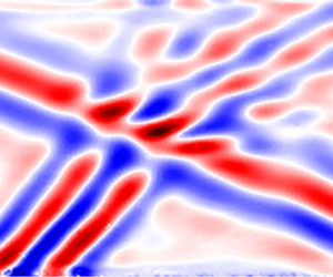
For $\left | \omega \right | < N$ $\left ( \varGamma \in \mathbb {I}, \gamma \in \mathbb {R} \right )$, we obtain propagating solutions with characteristics of gradient $\pm 1 / \gamma$. The imaginary part of the Green's function for $\omega = 0.5N$ is plotted in figure 3. The real part is piecewise constant with discontinuities across the characteristics. When $\left | x - x_0 \right | > \gamma \left | z - z_0 \right |$, the real part equals $1 / ( 4 \omega ^{2} \gamma )$ and equals zero elsewhere. We see a St. Andrew's cross pattern analogous to that produced by a small cylinder undergoing vertical oscillations (Görtler Reference Görtler1943; Mowbray & Rarity Reference Mowbray and Rarity1967). The potential and derived velocities grow unboundedly on approaching the characteristics, which is a consequence of the idealisations (e.g. neglecting viscosity) embedded in this model. Nonetheless, when integrated over point sources of zero area, a finite contribution is obtained in the same way that an integration over $\delta$-functions produces a finite integral, a property we will exploit in § 3.2.

Figure 3. Imaginary component of the propagating Green's function for $\omega = 0.5N$, which shows (a) the streamlines and (b) contours of the internal potential, and the derived velocity fields at time $t = {\rm \pi}/ \left ( 2 \omega \right )$. The velocity indicators have the same scale as those in the evanescent case (figure 2). The potentials and corresponding fluid speeds grow unboundedly at the characteristics, with the largest ones, which would only be visible near the origin, omitted for clarity. The real part is zero in the regions above both characteristics and below both characteristics, and is $1 / ( 4 \omega ^{2} \gamma )$ in the remaining regions to the left of both characteristics and to the right of both characteristics.

For $\left | \omega \right | < N$ $\left ( \gamma \in \mathbb {R} \right )$, the separable form of $r^{2}$ allows us to decompose the argument of the logarithm into two characteristic coordinates,

(3.8)\begin{equation} \eta_{{\pm}} = \left( \frac{x - x_0}{\gamma} \right) \mp \left( z - z_0 \right), \end{equation}

such that the $\eta _+$ characteristics have positive slope and $\eta _-$ negative. The argument of the logarithm, $\left | r^{2} \right |$, becomes a difference of squares because $\varGamma ^{2} < 0$, so decomposes into the characteristic coordinates,

(3.9)\begin{equation} \left| r^{2} \right| = \left| \left[ \left( \frac{x - x_0}{\gamma} \right) - \left( z - z_0 \right) \right] \left[ \left( \frac{x - x_0}{\gamma} \right) + \left( z - z_0 \right) \right] \right| = \left| \eta_+ \eta_- \right| . \end{equation}

Therefore, the logarithm splits into two linearly superposed components with no cross-term,

(3.10)\begin{equation} \log{ \left| r^{2} \right|} = \log{\left| \eta_+ \right|} + \log{ \left| \eta_- \right|} . \end{equation}

The solution to a cylinder undergoing small vertical oscillations shares this decoupling into $\eta _{\pm }$ components (Hurley Reference Hurley1997). In the critical limit $\omega \to N$ from below, the characteristics are vertical, which smoothly transition to the ellipses of contours with infinite aspect ratio in the limit $\omega \to N$ from above.

3.2. Numerical implementation

In general, we are unable to analytically integrate the Green's function, $G_{\omega }$, over the distribution of point sources to determine $\chi _{\omega }$ from (3.2). Consequently, we now seek to use our Green's function solution as the basis for a semi-analytical method to evaluate the potential, $\chi _{\omega }$, at arbitrary locations in space. We anticipate distributed sources, so the potential strength at any evaluation point in space will be composed of a linear superposition of solutions from all sources. Unfortunately, our solution has logarithmic singularities along the characteristics, and so any numerical method based on pointwise evaluation will suffer from unresolvable infinities. However, with careful treatment we may regularise these over finite integration elements, and thus we discretise the domain into elements, $\mathcal {E}\left (\boldsymbol {x}_D \right )$, of size ${\rm \Delta} x \Delta z$. We account for the effect of integrating over an element by introducing a corresponding modified discrete Green's function, $G_D \left ( \boldsymbol {x} ; \boldsymbol {x}_D \right )$, and source distribution, $f_D \left ( \boldsymbol {x}_D \right )$, where the centres of such elements are at $\boldsymbol {x}_D$, so that

(3.11)\begin{equation} \chi_{\omega} \left( \boldsymbol{x} \right) = \sum_{\boldsymbol{x}_D} {G_D \left( \boldsymbol{x}; \boldsymbol{x}_D \right) f_{D} \left( \boldsymbol{x}_D \right)} . \end{equation}

While much of what follows is required to determine $G_D$, we may simply take $f_D \left ( \boldsymbol {x}_D \right ) = \left ( 1 / \left ( \Delta x \Delta z \right ) \right ) \iint _{ {}{\mathcal {E}\left (\boldsymbol {x}_D \right )}} f_{\omega } \left ( \boldsymbol {x}_0 \right ) \, \mathrm {d}^{2} \boldsymbol {x}_0$, integrated over the element. For smooth source distributions, we make the approximation $f_D \left ( \boldsymbol {x}_D \right ) \approx f_{\omega } \left ( \boldsymbol {x}_D \right )$. If instead there is an isolated $\delta$-function source of strength $q$ that lies somewhere within the element, the mean source density is $f_D = q / ( \Delta x \Delta z )$. Correspondingly, a smooth line source distribution of the form $f_{\omega } = q \left ( x \right ) \delta \left ( z - z_0 \right )$ has mean density $f_D \approx q \left ( x_D \right ) / \Delta z$.

We note in passing that while the transformed coordinate system $\left ( \eta _+ , \eta _- \right )$ aligns with the characteristic directions of propagating waves for some $\left | \omega \right | < N$, no single coordinate system would be optimal for a polychromatic wave field (as will be highlighted in § 4). Thus, we opt to discretise a regular Cartesian grid in $\left ( x , z \right )$.

The Green's function only depends on the displacement from the source to the evaluation point, so by moving the reference frame to the centre of the finite element enclosing the source, $\boldsymbol {x}_D$, we may define a continuous variable $\boldsymbol {x}' = \boldsymbol {x} - \boldsymbol {x}_D$ over which we may integrate to determine $G_D$ for all elements. Since the grid is regular, then by accepting a small discretisation error no larger than $\Delta x / 2$, between the location of the source and the centre of the element we only need to calculate the Green's function once for each relative displacement at any given frequency. Then, we translate the resulting array of values according to $\boldsymbol {x}_D$ when evaluating the summation for $\chi _{\omega }$ (3.11), truncating any values that fall outside the numerical domain.

We choose approximate formulae for each evaluation of the Green's function, $G_D$, according to the classification in figure 4. The figure only shows elements in the first quadrant, with the other quadrants deduced by symmetry. In the remainder of this section, we explain the decision points and formulae referenced in the figure.

Figure 4. Classification of finite element types in the first quadrant showing the breakdown according to whether $G_{\omega }$ remains finite within the element, whether propagating or evanescent and by the geometry of the intersections between characteristics and the element boundary. The thumbnail images show $\mbox {Re}{\left \{ G_{\omega } \right \} }$, which equals $1 / ( 4 \omega ^{2} \gamma )$ in the shaded regions and zero elsewhere. Formulae for evaluating $G_D$ are given for each case, and the areas for calculating $\mbox {Re}{\left \{ G_D \right \} }$ in the propagating case are referenced by their case numbers in table 1.

Except at the source and elsewhere near its characteristics, the continuous Green's function is regular and may be approximated by a Riemann sum of the form

(3.12)\begin{equation} G_D \left( \boldsymbol{x} ; \boldsymbol{x}_D \right) \approx G_{\omega} \left( \boldsymbol{x} ; \boldsymbol{x}_D \right) \Delta x \Delta z . \end{equation}

For $\left | \omega \right | > N$, the only singular element is that which encloses $\boldsymbol {x} = \boldsymbol {x}_0$, and in this case the integral is given by

(3.13)\begin{equation} G_D \left( \boldsymbol{x}_D ; \boldsymbol{x}_D \right) = \int_{- \Delta x / 2}^{\Delta x / 2} {\int_{- \Delta z / 2}^{\Delta z / 2} {-\frac{\log{\left( \left( \dfrac{x'}{\varGamma} \right)^{2} + z'^{2} \right)}}{4 {\rm \pi}\omega^{2} \varGamma} \, \mathrm{d} z'} \, \mathrm{d}\kern0.7pt x'} . \end{equation}

The dominant contribution to the integral comes from the logarithm close to the singularity, so we approximate the integral on the rectangular element by an ellipse of equivalent area. After dilatation, the radius, $R$, of the resulting circle is given by ${\rm \pi} R^{2} = \Delta x \Delta z / \varGamma$. We re-express the Green's function in polar coordinates,

(3.14)\begin{equation} G_D \left( \boldsymbol{x}_D ; \boldsymbol{x}_D \right) \approx \int_0^{2 {\rm \pi}} \int_0^{R} {- \frac{\log{\left( r^{2} \right)}}{4 {\rm \pi}\omega^{2} \varGamma} r \, \mathrm{d} r \, \mathrm{d} \theta}. \end{equation}

Integration by parts gives

(3.15)\begin{equation} G_D \left( \boldsymbol{x}_D ; \boldsymbol{x}_D \right) \approx \frac{\Delta x \Delta z}{4 {\rm \pi}\omega^{2} \varGamma^{2}} \left( 1 - \log{\frac{\Delta x \Delta z}{{\rm \pi} \varGamma}} \right). \end{equation}

For the case where internal waves may be generated, $\left | \omega \right | < N$, the imaginary part of the Green's function decomposes into the sum of two linearly independent components (3.10), one for each characteristic direction. Using symmetry, singular elements along the $x'$ or $z'$ axes intersect both characteristics (the case of two characteristics in figure 4). Conversely, singular elements away from the axes may only intersect one characteristic. We calculate each $\eta _{\pm }$ component of $G_D$ separately and then add them together. For elements significantly away from the corresponding characteristic, $\eta _{\pm } = 0$, the component of the Green's function varies approximately linearly across the element and we invoke the centre-value approximation for a regular point (3.12). Otherwise, when the characteristic passes through an element or close to one of its corners, we approximate this component of $G_D$ using integrals as follows.

Let us consider the $\eta _+$ component for a singular element, and define $\eta _R$ and $\eta _L$ to be the maximum and minimum values respectively of $\eta _+ = x' / \gamma - z'$ in this element. Because the level sets of $\eta _+$ are lines of positive gradient and $\eta _+$ is increasing in $x'$, the maximum value of $\eta _+$ occurs in the bottom-right corner of the element and the minimum in the top-left corner, so

(3.16a)\begin{gather} \eta_R = \eta_+ \left( x' + \frac{\Delta x}{2} , z' - \frac{\Delta z}{2} \right) = \frac{x' + \dfrac{\Delta x}{2}}{\gamma} - \left( z' - \frac{\Delta z}{2} \right) , \end{gather}

(3.16b)\begin{gather}\eta_L = \eta_+ \left( x' - \frac{\Delta x}{2} , z' + \frac{\Delta z}{2} \right) = \frac{x' - \dfrac{\Delta x}{2}}{\gamma} - \left( z' + \frac{\Delta z}{2} \right) . \end{gather}

We approximate the contribution across the element by integrating over a rectangle aligned with the characteristic that intersects the element corners where $\eta _+ = \eta _R$ and $\eta _+ = \eta _L$, and then scale the value by the ratio of areas. The contribution to $G_D$ is approximately

(3.17)\begin{align} & \left( \frac{\Delta x \Delta z}{\left| \eta_R - \eta_L \right|} \right) \left( \frac{\mathrm{i}}{4 {\rm \pi}\omega^{2} \gamma} \int_{\eta_L}^{\eta_R} {\log{ \left| \eta_+ \right|} \, \mathrm{d} \eta_+} \right) \nonumber\\ &\quad = \left( \frac{\Delta x \Delta z}{\left| \eta_R - \eta_L \right|} \right) \left( \frac{\mathrm{i}}{4 {\rm \pi}\omega^{2} \gamma} \right) \left( \eta_R \left( \log{\left| \eta_R \right|} - 1 \right) - \eta_L \left( \log{\left| \eta_L \right|} - 1 \right) \right), \end{align}

after integration by parts, where we clarify that $\eta \log {\eta } = 0$ when $\eta = 0$. By symmetry, the same expression holds for the singular contribution due to $\eta _-$ terms.

This leaves the real part of $G_{\omega }$ to consider. It is only non-zero in the regions to the left and to the right of the source bounded by the characteristics, which are shown for the first quadrant as shaded regions in figure 4. The real part of the integral over the element is given by $1 / ( 4 \omega ^{2} \gamma )$ multiplied by the shaded area. We present in table 1 the formulae for all permutations of shaded area expressed in the $\boldsymbol {x}'$ coordinate system centred on an element.

Table 1. Shaded area of each type of singular element centred on $\boldsymbol {x}'$. These thumbnails are shown for quadrant $1$; other quadrants are deduced by symmetry. It is helpful to observe that $\left | x' \right | = \gamma \left | z' \right |$ on the characteristics. In cases 7–10, in addition to the given criteria, we explicitly require that a characteristic passes through the element: in the first and third quadrants, only the $\eta _+$ characteristic may intersect the element, but in the second and fourth quadrants, only the $\eta _-$ characteristic may intersect it. These areas are multiplied by $1 / ( 4 \omega ^{2} \gamma )$ to give $\mbox {Re}{\left \{ G_D \right \} }$.

4.1. Introduction

Internal waves are frequently generated by moving boundaries. For example, in the laboratory, McEwan (Reference McEwan1971, Reference McEwan1973) used articulated paddles and Gostiaux et al. (Reference Gostiaux, Didelle, Mercier and Dauxois2007) used rotating cams, but these are best suited to monochromatic excitations. We installed a ‘magic carpet’ (Dobra et al. Reference Dobra, Lawrie and Dalziel2019) in the base of our tank, which has more general possibilities for excitation. Likewise, we generalise our numerical method for a single frequency, $\chi _{\omega } \exp {\left ( - \mathrm {i} \omega t \right )}$, described in § 3 to those that have a continuous spectrum of frequencies.

For a distribution of sources $f \left ( x , z , t \right ) = \int f_{\omega } \left ( x, z \right ) \exp {\left ( - \mathrm {i} \omega t \right )} \, \mathrm {d} \omega$, we may write

(4.1)\begin{equation} \chi \left( \boldsymbol{x} , t \right) = \int_{\mathbb{R}} {\exp{\left( - \mathrm{i} \omega t \right)} \iint_{\mathbb{R}^{2}} {G_{\omega} \left( \boldsymbol{x}; \boldsymbol{x}_0 \right) f_{\omega} \left( \boldsymbol{x}_0 \right) \mathrm{d}^{2} \boldsymbol{x}_0}} \, \mathrm{d} \omega. \end{equation}

Our numerical method allows replacement of these integrals with the discrete Fourier transform, and thus we may approximate general wave fields. We summarise our procedure in algorithm 1. In the special case of a discrete set of input frequencies, we no longer need to resolve the Fourier transform and all the frequencies can be represented exactly.

Algorithm 1 Calculation of potential χ for an arbitrary source distribution f(x, t). It is calculated mode by mode using the discrete monochromatic Green's function, G _D. At each frequency, we first evaluate f _D and G _D, then finally we accumulate contributions to the potential field.

In our model, we consider flexible boundaries as sources of either volume or vorticity. As we saw in § 2, source terms in the internal wave equation for internal potential and streamfunction represent volume and vorticity sources respectively. We now derive formulae for the source terms of both potentials, $\xi$ and $\psi$, to describe each temporal mode of an arbitrary vertical displacement of a horizontal boundary.

4.2. Representing active boundaries with finite element sources

In both cases, we can readily derive volume fluxes for a monochromatic source of unit strength by integrating the Green's function, so we rescale these fluxes to match a discrete physical representation of a short distance along the boundary. The rescaling factors are collectively the required distribution of sources along the entire length of the boundary. Here, we outline the method and summarise key results; see §§ 4.2.1 and 4.2.2 for full derivations. Throughout this section, all sources are at the zero-height of the magic carpet, so without loss of generality we take $z_0 = 0$.

We seek to determine the volume flux, $Q \left ( t \right ) = Q_{\omega } \exp {\left ( - \mathrm {i} \omega t \right )}$, induced by a monochromatic source of unit strength across a transect of the domain. For the internal potential, the transect is a horizontal line at $z > 0$ ranging from $x = -\infty$ to $+ \infty$, across which the flux amplitude $Q_{\omega } = \frac {1}{2}$. Whereas, the corresponding transect for the streamfunction is a vertical line segment to the right of the wave maker (assuming the case of rightward propagating waves, $\omega k >0$) ranging from $z = 0$ to $+ \infty$, across which $Q_{\omega } = 1 / ( 4 \omega ^{2} \gamma )$. In both cases, we find that the component of the Green's function flow satisfying the conditions imposed by the physical model of the magic carpet is in phase with the forcing, $\mbox {Re}{\left \{ Q_{\omega } \right \} }$, and the implied flow has the form of linear jets along the characteristics, which can be represented by $\delta$-functions.

The total volume flux from one finite grid element of width $\Delta x$ and height $\Delta z$ that is centred on $\left ( x_D , 0 \right )$ and contains the distribution of monochromatic point sources $f = f_{\omega } \left ( x , z \right ) \exp {\left ( - \mathrm {i} \omega t \right )}$ is

(4.2)\begin{align} \int_{x_D - \Delta x / 2}^{x_D + \Delta x / 2}{\int_{- \Delta z / 2}^{\Delta z / 2}{Q_{\omega} f_{\omega} \left( x', z' \right) \exp{\left( - \mathrm{i} \omega t \right)} \, \mathrm{d} z'} \, \mathrm{d}\kern0.7pt x'} \approx \Delta x \Delta z Q_{\omega} f_{\omega} \left( x_D , 0 \right) \exp{\left( - \mathrm{i} \omega t \right)} . \end{align}

Then, we equate this expression with the corresponding volume flux, $R \left ( t \right ) = R_{\omega } \exp {\left ( - \mathrm {i} \omega t \right )}$, predicted by a physical model of volume displacement by the wave maker surface to obtain the distribution of sources,

(4.3)\begin{equation} f_{\omega} \left( x_D , 0 \right) = \frac{R_{\omega}}{\Delta x \Delta z Q_{\omega}} . \end{equation}

For the internal potential, $R_{\omega } = - \mathrm {i} \omega \Delta x h_{\omega } \left ( x_D \right )$, so

(4.4a)\begin{equation} f_{\omega} \left( x_D , 0 \right) ={-} \frac{2 \mathrm{i} \omega}{\Delta z} h_{\omega} \left( x_D \right) . \end{equation}

Whereas, for the streamfunction, $R_{\omega } = - ( \mathrm {i} \omega \Delta x / 2 ) h_{\omega } \left ( x_D \right )$, so

(4.4b)\begin{equation} f_{\omega} \left( x_D , 0 \right) ={-} \frac{2 \mathrm{i} \omega^{3} \gamma}{\Delta z} h_{\omega} \left( x_D \right) . \end{equation}

4.2.1. Internal potential

For the internal potential, we determine the total vertical volume flux through a line of constant $z \neq 0$,

(4.5)\begin{equation} Q \left( z , t \right) = Q_{\omega} \left( z \right) \exp{\left( - \mathrm{i} \omega t \right)} = \int_{-\infty}^{\infty} w \left( x, z , t \right) \,\mathrm{d}\kern0.7pt x, \end{equation}

for the Green's function when $0 < \omega < N$. The vertical velocity field, $w$, is given by $\partial ^{3} \left ( G_{\omega } \exp {\left ( - \mathrm {i} \omega t \right )} \right ) / \partial t^{2} \partial z$ and thus $w = - \omega ^{2} ( \partial G_{\omega } / \partial z ) \exp {\left ( - \mathrm {i} \omega t \right )}$. Since the following is equally applicable to continuous and discretised sources, we adopt $\left (x_0,z_0\right )$ notation to represent a source. Applying the chain rule to $G_{\omega }$ (3.7) when $z_0 = 0$, we obtain

(4.6)\begin{equation} \frac{\partial G_{\omega}}{\partial z} ={-} \mathrm{i} \frac{z}{2 {\rm \pi}\omega^{2} \gamma \left[ \left( \dfrac{x - x_0}{\gamma} \right)^{2} - z^{2} \right]} - \frac{z}{2 \omega^{2} \gamma} \delta{\left( \left( \frac{x - x_0}{\gamma} \right)^{2} - z^{2} \right)}. \end{equation}

Along a path of constant $z$ (where $z \neq 0$) as shown in figure 5, the imaginary part has two simple poles, $x = x_0 \pm \gamma z$, which are where the path crosses the characteristics of $G_{\omega }$, and $\partial G_{\omega } / \partial z$ asymptotes inverse–linearly towards them. Between the poles (in the line segment containing $x = x_0$), ${{\rm sgn}}{\left ( \mbox {Im}{\left \{ \partial G_{\omega } / \partial z \right \}} \right )} = + {{\rm sgn}}{\left ( z \right )}$, and outside the poles (where $x \to \pm \infty$), ${{\rm sgn}}{\left ( \mbox {Im}{\left \{ \partial G_{\omega } / \partial z \right \} } \right )} = - {{\rm sgn}}{\left ( z \right )}$. Thus, we may use the Cauchy principle value to regularise $Q_{\omega }$ at each pole. The imaginary part exhibits even symmetry about $x = x_0$, so it suffices to consider only half of the domain and double the result,

(4.7)\begin{align} \mbox{Im}{\left\{ Q_{\omega} \left( z \right) \right\}} = \lim_{\epsilon \to 0} \left\{ \frac{z}{{\rm \pi} \gamma} \left( \int_{x_0}^{x_0 + \gamma z - \epsilon} \frac{\mathrm{d}\kern0.7pt x}{\left( \dfrac{x - x_0}{\gamma} \right)^{2} - z^{2}} - \int_{x_0 + \gamma z + \epsilon}^{\infty} \frac{\mathrm{d}\kern0.7pt x}{\left( \dfrac{x - x_0}{\gamma} \right)^{2} - z^{2}} \right) \right\} . \end{align}

Factoring out $z^{2}$ and using the substitution $p = \left ( x - x_0 \right ) / \left ( \gamma z \right )$ leaves

(4.8)\begin{equation} \mbox{Im}{\left\{ Q_{\omega} \left( z \right) \right\}} = \lim_{\epsilon \to 0} \left\{ \frac{1}{\rm \pi} \left( \int_{0}^{1 - \epsilon / ( \gamma z )}{\frac{\mathrm{d} p}{p^{2} - 1}} - \int_{1 + \epsilon / ( \gamma z )}^{\infty}{\frac{\mathrm{d} p}{p^{2} - 1}} \right) \right\} . \end{equation}

The scaling on the limit variable, $\epsilon$, is the same for both integrals, so we may replace the corresponding limits on the integrals by $1 \mp \epsilon$. Then, evaluating the definite integrals yields

(4.9)\begin{equation} \mbox{Im}{\left\{ Q_{\omega} \left( z \right) \right\}} = \lim_{\epsilon \to 0} {\left\{ \frac{1}{2 {\rm \pi}} \left( \left[ \log{\frac{1 - p}{1 + p}} \right]_0^{1-\epsilon} - \left[ \log{\frac{p - 1}{p + 1}} \right]_{1+\epsilon}^{\infty} \right) \right\}} = 0 . \end{equation}

Figure 5. Integration path for calculating the volume flux, $Q$, for the internal potential, showing the locations of the poles in the imaginary part of $\partial G_{\omega } / \partial z$, which are also the locations of the singularities in the real part.

Next, we consider the integral over the $\delta$-function in the real part. Along a path of constant $z$, the argument of the $\delta$-function has two simple zeros, $y_{1,2} = x_0 \pm \gamma z$, for which we use the standard formula,

(4.10)\begin{equation} \delta \left( f \left( x \right) \right) = \sum_{k = 1}^{2} \frac{\delta \left( x - y_k \right)}{\left| \left. \dfrac{\mathrm{d} f}{\mathrm{d}\kern0.7pt x} \right|_{y_k} \right|}. \end{equation}

Here, $\mathrm {d} f / \mathrm {d} x = 2 ( x - x_0 ) / \gamma ^{2}$, so we have

(4.11)\begin{equation} \mbox{Re}{\left\{ Q_{\omega} \left( z \right) \right\}} = \int_{- \infty}^{\infty}{\frac{z}{2 \gamma} \left( \frac{\delta \left( x - \left[ x_0 + \gamma z \right] \right)}{\left| \dfrac{2}{\gamma^{2}} \gamma z \right|} + \frac{\delta \left( x - \left[ x_0 - \gamma z \right] \right)}{\left| - \dfrac{2}{\gamma^{2}} \gamma z \right|} \right) \, \mathrm{d}\kern0.7pt x}. \end{equation}

Each $\delta$-function contributes a value of one to the integral and $z / | z | = {{\rm sgn}}{\left ( z \right )}$, so $\mbox {Re}{\{ Q_{\omega } \left ( z \right ) \}} = \frac {1}{2} {{\rm sgn}}{\left ( z \right )}$. Therefore, $Q \left ( z \right ) = \frac {1}{2} {{\rm sgn}}{\left ( z \right )} \exp {(-\mathrm {i} \omega t)}$.

The total vertical volume flux through a horizontal transect is half the strength of the internal potential point source and is in phase with the source. The flux has a vertical component everywhere except $z = 0$ and points away from the source when the source is positive. Closing a rectangular contour along $z = \pm z_0$ and $x = \pm \infty$, symmetry arguments determine that the vertical integrals at $x = \pm \infty$ are both zero and integration along the horizontal edges doubles due to the direction in which they are taken. Thus, a monochromatic point source of internal potential of unit strength forces the internal wave equation such that the total volume flux is monochromatic and of unit strength.

We remark that this result also applies to a corresponding integral when the Green's function is for the streamfunction,

(4.12)\begin{equation} \int_{-\infty}^{\infty}{-u \, \mathrm{d}\kern0.7pt x} = \int_{-\infty}^{\infty}{\frac{\partial G_{\omega}}{\partial z} \, \mathrm{d}\kern0.7pt x} = \frac{1}{2} {{\rm sgn}}{\left( z \right)} \exp{\left( -\mathrm{i} \omega t \right)} . \end{equation}

Using the same rectangular contour, we obtain the circulation around the point source to be $\frac {1}{2} \exp {(-\mathrm {i} \omega t)}$. Letting $z \to 0$ so that the area enclosed in the contour tends to zero and invoking Stokes’ theorem shows that the source is a point vortex of strength $\frac {1}{2} \exp {(-\mathrm {i} \omega t)}$.

Similar to a resonant simple harmonic oscillator, there are components of the internal potential field both in phase to the forcing and with a phase lag of a quarter oscillation behind the source. Here, the in-phase response ensures the conservation of volume by generating line jets only and exactly along the characteristics, while the phase-lagged response has zero net volume flux despite inducing a flow over the whole domain.

Physically modelling the wave maker, the upwards volume flux generated by an element with vertical displacement $h$, as shown in figure 6, is

(4.13)\begin{equation} R \left( t \right) = \int_{x_D - \Delta x / 2}^{x_D + \Delta x / 2}{\frac{\partial h}{\partial t} \, \mathrm{d}\kern0.7pt x'}, \end{equation}

which is approximately equal to $- \mathrm {i} \omega \, \Delta x \, h_{\omega } \exp {(-\mathrm {i} \omega t)}$ for small elements. Substituting this into the formula for the required element source strength (4.3) yields the required source strengths for use in the discrete Green's function, $f_{\omega } \left ( x_D , 0 \right ) = - ( 2 \mathrm {i} \omega / \Delta z ) h_{\omega } \left ( x_D \right )$.

Figure 6. Finite element of width $\Delta x$ representing wave maker displacement at a single location. We use this model to calculate the induced vertical volume flux required for sources to the internal potential, which is $\Delta x \left. \partial h / \partial t \right |_{\left ( x_D , t \right )}$. The vertical dashed lines indicate the element centrelines.

4.2.2. Streamfunction

When the Green's function represents the streamfunction, the volume flux across any horizontal or vertical transect is zero, because sources in the streamfunction internal wave equation are vortices. Instead, since the volume flux across a path is equal to the difference between the values of the streamfunction at each end, we note that the real part of the volume flux induced by $G_{\omega }$ (3.7) across any semi-infinite vertical line from $z = 0$ to $z = \infty$ for constant $x$ is $Q_{\omega } = 1 / ( 4 \omega ^{2} \gamma )$. The point vortex is in phase with the source, so it is not necessary to consider the imaginary part.

For the physical model, we consider a wave maker profile that is spatially sampled every $\delta x$ and is zero everywhere except at one sample point, $x = x_p$, as shown in figure 7. We assume that the wave maker is piecewise linear between the sample points. The rightwards volume flux generated to the right of the displaced infinitesimal element is $R \left ( x_p + \delta x , t \right ) = ( \Delta x / 2 ) \partial h / \partial t |_{\left ( x_p , t \right )}$. Conversely, the rightwards volume flux to the left of the element is $R \left ( x_p - \delta x , t \right ) = - ( \Delta x / 2 ) \partial h / \partial t |_{\left ( x_p , t \right )}$. In the continuum limit, we have

(4.14)\begin{equation} \left. \frac{\partial R}{\partial x} \right|_{\left( x_p , t \right)} = \lim_{\delta x \to 0}{\frac{R \left( x_p + \delta x , t \right) - R \left( x_p - \delta x , t \right)}{2 \delta x}} = \frac{1}{2} \left. \frac{\partial h}{\partial t} \right|_{\left( x_p , t \right)}. \end{equation}

Integrating such point contributions over a finite element of width $\Delta x$ centred on $\left ( x_D , 0 \right )$ gives the total horizontal volume flux across one source element,

(4.15)\begin{equation} R \left( x_D , t \right) = \int_{x_D - \Delta x / 2}^{x_D + \Delta x / 2}{\frac{1}{2} \frac{\partial h}{\partial t} \, \mathrm{d}\kern0.7pt x} \approx \frac{\Delta x}{2} \left. \frac{\partial h}{\partial t} \right|_{\left( x_D , t \right)} , \end{equation}

to leading order in $\Delta x$. Thus, $R_{\omega } = - ( \mathrm {i} \omega \Delta x / 2 ) h_{\omega } \left ( x_D \right )$ and

(4.16)\begin{equation} f_{\omega} \left( x_D , 0 \right) ={-} \frac{2 \mathrm{i} \omega^{3} \gamma}{\Delta z} h_{\omega} \left( x_D \right) . \end{equation}

Figure 7. Infinitesimal element representing wave maker displacement at a single location, assuming the profile to be linear between sample points $\delta x$ apart and the domain to have a rigid lid. We use this model to calculate along-wave maker gradients of induced horizontal volume flux, whose integrals are required for finite sources of width $\Delta x$ to the streamfunction.

4.3. Boundary considerations

Non-zero-frequency internal waves in a finite domain will inevitably reflect off the top and bottom. In both cases, the fluid cannot flow across the boundary, so we take $w = 0$ as the boundary condition and exploit the characteristic structure of internal waves to enforce it. The required potential, $\chi$, for the reflected wave is calculated along the boundary and then projected along its characteristics using an approach introduced in Dobra et al. (Reference Dobra, Lawrie and Dalziel2021). The characteristics of the reflected wave are oriented in the opposite vertical, but same horizontal, direction as the incident wave.

For the internal potential in a monochromatic flow, $w = - \omega ^{2}\partial \xi / \partial z$ and on the boundary, the reflected wave may take the same value of the internal potential as the incident wave. By contrast, the vertical velocity is obtained from the streamfunction as $w = \partial \psi / \partial x$, giving $\psi = \textrm {const.}$ on the boundary, so we require that the reflected streamfunction is the negative of the incident. In both cases, we set the gauge constant to zero for convenience.

Evaluating $\chi$ only on the boundary is insufficient to deduce the horizontal direction of incident characteristics. A wave field of a particular frequency may contain waves in all directions, so we use a principal axes transformation to decompose the incident wave field into left- and right-travelling waves according to the direction of the gradient vector (Dobra Reference Dobra2018, pp. 37–39) and reflect each component in turn.

The interference pattern arising from the distribution of sources generates the desired wave field, but where the source array is abruptly truncated, powerful harmonics are emitted and they may contaminate the solution within the domain. To reduce the severity of such truncation, we smoothly reduce the source strength to zero at the lateral extremities of the calculation domain according to a $C^{3}$-continuous ramp that extends well beyond the field of view. Similarly, we use a significantly extended temporal domain for the Fourier transform to avoid periodic reflection in time activity that is aperiodic and short in duration.

4.4. Experimental method

The ‘magic carpet’ or Arbitrary Spectrum Wave Maker (Dobra et al. Reference Dobra, Lawrie and Dalziel2019) is a flexible 1 m long and flush with the base of a tank that is 11 m long, 0.255 m wide and 0.48 m deep. The magic carpet's shape is controlled by an array of $100$ linear stepper motors positioned at a pitch of 10 mm, each with a vertical resolution of 0.0127 mm and a stroke of 48 mm.

The surface of the wave maker is a nylon-faced neoprene foam sheet of thickness 3 mm. The material has some resistance to bending, but the attachment mechanism is designed to minimise the tensile stress in the sheet and the bending moments on the actuating rods. We model the surface deformations at each instant, $h \left ( x , t \right )$, as satisfying

(4.17)\begin{equation} \frac{Es^{3}}{12} \frac{\partial^{4} h}{\partial x^{4}} - T \frac{\partial^{2} h}{\partial x^{2}} = p_* , \end{equation}

where $E$ is Young's modulus, $s$ is the sheet thickness, $T$ is the longitudinal tension in the sheet and $p_*$ is the pressure difference across the sheet, normally taken as zero. Defining $\lambda = ( 12 T / ( E s^{3} ) )^{1/2}$, this equation has eigensolutions $\boldsymbol {f} \left ( x \right ) = \left [\begin {smallmatrix} 1 & x & \cosh {\lambda x} & \sinh {\lambda x}\end {smallmatrix}\right ]^{\operatorname {T}}$. For our magic carpet, we find that $\lambda \approx 400$. These solutions differ from the typical Euler–Bernoulli linear beam by the presence of hyperbolic functions instead of cubic polynomials, and these differences arise from longitudinal tension. Defining a vector of constants $\boldsymbol {b}$ to be determined by the rod heights and enforcing $C^{2}$-continuity, the general solution between each rod is $h \left ( x \right ) = \boldsymbol {b} \boldsymbol {\cdot } \boldsymbol {f} \left ( x \right )$. Combining the boundary conditions for all sections of the wave maker gives a linear system of equations with constant coefficients, which can be easily inverted numerically.

We fill the tank using the double bucket method (Fortuin Reference Fortuin1960; Oster Reference Oster1965) with a linear density stratification in brine producing a constant buoyancy frequency $N = 1.45\,{\rm rad}\,{\rm s}^{-1}$. We observe density perturbations using Synthetic Schlieren, an optical technique (Dalziel et al. Reference Dalziel, Hughes and Sutherland1998; Sutherland et al. Reference Sutherland, Dalziel, Hughes and Linden1999; Dalziel et al. Reference Dalziel, Hughes and Sutherland2000). A static, random pattern of black and white dots is displayed on a 4k (UHD) television screen measuring 1.4 m $\left ( 55'' \right )$ on the diagonal that is 0.2 m behind the tank, following Sveen & Dalziel (Reference Sveen and Dalziel2005). The light rays emitting from the screen bend as they pass through the varying refractive indices in the tank, and the distorted images are recorded at $4\,\textrm {f.p.s.}$ on a 12-megapixel ISVI IC-X12CXP video camera located 3.8 m in front of the tank. A pattern-matching algorithm in the software package DigiFlow (Dalziel Research Partners 2018) is used to reconstruct the gradient of the density perturbation from the recorded images, and we plot its horizontal component, which is related to the internal potential according to $( 1 / \rho _{00} ) \partial \rho ' / \partial x = ( N^{2} / g ) \partial ^{3} \xi / \partial x \partial z \partial t$ for linear waves.

4.5. An example: atmospheric lee waves

A travelling solitary hump is perhaps the simplest aperiodic waveform, directly analogous to flow over an isolated mountain ridge (Dalziel et al. Reference Dalziel, Patterson, Caulfield and Le Brun2011). In our experiments, the fluid is stationary in the tank, so boundary layers do not form upstream and we obtain cleaner waveforms.

We seek to validate our numerical model in this configuration, and we choose to calculate the wave field using the internal potential, although we could equally obtain the same wave field using the streamfunction. Our hump consists of a complete wavelength of a sinusoid ranging from trough to trough, where the troughs are flush with the zero height of the magic carpet, with wavelength 0.081 m and peak-to-trough amplitude 0.028 m propagating to the right at $U = 0.0357\,{\rm m}\,{\rm s}^{-1}$. We use $1024$ points spanning 50 s for the discrete Fourier transform, giving a frequency resolution of 0.13 rad s$^{-1}$. The hump takes 2.3 s to pass any fixed location, which corresponds to a frequency of 2.8 rad s$^{-1}$. With this adequate temporal resolution, we thus avoid spurious reflections in the time domain.

The passing time of the hump corresponds to a frequency ratio of $\omega / N = 1.88$, which is evanescent. Thus, it is clear that in this case the propagating modes will arise only from peripheral harmonics in the spectrum, an observation to which we will return in § 5. Figure 8 compares our experiments with the wave train predicted by our model.

Figure 8. Prediction and experiment comparing $( 1 / \rho _{00} ) \partial \rho ' / \partial x$ for a solitary sinusoidal hump of height 0.028 m and width 0.081 m moving at $U = 0.0357\,{\rm m}\,{\rm s}^{-1}$. Each image is separated by 5 s, and $N = 1.45\,{\rm rad}\,{\rm s}^{-1}$. The majority of the wave energy exists in waves phase-locked with the hump, and these waves are restricted to a semi-circular envelope, indicated by the black arc. Wave energy to the right of the arc is carried by non-phase-locked waves, but whose spectrum results in a quasi-steady pattern of waves moving with the hump. There are also evanescent modes forming an interference pattern near the hump, but due to discretisation of the temporal spectrum in our prediction, some leakage of energy occurs along the wave maker surface but the response remains localised.

Firstly, from selective withdrawal of modes in our numerical prediction, we deduce that there are significant evanescent modes local to the hump, whose interference pattern is required to capture the structure of the wave train observed in the experiment.

Secondly, we see disturbances spread across the domain, both in front and behind the hump. The waves ahead of the hump appear to be quasi-stationary and persist in the observed timeframe between six and eleven passing periods of the hump after its release. We conclude that these are not simply startup transients, and so we use geometric reasoning to understand the distribution of wave energy in the system.

One common approach is to use the principle of stationary phase (e.g. Lighthill Reference Lighthill1978) to restrict our analysis to elements of the wave field that move in phase with the hump. The solitary hump may be characterised as a broadband spectrum of modes all travelling with a common horizontal phase velocity, $\omega / k = U$. It follows that for a given range of wavenumbers, $k$, there must directly correspond a range of frequencies, $\omega$. Thus, any internal wave propagation generated by the hump has no preferential direction but must share the same horizontal component of phase velocity. The dispersion relation (2.7) constrains the magnitudes of all such wavevectors to the circle $\left | \boldsymbol {k} \right | = N / U$. Consequently, for positive frequencies and upwards propagation, only fourth-quadrant wavevectors remain, and their corresponding group velocities point into the first quadrant. These modes comprise the majority of the observed signal, and their superposition results in curved phase lines. Furthermore, by following rays traced parallel to each mode's respective group velocity, we may determine a propagation envelope for this class of quasi-steady wave. This envelope forms a semi-circle joining the hump's current and initial release locations (Dalziel et al. Reference Dalziel, Patterson, Caulfield and Le Brun2011), as shown by black arcs in figure 8. These advancing semi-circles grow in radius until the envelope asymptotically forms a vertical front.

Clearly, both the experiment and the prediction contain waves propagating ahead of this envelope, so, as previously noted by Voisin (Reference Voisin1994), the principle of stationary phase is insufficient to account for the whole wave field. Given that there is signal high above the wave maker and ahead of the hump, we deduce that these waves must have significant vertical component to their group velocity and therefore have non-zero frequency. Moreover, for internal waves the horizontal component of the group velocity is bounded above by the horizontal component of the phase velocity, and any observable wave ahead of the hump must have group velocity with horizontal component greater than $U$, so the same must also be true for its phase velocity. Although counterintuitive, it is possible for a composition of modes from a spectrum of phase velocities to form a quasi-steady wave field that translates with a single apparent phase velocity. Akin to the decomposition of a standing wave into opposing travelling waves, a carefully chosen difference of frequencies is sufficient to create the required behaviour, although many combinations of wavevector and frequency would also produce an equivalent result. We conjecture that just such a superposition of modes is responsible for propagation ahead of the envelope shown in figure 8.

We note that our approach requires the Fourier transform in time of the entire timeline. Since the source strengths are zero at all times except when the hump is passing, the $\omega$-spectrum is broad. However, a discrete Fourier transform introduces discretisation error, which when inverted produces sources at unwanted times. We see their effect as forced oscillations along the magic carpet, which have insignificant effect on the rest of the wave field.

Our wave propagation model does not directly account for energy leaving the modelled system during a reflection, yet is present in the experiments. We employed a line-search optimisation to determine suitable calibration parameters and accordingly multiply the amplitude of the reflections at the free top surface by $0.6$ while maintaining pure reflections at the solid bottom boundary. Figure 9 demonstrates the necessity of accounting for this energy loss.

Figure 9. Predictions assuming pure reflections (a) and with calibrated attenuation at the free surface with coefficient $0.6$ (b) compared with experiment (c). These correspond to figure 8 at 25 s and show $( 1 / \rho _{00} ) \partial \rho ' / \partial x$. Without attenuation, the predicted amplitude of the wave field behind the hump is larger than observed. The reflection coefficient accounts for energy dissipated at the free surface through mechanisms not directly modelled.

5.1. Introduction

The literature on internal wave laboratory experiments can be divided into two broad lines of enquiry: work following from Görtler (Reference Görtler1943) and Mowbray & Rarity (Reference Mowbray and Rarity1967) on waves generated by a small oscillating body, and work on quasi-monochromatic line sources following McEwan (Reference McEwan1971, Reference McEwan1973). The capability of our magic carpet allows us to span the range between these limiting cases, and although previous work using it (Dobra et al. Reference Dobra, Lawrie and Dalziel2021) validated new theoretical predictions in the line-source limit, we seek here to demonstrate the generality of these findings by applying them to an intermediate regime. We examine the interactions of finite-width wave beams a few wavelengths across, since recent explorations of such configurations (Smith & Crockett Reference Smith and Crockett2014) have uncovered a rich dynamical structure. We have unparalleled access to observe and analyse such wave fields processed first with synthetic Schlieren and then with Dynamic Mode Decomposition (DMD, Schmid Reference Schmid2010). For the cases we consider here, DMD is an ideal tool because the frequency discretisation is responsive to the input, so it takes many fewer samples to accurately recover the dominant frequencies compared with Fourier methods, which project onto basis functions at a fixed discretisation. Furthermore, DMD enables us to distinguish between steady-state behaviours and transient modes. Our experiments have been carefully configured so that steady-state behaviours dominate, and we do not observe the common unsteady phenomenon of triadic resonant instability.

5.2. A series expansion for triadic interactions

Building on the recent developments of Dobra et al. (Reference Dobra, Lawrie and Dalziel2021), here we introduce a fusion of our perturbation expansion framework and the method of solution by Green's function, enabling the construction of general wave fields from the interference patterns produced by a distribution of sources. In Dobra et al., the perturbation expansion at each order yields the internal wave equation in terms of the streamfunction with sources that are Jacobian determinants. Under particular symmetries, we found that these sources cancel, preventing a broad class of wave–wave interactions from occurring. Here, we instead consider configurations where these sources play a significant role in the structure of the wave field, and employing the Green's function with the streamfunction potential, it integrates naturally. We now outline a generalisation of our perturbation framework for these arbitrary wave fields.

We reformulate the conservation of momentum (2.1) and mass (2.3) in terms of streamfunction, $\psi$, and buoyancy, $b = - g \rho ' / \rho _{00}$,

(5.1a)\begin{gather} \frac{\partial}{\partial t} \nabla^{2} \psi + \left| \frac{\partial \left( \psi , \nabla^{2} \psi \right)}{\partial \left( x, z \right)} \right| = \frac{\partial b}{\partial x}, \end{gather}

(5.1b)\begin{gather}\frac{\partial b}{\partial t} + \left| \frac{\partial \left( \psi , b \right)}{\partial \left( x, z \right)} \right| ={-} N^{2} \frac{\partial \psi}{\partial x}, \end{gather}

where the Jacobian determinant of two scalars, $\alpha$ and $\beta$, is given by

(5.2)\begin{equation} \left| \frac{\partial \left( \alpha, \beta \right)}{\partial \left( x, z \right)} \right| = \frac{\partial \alpha}{\partial x} \frac{\partial \beta}{\partial z} - \frac{\partial \alpha}{\partial z} \frac{\partial \beta}{\partial x} . \end{equation}

Eliminating the linear $b$ terms leaves the nonlinear internal wave equation,

(5.3)\begin{equation} \frac{\partial^{2}}{\partial t^{2}} \nabla^{2} \psi + N^{2} \frac{\partial^{2} \psi}{\partial x^{2}} = \frac{\partial}{\partial t} \left| \frac{\partial \left( \nabla^{2} \psi , \psi \right)}{\partial \left( x, z \right)} \right| + \frac{\partial}{\partial x} \left| \frac{\partial \left( b , \psi \right)}{\partial \left( x, z \right)} \right| . \end{equation}

Nonlinearity associated with triadic interactions is captured by source terms of the form of Jacobian determinants, and here we consider their behaviour in the case

(5.4)\begin{equation} \psi = \sum_{j = 1}^{3}{\left\{ A_j \exp{\left( \mathrm{i} \left[ \boldsymbol{k}_j \boldsymbol{\cdot} \boldsymbol{x} - \omega_j t \right] \right)} + A_j^{*} \exp{\left( - \mathrm{i} \left[ \boldsymbol{k}_j \boldsymbol{\cdot} \boldsymbol{x} - \omega_j t \right] \right) } \right\}} , \end{equation}

where we require complex conjugate $\left ( {}^{*} \right )$ pairs to represent real wave fields. The source terms multiply pairs of waves, so we must consider each possible pairing in turn. Self-interactions equate to zero (McEwan Reference McEwan1973; Tabaei & Akylas Reference Tabaei and Akylas2003; Dobra et al. Reference Dobra, Lawrie and Dalziel2021), but the interaction of beam $j = 1$ with beam $j = 2$ produces terms proportional to $\exp {\left ( \mathrm {i} \left [ \left ( \boldsymbol {k}_2 + \boldsymbol {k}_1 \right ) \boldsymbol {\cdot } \boldsymbol {x} - \left ( \omega _2 + \omega _1 \right ) t \right ] \right ) }$, $\exp {\left ( \mathrm {i} \left [ \left ( \boldsymbol {k}_2 - \boldsymbol {k}_1 \right ) \boldsymbol {\cdot } \boldsymbol {x} - \left ( \omega _2 - \omega _1 \right ) t \right ] \right ) }$ and their complex conjugates. Thus, by index manipulation we may define

(5.5a)\begin{gather} \boldsymbol{k}_3 = \boldsymbol{k}_2 \pm \boldsymbol{k}_1 , \end{gather}

(5.5b)\begin{gather}\omega_3 = \omega_2 \pm \omega_1 . \end{gather}

Should this disturbance characterised by $\boldsymbol {k}_3$ and $\omega _3$ satisfy the dispersion relation (2.7), $\omega _3 = N k_3 / \left | \boldsymbol {k}_3 \right |$, the disturbance is also a wave and the source terms are an eigensolution of the internal wave equation (2.9). Such combinations are commonly described as resonant triads.

We examine in figure 10(a) the geometric permutations of wave triad that may be constructed for a given $\boldsymbol {k}_1$, $\omega _1$ and fixed frequency $\omega _2$ but where wavevector $\boldsymbol {k}_2$ is unconstrained. These triangles are compatible with the selection rules derived by Tabaei et al. (Reference Tabaei, Akylas and Lamb2005) and Jiang & Marcus (Reference Jiang and Marcus2009) that determine into which quadrants, if any, a new wave beam may be emitted. These configurations are typical of wave beams a few wavelengths across for which the wavenumber spectra are broad. In these cases, the spectrum of the source terms is significant across a patch of wavevector space, as shown in figure 10(b). Wavevectors that lie on the dashed locus of dispersion-relation-satisfying $\boldsymbol {k}_3$ will resonate, and new waves will emerge by mode selection; these correspond to cases where the triangle of wavevectors can be closed.

Figure 10. Wavevector triangles for the sum of frequencies $\omega _1 + \omega _2$ in the case $\omega _1 = 0.55\,{\rm rad}\,{\rm s}^{-1} = 0.37 N$ and $\omega _2 = 1.5 \omega _1$. In (a), all permutations of wavevector triangles are presented for the case where $\boldsymbol {k}_1$ points into the first quadrant. The triangles for all other quadrants are obtained by reflective symmetry. From the dispersion relation (2.7), each frequency has four possible directions for its wavevector, one in each quadrant. Given $\boldsymbol {k}_1$, the loci of $\boldsymbol {k}_2$ and $\boldsymbol {k}_3$ will in general close to form a triangle in one of four different ways. A closed triangle is a resonant triad. In (b), we plot in greyscale the distribution of source term amplitudes in Fourier space for incident wavevector distributions $\boldsymbol {k}_1$ (blue) and $\boldsymbol {k}_2$ (red). The resonant, propagating $\boldsymbol {k}_3$ lie at the intersections of each of the dashed lines with regions of significant source amplitude. The remainder produce a local interference pattern of forced oscillations. In this configuration, two waves at $\omega _3$ are emitted: a weaker one with $\boldsymbol {k}_3$ pointing into the first quadrant (wave propagating down and to the right, triangle marked in orange in (a)), and a stronger one with $\boldsymbol {k}_3$ pointing into the fourth quadrant (up and to the right, green triangle in (a)).

No polychromatic solutions containing multiple horizontal phase velocities are known for the fully nonlinear equation (5.3), so in Dobra et al. (Reference Dobra, Lawrie and Dalziel2021), we performed a perturbation expansion to give a recursive algorithm that we can truncate at finite order to calculate an approximate solution. In this earlier work, we expanded $\psi$ in powers of a small parameter, $a$, which we took to be the wave steepness. Instead, here we modify the expansion to be $\psi = \sum _{n = 1}^{\infty } \psi _n$, where each subsequent term drops an order of magnitude, and the expansion for $b$ behaves correspondingly. Then, as our earlier work showed, each order satisfies

(5.6)\begin{equation} \frac{\partial^{2}}{\partial t^{2}} \nabla^{2} \psi_n + N^{2} \frac{\partial^{2} \psi_n}{\partial x^{2}} = \sum_{p=1}^{n-1}{\left\{ \frac{\partial}{\partial t} \left| \frac{\partial \left( \nabla^{2} \psi_{p} , \psi_{n-p} \right)}{\partial \left( x, z \right)} \right| + \frac{\partial}{\partial x} \left| \frac{\partial \left( b_{p} , \psi_{n-p} \right)}{\partial \left( x, z \right)} \right| \right\} } . \end{equation}

There is a cascade of information from lower order to higher, but not in reverse, thus the expansion is purely inductive. However, at all orders greater than three, there are contributions to frequencies that already exist at lower orders. There is an infinite series of such contributions to the wave field, some of which manifest as corrections to existing wave beams (as we will see later in figure 14) but may also generate waves propagating in new directions. We use the polarisation relation of linear internal waves to calculate $b = N^{2} \int \partial \psi / \partial x \, \mathrm {d} t$.

5.3. Computational method

We use a method based on integration across finite elements to predict the steady-state wave field due to two crossing internal wave beams, exploiting the symmetry of the complex conjugate to avoid unnecessary execution. In the general case, we use a calculation domain of $346 \times 57$ elements with aspect ratio one, and incident waves are produced using an array of sources, following the method in § 4. For these configurations, we plot $(1 / \rho _{00} ) \partial \rho ' / \partial z = \left ( N^{2} / g \right ) \int ( \partial ^{2} \psi / \partial x \partial z ) \mathrm {d} t$.

The source terms to the internal wave equation involve third-order derivatives, and any errors may propagate across the domain in spurious wave beams. These derivatives are recursively applied each time we increase the order of the perturbation expansion. In our calculations, we evaluate the expansion to third order and thus the original field is differentiated six times. To control numerical noise, we use ghost cells to employ eighth-order centred finite differences, and we perform one sweep of elliptic smoothing to eliminate mesh-scale truncation error in these derivatives. We take care to ensure that there is a separation of length scale between those of the input and those associated with the mesh, thus the smoothing has negligible effect on derivatives that contribute to the physics of the system.

Where we look at the detailed physics of wave–wave interactions, we initialise the streamfunction with idealised waveforms corresponding to magic carpet displacement profiles,

(5.7)\begin{equation} h = A \exp{\left( \mathrm{i} \left[ kx - \omega t \right] \right)} \cos^{3}{\left( \frac{\rm \pi}{L} x \right)} {{\rm H}}{\left( \frac{L}{2} - \left| x \right| \right)}. \end{equation}

The amplitude of the wave, $A$, and the width of the envelope, $L$, are configured to match the experiments, which themselves are configured to approximate the asymptotic limit of a wave beam propagating in a viscous fluid (Hurley & Keady Reference Hurley and Keady1997; Sutherland et al. Reference Sutherland, Dalziel, Hughes and Linden1999). However, such waveforms have a broad spectrum including both left- and right-travelling waves (see Dobra et al. Reference Dobra, Lawrie and Dalziel2019). To produce a unidirectional wave, we nullify Fourier modes according to their sign and transform back into physical space, a procedure known as the Hilbert transform (Mercier, Garnier & Dauxois Reference Mercier, Garnier and Dauxois2008). Then, we project this profile along the characteristics, using cubic spline interpolation to obtain element-centred values. For these calculations, we use a grid of $128 \times 128$ elements with aspect ratio that are non-unity.

5.4. Experimental method

We use the same experimental apparatus and diagnostics as § 4. To maximise the amplitudes of the wave beams without inducing locally separated flow near the magic carpet, the amplitudes are increased linearly from rest before reaching a steady state. Data acquisition is performed over two minutes in this steady state. To build on the work of Tabaei et al. (Reference Tabaei, Akylas and Lamb2005), Jiang & Marcus (Reference Jiang and Marcus2009) and Smith & Crockett (Reference Smith and Crockett2014), we seek to examine multiple orientations of incident wave beams and achieve these by exploiting reflections off the free surface, as shown in figure 11(a).

Figure 11. Geometry of wave beams in tank for intersecting two internal waves with the same horizontal direction and opposite vertical direction of the group velocity. Panel (a) shows our experiment,  (b) shows our corresponding prediction and  (c) shows a schematic of all visible wave beams with blue, red, green and orange corresponding to first-, second-, third- and fourth-order waves, respectively. Beam $1$, of frequency $\omega _1 = 0.55\,{\rm rad}\,{\rm s}^{-1} \approx 0.37 N$, is generated at the left end of the wave maker, then reflects off the free surface to intersect beam $2$, of frequency $\omega _2 = 2.2 \omega _1$. Among others, a triadic interaction generates a third wave beam at frequency $\omega _2 - \omega _1$ in the grey rectangle, which is the region of interest in subsequent figures. The diagnostic shown is the vertical gradient of the normalised density perturbation, $( 1 / \rho _{00} ) \partial \rho ' / \partial z$.

Here, we use the technique of DMD (Schmid Reference Schmid2010) to identify the temporal modes of a video sequence. Closely related to proper orthogonal decomposition, the method takes an observable representation of the system's state, $\boldsymbol {y}$, and finds the best-fit system evolution operator, ${\boldsymbol{\mathsf{A}}}$, such that $\mathrm {d} \boldsymbol {y} / \mathrm {d} t = {\boldsymbol{\mathsf{A}}} \boldsymbol {y}$ when averaged over some period. If ${\boldsymbol{\mathsf{Y}}}$ is composed of a temporal sequence of column vectors of states $\boldsymbol {y}$ and we let ${\boldsymbol{\mathsf{Y}}} = {\boldsymbol{\mathsf{U}}} \boldsymbol {\varSigma } {\boldsymbol{\mathsf{V}}}^{\operatorname {T}}$ be its singular value decomposition, then $\hat {{\boldsymbol{\mathsf{U}}}}$ may denote a truncation of ${\boldsymbol{\mathsf{U}}}$ that only includes modes with important singular values. Performing an approximate principal axis transformation of ${\boldsymbol{\mathsf{A}}}$ to the truncated basis $\hat {{\boldsymbol{\mathsf{U}}}}$ and then an eigendecomposition of ${\boldsymbol{\mathsf{A}}}$ in the new basis, we have

(5.8)\begin{equation} {\boldsymbol{\mathsf{A}}} \approx \hat{{\boldsymbol{\mathsf{U}}}} \hat{{\boldsymbol{\mathsf{A}}}} \hat{{\boldsymbol{\mathsf{U}}}}^{\operatorname{T}} = \hat{{\boldsymbol{\mathsf{U}}}} \hat{{\boldsymbol{\mathsf{W}}}} \boldsymbol{\hat{\varLambda}} \hat{{\boldsymbol{\mathsf{W}}}}^{{-}1} \hat{{\boldsymbol{\mathsf{U}}}}^{\operatorname{T}} . \end{equation}

The dynamic modes are the pairing $\hat {{\boldsymbol{\mathsf{U}}}} \hat {{\boldsymbol{\mathsf{W}}}}$, and generally they each have distinct complex conjugate pairs of eigenvalues, whose phases determine their frequencies. They may be independently evolved in time, but here we plot these modes evaluated at a common time origin.