


1. Introduction
Physics is often formulated in terms of conservation laws which, according to Noether's theorem, correspond to symmetries of key variables and their dynamical equations under corresponding transformations (Schwichtenberg Reference Schwichtenberg2017). Fluid dynamics, in particular, is based on conservation laws for mass, energy and momentum that result from invariance of theoretical predictions under arbitrary system translations in space and time. In the case of inviscid, incompressible fluids, there are additional conservation laws that emanate from the fluid–particle relabelling symmetry (Padhye & Morrison Reference Padhye and Morrison1996; Kambe Reference Kambe2007; Fukumoto Reference Fukumoto2008; Araki Reference Araki2015, Reference Araki2018; Kedia et al. Reference Kedia, Kleckner, Scheeler and Irvine2018). This symmetry entails that, in the field-theoretic picture, the Eulerian flow velocity  $\boldsymbol {u}(\boldsymbol {x},t)$ remains invariant when, in the corresponding material or Lagrangian picture, the initial-time fluid–particle coordinate parametrization is arbitrarily changed. This leads to the global invariance of the inner product of velocity with frozen in the flow vector fields (Fukumoto Reference Fukumoto2008), whose initial values could be identified with the above mentioned arbitrary change of fluid–particle labels. In magnetohydrodynamics, the frozen field is the magnetic field and the corresponding invariant quantity is the cross helicity. In Eulerian fluid mechanics, the frozen field is the vorticity field $\boldsymbol {\omega }(\boldsymbol {x},t)$, and the corresponding invariant quantity is the kinetic helicity density $h(\boldsymbol {x},t)=\boldsymbol {u} \boldsymbol {\cdot } \boldsymbol {\omega }$.
It is because vorticity is frozen in inviscid flow, and it is a local measure of solid-body-type rotation in the fluid, that the particle relabelling symmetry results in a valuable insight into flow structure: by projecting vorticity on the direction of velocity, and assuming, for example, a right-handed frame of reference, helicity indicates local right- ( $h>0$) or left-handedness ( $h<0$) of the local streamline screw whose helical axis coincides with the direction of velocity. So, assuming negligible viscous effects, the total measure of handedness or lack of reflection symmetry in the flow is conserved. This is an intriguing property of the Euler equations, whose effects on flow structure are much more subtle than those of conservation of momentum or energy. Notably, sometimes helicity is thought equivalent to chirality, but this can cause confusion, since, in physical mathematics (Schwichtenberg Reference Schwichtenberg2017), chirality is an intrinsic, relativistic, particle property which, in opposition to helicity, does not depend on the reference frame; hence, a particle has invariably the same chirality, although, depending on its state of motion and reference frame choice, can have either left- or right-handed helicity. In other words, by depending on the velocity field (rather than solely on its gradients), helicity fails to be locally Galilean invariant. This implies that, helicity-based, local flow analyses are dependent on reference frame choice.
Certainly, in the vast majority of flow phenomena, viscous effects are important, and the total kinetic helicity  $\mathcal {H} = \int _{\mathcal {V}} \boldsymbol {u}(\boldsymbol {x}) \boldsymbol {\cdot } \boldsymbol {\omega }(\boldsymbol {x})\,\textrm {d} \boldsymbol {x}$, where
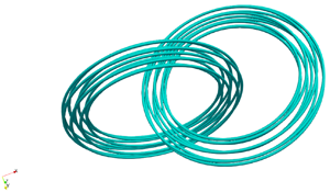
  ${\mathcal {V}}$ is the system's volume, is not a flow invariant. An example of such a flow is the dissipative dynamics of two vortex rings in the Hopf link configuration (Aref & Zawadski Reference Aref and Zawadski1991; Brady, Leonard & Pullin Reference Brady, Leonard and Pullin1998; Kivotides & Leonard Reference Kivotides and Leonard2003a). Initially, the vortex lines within the tubes are unlinked and untwisted. Although the flow outside the tube cores is essentially inviscid, the link is destroyed and topology changes via a dissipative vortex reconnection. Moffatt (Reference Moffatt1969, Reference Moffatt2014) and Ricca & Moffatt (Reference Ricca and Moffatt1992) indicated that this topological change is directly related to helicity, by deriving an intriguing relation between $\mathcal {H}$, a physical quantity, and topological measures of a system of $N$ vortex tubes:
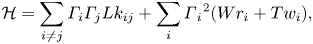 \begin{equation} \mathcal{H}=\sum_{i \neq j}{\varGamma_i \varGamma_j Lk_{ij}}+\sum_i{\varGamma{_i}^{2} (Wr_i+Tw_i)}, \end{equation}
where  $\varGamma _i$ is the circulation of tube $i$,
$i$,  $Lk_{ij}$ is the Gauss linking number of tubes $i$ and $j$, and $Wr_i$ and $Tw_i$ are, correspondingly, the writhe and twist of tube $i$. The sum of $Wr_i$ and $Tw_i$ is the Cǎlugǎreanu self-linking number ${SLk}_i$, which measures the degree of knottedness of single closed tubes, and, according to Cǎlugǎreanu's theorem (Cǎlugǎreanu Reference Cǎlugǎreanu1961; Moffatt & Ricca Reference Moffatt and Ricca1992), is a topological invariant. Helpful discussions of these topological concepts in the contexts of physics applications are available in Scheeler et al. (Reference Scheeler, van Rees, Kedia, Kleckner and Irvine2017) and Berger & Prior (Reference Berger and Prior2006). Remarkably, the formula relates helicity with linking measures, which are directly connected with curve geometry (§ 4 in this paper). This is because helicity is a measure of streamline right- or left-handedness, and this is exactly what the $Lk$ number measures in a geometry, since for a system of $i$ curves, $Lk=\sum _i w_i/2$, i.e. $Lk$ is a summation over weights of all crossings between different curves. The crossings are counted on a two-dimensional projection of the curve system along an arbitrary direction, and their weights are $w=+1$ for each right-handed crossing and $w=-1$ for each left-handed crossing. On the helicity side, the counting becomes an integral, and the weights are automatically encoded in the signs of the inner products between velocity and vorticity. The circulation factors in the Moffatt & Ricca formula are then a dimensional book-keeping, as implied by the Biot–Savart law. Recently, new important developments indicated derivation of the skein relations of the HOMFLYPT polynomial for ideal fluid knots from helicity (Liu & Ricca Reference Liu and Ricca2015). Similar associations of helicity with other knot polynomials (Sossinsky Reference Sossinsky2004) or Vassiliev invariants above the lowest order (Mostovoy, Chmutov & Duzhin Reference Mostovoy, Chmutov and Duzhin2017) are highly desirable. It would certainly be important to find new conserved flow quantities that correspond to these types of invariants.
The Moffatt & Ricca formula offers new points of view for physics investigations. Indeed, let us consider, without loss of generality, a case where the ring cores (that set the characteristic scale of reconnection area, hence, also of dissipative effects) are much smaller than the ring diameters. Since the latter plausibly indicate the scale where most of net helicity ought to reside, one argues that, at sufficiently high Reynolds numbers, and correspondingly small reconnection durations, a small-scale dissipative effect (reconnection) ought not to alter significantly a large-scale quantity (helicity). To transfer intuition from turbulence physics, Taylor-scale dissipative processes destroy, at any time, a small part of the kinetic energy of the large, energy-containing motions. Such arguments would suggest that, at high Reynolds number ( $Re \gg 1$), for helicity to be approximately the same before and after reconnection, the Moffatt & Ricca formula needs to predict a change of helicity from one type of topological measure ( $Lk_{ij}$) to another ( $Wr_i+Tw_i$). A topological justification of the same conclusion was offered by Pfister & Gekelman (Reference Pfister and Gekelman1990). Employing ribbons for theoretical illustration, they argued that $Lk$ becomes $Tw$ during reconnection. We show here that, in our vortex-dynamical model, $Lk$ becomes $Wr$, which is something similar, since Pfister & Gekelman (Reference Pfister and Gekelman1990) and Moffatt & Ricca (Reference Moffatt and Ricca1992) indicate how twist (formed by helical winding of one ribbon edge about the other) can be transformed to writhe (corresponding to self-intersections of the ribbon centreline in a two-dimensional projection of it) via continuous transformations. This interchangeability of $Wr$ and $Tw$ is implied by the topological nature of $SLk$, and can even be realized when topological calculations that refer to the same geometry employ different view angles (Klenin & Langowski Reference Klenin and Langowski2000).
These matters were first experimentally clarified by Scheeler et al. (Reference Scheeler, Kleckner, Proment, Kindlmann and Irvine2014), who measured the post-reconnection  $Wr$ and showed that it was comparable with the initial $Lk$ value. Their experimental techniques did not allow them to measure directly the post-reconnection twist, but the measured writhe values were adequate for demonstrating the relatively small effect of the reconnection on helicity levels. There are two important remarks implied by their results: (a) small helicity changes can correspond to marked changes in topological measures, i.e. for similar pre- and post-reconnection helicity levels, all initial linking becomes writhe and twist, and (b) in the spirit of the physical arguments above, $Re$ must be high. Indeed, $Re \sim 2 \times 10^4$ in the experiment of Scheeler et al. (Reference Scheeler, Kleckner, Proment, Kindlmann and Irvine2014). At sufficiently small $Re$, the link dynamics would tend to create writhe and twist, but, in the absence of adequately large inertia, the latter is overwhelmingly damped by viscosity, a process providing a topological interpretation of helicity dissipation.
The purpose of this work is to theoretically probe the high- $Re$ helicity and topological dynamics of vortex links. There are three key aspects of our contribution. (a) We employ a discrete, yet finite-core, vortex-dynamical model of Hopf links, which corresponds to the limit of high-Reynolds-number vortex dynamics. In this respect, we took advantage of methods originating in quantum fluid dynamics (Kivotides Reference Kivotides2018b; Galantucci et al. Reference Galantucci, Baggaley, Parker and Barenghi2019), but adapted to Navier–Stokes vortex dynamics (Kivotides & Leonard Reference Kivotides and Leonard2003a), and successfully applied to high-Reynolds-number turbulence (Kivotides & Leonard Reference Kivotides and Leonard2004a,Reference Kivotides and Leonardb, Reference Kivotides and Leonard2003b), magnetohydrodynamics (Kivotides, Mee & Barenghi Reference Kivotides, Mee and Barenghi2007b) and solid–fluid dynamics (Kivotides et al. Reference Kivotides, Barenghi, Mee and Sergeev2007a). These references include, among others, comparisons between quantum and classical vortex dynamics, details about the reconnection algorithm and the effects on performance of its various parameters, systematic comparison with numerical solutions of the Navier–Stokes equations, reproduction of key Navier–Stokes turbulence spectra scalings, turbulence kinematics and geometrical physics, as well predictions of kinematic magnetohydrodynamic dynamo spectra and depictions of particle–vortex interactions in turbulent suspensions. Our reconnection algorithm originates in the work of Schwarz on quantum vortex dynamics Schwarz (Reference Schwarz1985). However, there are important differences between quantum and classical vortex dynamics. The former case deals with discrete vortex lines of singular vorticity and constant (in all flow cases) circulations, whilst the second involves finite, dynamic core tubes with continuous vorticity distributions and freely varying circulations. During tube reconnection, many vortex lines (which discretize the tube vorticity) can reconnect in close succession. It is important to preserve tube integrity during this process. This requires a careful choice of the vortex approach distance upon which topological surgery takes place. In the calculations presented here, we have chosen the smallest distance that does not lead to unphysical results during tube stretching dynamics, as are erroneous $Lk$ increments before the onset of reconnections. To be more specific, there is a different approach to reconnections in the two cases: in quantum fluids, reconnections are performed when two vortices approach closer than a computational reconnection distance (CRD) which is of the order of their numerical discretization length. Small CRD changes do not lead to large changes in the results. This is because, in quantum fluids, there are no finite-core vortex tubes, but only isolated line vortices (known as topological defects in quantum field theory). In classical fluids, however, CRD choice follows a more elaborate, iterative procedure. For the particular vortex core and circulation in the initial conditions, we start by employing a CRD of the order of the numerical discretization along the vortex contours, and we perform a series of computations with decreasing CRD. The main concerns are to keep tube integrity during reconnection, and, at the same time, not to have unphysical topological changes before reconnection onset. The final CRD chosen is the smallest CRD that satisfies both both of the above requirements. The details of the corresponding series of numerical calculations and their accompanying CRD values are discussed in the computational methodology section. Moreover, in the present context, we also apply the model of Kivotides & Leonard (Reference Kivotides and Leonard2003a) with constant cores, i.e. without diffusive core growth; hence the sole physical effect of reconnections is to effect topological change. In this way, our vortices are numerical analogues of reconnecting, vortex lines in the high-Reynolds-number limit. (b) In contrast with the standard spectra of velocity or vorticity vector fields which refer to the squares (energy and enstrophy) of these quantities, we employ methods for the computation of the spectra of the actual helicity values. Hence, our helicity spectra inform not only about the scale-by-scale partition of helicity, but also about the sign of the latter. Employing these methods, we accurately probe the interscale helicity transfer processes. (c) We calculate the topological measures in the Moffatt & Ricca formula with great precision, by transferring to vortex dynamics robust topology measuring methods first developed in the context of DNA biopolymer studies. After discussing the mathematical details of each of these tools, we apply them to vortex-link dynamics and discuss the resulting physics.
2. Discrete model of reconnecting vortex tubes
In order to theoretically match the high Reynolds numbers in experiments, and, in fact, to do even better in this respect, we note that in the limit of  $Re \gg 1$ vortex-link dynamics, one expects a small (in comparison with the total energy content) amount of dissipation, whose main role is to facilitate vortex reconnection. These physical requirements are matched by the mesoscopic model of quantum vortex dynamics employed in superfluids research (Kivotides Reference Kivotides2018b, Reference Kivotides2014). Whilst at microscopic scales an (inviscid) supefluid flows under the influence of its quantum stress that controls fluid density and effects reconnections (Legget Reference Legget2006), at mesoscopic scales a superfluid behaves like an incompressible fluid with phenomenological reconnections (Feynman Reference Feynman1955; Schwarz Reference Schwarz1985; Kivotides Reference Kivotides2014). In this context, the vortices are slender filaments, and vorticity is distributed within their finite cores via suitable smoothing kernels:
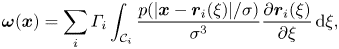 \begin{equation} \boldsymbol{\omega}(\boldsymbol{x}) = \sum_i \varGamma_i \int_{\mathcal{C}_i} \frac{p(|\boldsymbol{x} - \boldsymbol{r}_i(\xi)|/\sigma)}{\sigma^3}\frac{\partial \boldsymbol{r}_i(\xi)}{\partial \xi}\,\textrm{d} \xi, \end{equation}
where the circulation of tube  $i$ is $\varGamma _i$ and its centreline $\mathcal {C}_i$ is given by the space curve $\boldsymbol {r}_i(\xi )$, where $\xi$ is the arclength parametrization of curve $\mathcal {C}_i$. The function $p$ determines the vorticity distribution over the core of the tube having an effective radius of $\sigma$, and facilitates stable numerical calculations. The calculations are performed with the Gaussian kernel of Winckelmans & Leonard (Reference Winckelmans and Leonard1993):
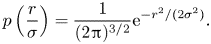 \begin{equation} p \left(\frac{r}{\sigma} \right) = \frac{1}{(2 {\rm \pi})^{{3}/{2}}} \textrm{e}^{-r^2/(2\sigma^2)}. \end{equation}
Inserting the above definition of vorticity in the Biot–Savart integral reduces the latter to a sum of line integrals over each filament centreline contour:
 \begin{equation} \boldsymbol{u}(\boldsymbol{x})=-\sum_i \frac{\varGamma_i}{4 {\rm \pi}} \int_{\mathcal{C}_i}\,\textrm{d}\xi \frac{Q(\phi)}{(\sqrt{2} \sigma)^3} \frac{\partial \boldsymbol{r}_i(\xi)}{\partial \xi} \times (\boldsymbol{r}_i(\xi)-\boldsymbol{x}), \end{equation}
where function  $Q(\phi )$ (with $\phi =|\boldsymbol {r}_i-\boldsymbol {x}|/\sqrt {2} \sigma$) depends on the particular smoothing kernel employed. For the Gaussian kernel case, it is (Leonard Reference Leonard1985; Winckelmans & Leonard Reference Winckelmans and Leonard1993)
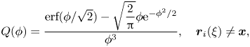 \begin{gather} Q(\phi)=\frac{\textrm{erf}(\phi/\sqrt{2})-\sqrt{\dfrac{2}{\rm \pi}} \phi \textrm{e}^{-\phi^2/2}}{\phi^3},\quad \boldsymbol{r}_i(\xi)\neq\boldsymbol{x}, \end{gather}
 \begin{gather}Q(\phi)=\sqrt{\frac{2}{9 {\rm \pi}}},\quad \boldsymbol{r}_i(\xi)=\boldsymbol{x}. \end{gather}
There are some important features: by employing the smoothing kernel, we transform line vortices to vortex tubes. This is very much in agreement with the derivation of the Moffatt & Ricca formula (Moffatt & Ricca Reference Moffatt and Ricca1992) where both writhe and twist are forms of self-linking involving the vortex lines within single tubes. Pfister & Gekelman (Reference Pfister and Gekelman1990), Moffatt & Ricca (Reference Moffatt and Ricca1992) and Scheeler et al. (Reference Scheeler, Kleckner, Proment, Kindlmann and Irvine2014) offer nice illustrations of this point. Hence, our model entails both  $Lk$ and $Wr$ physics. On the other hand, since the numerical tubes are not capable of core deformation, by default, there is no $Tw$ in our flow field.
It is important to discuss this last point to accurately embed our method within the general context of topological vortex physics. In the context of single vortex tube dynamics, there are two relevant topological quantities:  $Wr$ and $Tw$ (Asgari-Targhi & Berger Reference Asgari-Targhi and Berger2009). They measure the topology of the continuum bundle of vortex lines that comprise the tube, with each line providing infinitesimal contribution to the total flux. So in continuum physics, we need an infinity of vortex lines to model each of the two finite tubes that comprise a Hopf link. In our numerical approach, we discretize the finite-core tubes into bundles of finite number of vortices. The cores of the latter are (by construction) non-deformable, and do not include twisted vortex lines. In other words, there are no physically dynamical cores associated with our discrete vortices, whose evolution we can meaningfully track in time. At every time step, the line vortices are ‘dressed’ with (constant) numerical cores, which, once the smoothed velocity field is computed, are discarded, and do not propagate to the next time step. As mentioned above, this smoothing includes $Wr$ physics but not $Tw$ physics. Our results are physically consistent, since, further on, we demonstrate an excellent correspondence between topological measures based on the discrete vortices (excluding $Tw$) and flow field helicity values. Attributing $Tw$ to our discrete vortices would add to topology a feature that is not present in the flow field. This would, by default, invalidate our computation, since the helicity spectra, for example, would not correspond to the topological helicity values.
Certainly, by defining an effective core based on the boundaries of numerical vortex bundles, one can compute  $Tw$ values for the macroscopic tubes, and, by considering the contour of the bundle-centreline vortex, also $Wr$ values, if needed. It is only the $Tw$ of the discrete vortices that is not modelled within the numerical approximation. So let us discuss in detail how our numerical method tackles vortex-dynamical processes that involve $Tw$ dynamics. Take for example (Asgari-Targhi & Berger Reference Asgari-Targhi and Berger2009) the case of a circular vortex tube that is given a large-scale turn so that it approaches a figure-of-eight shape. Since there is a variation of $Wr$, helicity conservation implies an opposite sign variation of $Tw$. Such a situation is handled in our method by discretizing the original tube into a bundle of elementary ( $Tw$-free) vortices. During the figure-of-eight formation, the vortices in the tube get twisted generating $Tw$ in the macroscopic tube, whilst the computation of the macroscopic tube $Wr$ is based on the vortex at the bundle centreline. On the other hand, by decreasing the circulation of discrete vortices and the discretization length along vortex contours, we can increase the accuracy and resolution of our calculations as desired.
On another front, the phenomenological (jump process) nature of the reconnections in our system (Kivotides Reference Kivotides2014) is fully compatible with the discrete character of topological change, and, indeed, Pfister & Gekelman (Reference Pfister and Gekelman1990) employ a similar jump process in their demonstration of helicity conservation during ribbon reconnection. In conclusion, we expect that, due to lack of dissipation, and within the accuracy levels of our vortex-dynamics methodology, helicity is going to be conserved, modulo transient, spurious physical effects due to the discontinuous nature of reconnections in our model, yet the topological dynamics will be accurate, and helicity-related conclusions qualitatively correct. On the other hand, we gain important insight into high-Reynolds-number vortex dynamics.
To cross-check our calculations, we compute helicity with both vortex dynamics and topological formulae. Within the former (Winckelmans & Leonard Reference Winckelmans and Leonard1993), total vorticity  $\mathcal {H}$ is given by
 \begin{equation} \mathcal{H}=\sum_{i,j} \varGamma_i \varGamma_j \iint\frac{q_{\sigma}(\boldsymbol{r}_i-\boldsymbol{r}_j)}{\vert\boldsymbol{r}_i-\boldsymbol{r}_j\vert} \left[(\boldsymbol{r}_i-\boldsymbol{r}_j) \boldsymbol{\cdot } \left(\frac{\partial \boldsymbol{r}_i(\xi)}{\partial \xi} \times \frac{\partial \boldsymbol{r}_j(\xi^{\prime})}{\partial \xi^{\prime}} \right) \right]\,\textrm{d}\xi\,\textrm{d}{\xi^{\prime}}, \end{equation}
where  $q_{\sigma }(\boldsymbol {r})=q(\vert \boldsymbol {r} \vert /\sigma )$ and
 \begin{equation} q(\rho)=\int_0^{\rho} p(t) t^2\,\textrm{d}t. \end{equation}
 In discretizing actual Navier–Stokes vortex tubes in terms of elementary vortex filaments, we employ the methods of Knio & Ghoniem (Reference Knio and Ghoniem1990) and Winckelmans & Leonard (Reference Winckelmans and Leonard1993). Although our approach follows closely that of Winckelmans & Leonard (Reference Winckelmans and Leonard1993), the presence of reconnections in our model imposes strict discretization constraints, not present in previous works. To set up a discretization of a ring-like vortex tube, we choose the ‘quantum’ of circulation, i.e. the circulation  $\varGamma _i$ of each elementary vortex $i$, which is set equal to $\kappa$ for all vortices, and the circulation $\varGamma _m$ of the ‘macroscopic’ tube. The ratio $n_v=\varGamma _m/\kappa$ can be thought of as the number of ‘grid points’ that are required to approximate the internal dynamics of the macroscopic vortex tube. The idea in Knio & Ghoniem (Reference Knio and Ghoniem1990) and Winckelmans & Leonard (Reference Winckelmans and Leonard1993) is to discretize the macroscopic tube into a sequence of $n_c$ layers (toroidal shells), each one containing $8 n_c$ elementary vortices. Hence, $n_v$ determines the number of discretization layers. By taking the outer radius of each layer (measured from the tube centreline and on a plane normal to the latter) equal to $(2 n_c+1) r_{\ell }$, and having the elementary vortices passing through each layer along a perimeter of radius $r_c=(1+12 n_c^2/6 n_c) r_{\ell }$ (also measured from the tube centreline), we place each vortex at the centre of an area ${\rm \pi} r_{\ell }^2={\rm \pi} R_t^2/n_v$. Here, $R_t$ is the tube core radius. Notably, in this construction, the macroscopic tube centreline is always occupied by a line vortex. A central point is that, in the phenomenological reconnections model, the elementary vortices reconnect when they approach closer than $\delta \approx 0.1 \Delta \xi$, where $\Delta \xi$ is the discretization length along the vortices. We need the vortices to reconnect as a result of vortex-dynamically generated configurations, and not artificially, due to small distances from each other in the initial conditions. Hence, $\delta =0.1 \Delta \xi$ must be significantly smaller than $r_{\ell }$ (in the calculations it is smaller by a factor of $4$), and this imposes a lower resolution limit that, in turn, determines computational complexity levels. Computational complexity scales with the $N^2$ operations required by Biot–Savart interactions (where $N$ is the number of numerical vortex segments). To double the Reynolds number, we need to double the bundle circulation, hence also double the number of line vortices in the system. Keeping resolution the same, the number of vortex segments becomes, in this way, $2 N$, and thus the computational complexity increases by a factor of $4$.
$4$.
3. Helicity spectra for Navier–Stokes and vortex-dynamical formulations
3.1. Navier–Stokes spectra
We aim to derive here a formula for the spectrum of helicity (rather than its square). We first consider the field theoretic case, before the vortex-dynamics one. The total helicity  $\mathcal {H}$ is given by
 \begin{equation} \mathcal{H} = \int \boldsymbol{u}(\boldsymbol{x}) \boldsymbol{\cdot} \boldsymbol{\omega}(\boldsymbol{x})\,\textrm{d}\kern0.5pt \boldsymbol{x}. \end{equation}
Substituting  $\boldsymbol {u}$ and $\boldsymbol {\omega }$ with their inverse Fourier transforms (we use $1/2 {\rm \pi}$ and $\exp ({- \textrm {i} \boldsymbol {k} \boldsymbol {\cdot } \boldsymbol {x}})$ factors when taking the inverse transform, and we define $k=2 {\rm \pi}/\ell$, with $\ell$ a length scale) we have
 \begin{equation} \mathcal{H} = \left(\frac{1}{2 {\rm \pi}} \right)^6 \iiint \hat{\boldsymbol{u}}(\boldsymbol{k}) \boldsymbol{\cdot} \hat{\boldsymbol{\omega}}(\boldsymbol{k'}) \exp\left({- \textrm{i} \boldsymbol{k} \boldsymbol{\cdot} \boldsymbol{x} - \textrm{i} \boldsymbol{k'} \boldsymbol{\cdot} \boldsymbol{x}}\right)\,\textrm{d}\kern0.5pt \boldsymbol{x}\,\textrm{d} \boldsymbol{k}\,\textrm{d} \boldsymbol{k'}. \end{equation}
Integration over  $\boldsymbol {x}$ produces the delta function $(2 {\rm \pi})^3 \delta (\boldsymbol {k} + \boldsymbol {k'})$. In addition, we have that
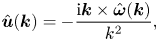 \begin{equation} \hat{\boldsymbol{u}}(\boldsymbol{k}) = -\frac{\textrm{i} \boldsymbol{k} \times \hat{\boldsymbol{\omega}}(\boldsymbol{k})}{k^2} , \end{equation}
and therefore (3.3) becomes
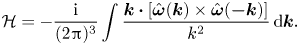 \begin{equation} \mathcal{H} = -\frac{\textrm{i}}{(2 {\rm \pi})^3} \int \frac{\boldsymbol{k} \boldsymbol{\cdot} \left[\hat{\boldsymbol{\omega}}(\boldsymbol{k}) \times \hat{\boldsymbol{\omega}}(\boldsymbol{- k}) \right] }{k^2}\,\textrm{d}\boldsymbol{k}. \end{equation}
Using spherical coordinates in  $\boldsymbol {k}$-space, i.e. $\textrm {d}\boldsymbol {k} = \textrm {d}\boldsymbol {\varOmega }_k k^2\,\textrm {d}k$ and transforming back to real space, (3.4) becomes
 \begin{equation} \mathcal{H} = -\frac{\textrm{i}}{(2 {\rm \pi})^3} \iiint \left( \int \boldsymbol{k} \boldsymbol{\cdot} \left[\boldsymbol{\omega}(\boldsymbol{x}) \times \boldsymbol{\omega}(\boldsymbol{x'}) \right] \exp\left({ \textrm{i} \boldsymbol{k} \boldsymbol{\cdot} (\boldsymbol{x} - \boldsymbol{x'})}\right) \right)\,\textrm{d}\boldsymbol{\varOmega}_k\,\textrm{d}\kern0.5pt \boldsymbol{x}\,\textrm{d}\boldsymbol{x'}\,\textrm{d}k. \end{equation}
Integration over  $\boldsymbol {\varOmega }_k$ is accomplished simply by assuming $\boldsymbol {x} - \boldsymbol {x'}$ is in the polar direction so that
 \begin{align} \mathcal{H} = -\frac{\textrm{i}}{(2 {\rm \pi})^2} \iiint \left( \int^1_{- 1} k \mu \frac{\boldsymbol{x} - \boldsymbol{x'}}{|\boldsymbol{x} - \boldsymbol{x'}|} \boldsymbol{\cdot} \left[\boldsymbol{\omega}(\boldsymbol{x}) \times \boldsymbol{\omega}(\boldsymbol{x'}) \right] \exp\left({ \textrm{i} k \mu |\boldsymbol{x} - \boldsymbol{x'}|}\right)\,\textrm{d}\mu \right)\,\textrm{d}\kern0.5pt \boldsymbol{x}\,\textrm{d}\boldsymbol{x'}\,\textrm{d}k, \end{align}
where  $\mu$ is the cosine of the angle between $\boldsymbol {k}$ and $\boldsymbol {x} - \boldsymbol {x'}$. Integration over $\mu$ in (3.6) gives
 \begin{equation} \mathcal{H} = -\frac{1}{2 {\rm \pi}^2} \int_k \iint k \frac{\textrm{d}}{\textrm{d}k}\left( \frac{\sin(k |\boldsymbol{x} - \boldsymbol{x'}|}{k |\boldsymbol{x} - \boldsymbol{x'}|}\right) \frac{\boldsymbol{x} - \boldsymbol{x'}}{|\boldsymbol{x} - \boldsymbol{x'}|^2} \boldsymbol{\cdot} \left[\boldsymbol{\omega}(\boldsymbol{x}) \times \boldsymbol{\omega}(\boldsymbol{x'}) \right]\,\textrm{d}\kern0.5pt \boldsymbol{x}\,\textrm{d}\boldsymbol{x'}\,\textrm{d}k. \end{equation}
Thus we can define the helicity spectrum  $\hat {\mathcal {H}}(k)$ as
 \begin{equation} \hat{\mathcal{H}}(k) = -\frac{1}{2 {\rm \pi}^2} \iint k \frac{\textrm{d}}{\textrm{d}k}\left( \frac{\sin(k |\boldsymbol{x} - \boldsymbol{x'}|}{k |\boldsymbol{x} - \boldsymbol{x'}|}\right) \frac{\boldsymbol{x} - \boldsymbol{x'}}{|\boldsymbol{x} - \boldsymbol{x'}|^2} \boldsymbol{\cdot} \left[\boldsymbol{\omega}(\boldsymbol{x}) \times \boldsymbol{\omega}(\boldsymbol{x'}) \right]\,\textrm{d}\kern0.5pt \boldsymbol{x}\,\textrm{d}\boldsymbol{x'}, \end{equation}
so that
 \begin{equation} \mathcal{H} = \int^\infty_0 \hat{\mathcal{H}}(k)\,\textrm{d}k. \end{equation}
Indeed integration of  $\hat {\mathcal {H}}(k)$ gives
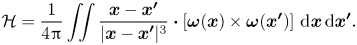 \begin{equation} \mathcal{H} = \frac{1}{4 {\rm \pi}} \iint\frac{\boldsymbol{x} - \boldsymbol{x'}}{|\boldsymbol{x} - \boldsymbol{x'}|^3} \boldsymbol{\cdot} \left[\boldsymbol{\omega}(\boldsymbol{x}) \times \boldsymbol{\omega}(\boldsymbol{x'}) \right]\,\textrm{d}\kern0.5pt \boldsymbol{x}\,\textrm{d}\boldsymbol{x'}. \end{equation}
3.2. Vortex-dynamics spectra
The helicity spectrum formula for the vortex-dynamical model is
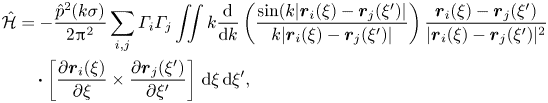 \begin{align} \hat{\mathcal{H}} &= -\frac{\hat{p}^2(k \sigma)}{2 {\rm \pi}^2} \sum_{i,j} \varGamma_i \varGamma_j \iint k \frac{\textrm{d}}{\textrm{d}k}\left( \frac{\sin(k |\boldsymbol{r}_i(\xi) - \boldsymbol{r}_j(\xi')|}{k |\boldsymbol{r}_i(\xi) - \boldsymbol{r}_j(\xi')|}\right) \frac{\boldsymbol{r}_i(\xi) - \boldsymbol{r}_j(\xi')}{|\boldsymbol{r}_i(\xi) - \boldsymbol{r}_j(\xi')|^2}\nonumber\\ &\quad\boldsymbol{\cdot} \left[ \frac{\partial \boldsymbol{r}_i(\xi)}{\partial \xi} \times \frac{\partial \boldsymbol{r}_j(\xi')}{\partial \xi'} \right]\,\textrm{d}\xi\,\textrm{d}\xi', \end{align}
where the function  $\hat {p}$ corresponding to the employed Gaussian kernel is $\hat {p}(k \sigma )=\textrm {e}^{-{(k \sigma )}^2/2}$. Note that $\hat {p}(0)=1$. Both formulae have an apparent singularity when considering the self-contribution to helicity of a field or vortex point. However, by calculating analytically the derivative in (3.12)
 \begin{equation} k \frac{\textrm{d}}{\textrm{d}k}\left(\frac{\sin(k |\boldsymbol{r}_i(\xi) - \boldsymbol{r}_j(\xi')|}{k |\boldsymbol{r}_i(\xi) - \boldsymbol{r}_j(\xi')|}\right)= \cos(k |\boldsymbol{r}_i(\xi) - \boldsymbol{r}_j(\xi')|)-\frac{\sin (k |\boldsymbol{r}_i(\xi) - \boldsymbol{r}_j(\xi')|)}{k |\boldsymbol{r}_i(\xi) - \boldsymbol{r}_j(\xi')|}, \end{equation}
employing L'H $\check{{\rm o}}$pital's rule to compute the limit $\textrm {sin}x/x$ when $x \rightarrow 0$ and expanding the cross-product ${\partial \boldsymbol {r}_i(\xi )}/{\partial \xi } \times {\partial \boldsymbol {r}_j(\xi ')}/{\partial \xi '}$ around $\xi$ when $\xi '\rightarrow \xi$, one can easily deduce that the self-contributions are equal to zero.
For an alternative derivation of the helicity spectrum based on two-point correlation functions and applied to magnetohydrodynamic dynamo physics, see Asgari-Targhi & Berger (Reference Asgari-Targhi and Berger2009).
4. Methods for calculating linking and writhe
To compute topological dynamics, we only need calculate  $Lk$ and $Wr$, since, as mentioned above, $Tw$ in the Moffatt & Ricca formula is zero by default in our vortex dynamics. For completeness, we discuss, however, how $Tw$ has been taken into account in other vortex-dynamics studies (Zuccher & Ricca Reference Zuccher and Ricca2015, Reference Zuccher and Ricca2017; Hänninen, Hietale & Salman Reference Hänninen, Hietale and Salman2016). Hänninen et al. (Reference Hänninen, Hietale and Salman2016) study $Tw$ by constructing macroscopic tubes from single quantum vortices, which are bundled together and endowed with Kelvin wave excitations that are mild enough to allow the tubes to remain coherent for finite period of time. By considering a ribbon based on the centreline of such macroscopic tubes, $Tw$ can be meaningfully defined and measured. However, this approach is meaningful only as long as the tube remains coherent. Our macroscopic tubes undergo reconnections and other non-trivial dynamics that do not preserve tube coherence. Hence, by basing our topological analysis on $Lk$ and $Wr$ of elementary vortices, we perform a more general analysis that does not rely on assumptions of tube integrity. On the other hand, the works of Zuccher & Ricca (Reference Zuccher and Ricca2015, Reference Zuccher and Ricca2017) and Kedia et al. (Reference Kedia, Kleckner, Scheeler and Irvine2018) indicate that $Tw$ can meaningfully be ascribed to a discrete quantum vortex, but this refers to core dynamics governed by quantum stresses active at microscopic scales, and are not relevant to mesoscopic scales or to classical vortex dynamics, where quantum stresses are absent. In other words, the $Tw$ of Zuccher & Ricca (Reference Zuccher and Ricca2015, Reference Zuccher and Ricca2017) and Kedia et al. (Reference Kedia, Kleckner, Scheeler and Irvine2018) is not relevant to classical fluid dynamics, and that of Hänninen et al. (Reference Hänninen, Hietale and Salman2016) is entailed in the topology of the elementary vortex system.
We follow the method of Klenin & Langowski (Reference Klenin and Langowski2000), which was developed in the context of biopolymer studies, but can also be applied to vortex dynamics, by taking advantage of the discretization of each vortex into closed polygonal curves. Then, the total linking  $Lk=\sum _i \sum _j Lk_{ij}$ is the sum of all linking numbers $Lk_{ij}$ between possible vortex pairs $i$ and $j$, noting that $Lk_{ij}=Lk_{ji}$ and $Lk_{ii}\equiv 0$. Each specific linking number $Lk_{ij}$ is given by
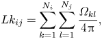 \begin{equation} Lk_{ij}=\sum_{k=1}^{N_i} \sum_{l=1}^{N_j} \frac{\varOmega_{kl}}{4 {\rm \pi}}, \end{equation}
where  $N_i$ and $N_j$ are the number of discretization segments of vortices $i$ and $j$, respectively. Here $\varOmega _{kl}/4 {\rm \pi}$ is the Gauss integral along segments $k$ and $l$, with $k$ and $l$ belonging to two different vortices. Integral $\varOmega _{kl}$ is computed in terms of four vectors: $\boldsymbol {r_1}$ and $\boldsymbol {r_2}$ corresponding to start and end points of segment $k$, and $\boldsymbol {r_3}$ and $\boldsymbol {r_4}$ corresponding to start and end points of segment $l$. By using $\boldsymbol {r_{ij}}\equiv \boldsymbol {r_j}-\boldsymbol {r_i}$, we have
 \begin{equation} \varOmega_{kl}=\varOmega^{*}_{kl} \textrm{sign}\left(\left(\boldsymbol{r_{34}} \times \boldsymbol{r_{12}}\right) \boldsymbol{\cdot} \boldsymbol{r_{13}}\right), \end{equation}
where
 \begin{equation} \varOmega^{*}_{kl}=\textrm{arcsin}\left(\boldsymbol{n_1} \boldsymbol{\cdot} \boldsymbol{n_2}\right)+\textrm{arcsin}\left(\boldsymbol{n_2} \boldsymbol{\cdot} \boldsymbol{n_3}\right)+ \textrm{arcsin}\left(\boldsymbol{n_3}\boldsymbol{\cdot}\boldsymbol{n_4}\right)+\textrm{arcsin}\left(\boldsymbol{n_4}\boldsymbol{\cdot}\boldsymbol{n_1}\right) \end{equation}
and
 \begin{align} \boldsymbol{n_1}=\frac{\boldsymbol{r_{13}} \times \boldsymbol{r_{14}}}{\vert \boldsymbol{r_{13}} \times \boldsymbol{r_{14}}\vert},\quad \boldsymbol{n_2}=\frac{\boldsymbol{r_{14}} \times \boldsymbol{r_{24}}}{\vert \boldsymbol{r_{14}} \times \boldsymbol{r_{24}}\vert},\quad \boldsymbol{n_3}=\frac{\boldsymbol{r_{24}} \times \boldsymbol{r_{23}}}{\vert \boldsymbol{r_{24}} \times \boldsymbol{r_{23}}\vert},\quad \boldsymbol{n_4}=\frac{\boldsymbol{r_{23}} \times \boldsymbol{r_{13}}}{\vert \boldsymbol{r_{23}} \times \boldsymbol{r_{13}}\vert}. \end{align}
The  $Wr_i$ of a single curve $i$ is similarly computed:
 \begin{equation} Wr_i=2 \sum_{k=2}^{N_i} \sum_{l < k} \frac{\varOmega_{kl}}{4 {\rm \pi}}, \end{equation}
where relations  $\varOmega _{kl}=\varOmega _{lk}$ and $\varOmega _{k(k+1)}=\varOmega _{kk}\equiv 0$ apply.
5. Topology and helicity in vortex link dynamics
5.1. Vortex-dynamical calculation
The initial conditions consist of two tubes in Hopf link configuration (figure 1a). To limit computational complexity, we have chosen  $n_v=9$. Based on tube centreline radius $R_c$ and tube circulation $\varGamma _m$, we define a unit time $t_u=R_c^2/\varGamma _m$. Helicity values are normalized with $\kappa ^2$, so that they can be directly compared with $Wr$ or $Lk$ values. The effective tube radius is $R_t=0.2 R_c$.Due to their Biot–Savart interactions, the tubes are stretched as they locally align with each other on the road to reconnection (figure 1b). The latter takes place discontinuouly, as a sequence of pair reconnections between elementary vortices belonging to different tubes (figure 1b,c). Once the stretched reconnection ‘bridge’ disappears (figure 1d), the system evolves into a blob of fluctuating vorticity (figure 1e,f), and by the time of $3.5 {t_u}$, the initial configuration is no longer discernible. Due to the complexity of the vortex tangle comprising the resulting blob of vorticity, there is continuing reconnections activity between the elementary vortices.

Figure 1. A vortex link made of discretized tubes reconnects and evolves into a blob of fluctuating vorticity. From (a) to (f) the times are:  $0$,
$0$,  $0.42$, $0.56$, $1.12$, $2.24$ and $3.5$ ( $t_u$ units).
To check the consistency between vortex dynamics and topology, we have computed helicity employing both its Moffatt & Ricca and vortex-dynamic (relation (3.11)) formulae. In all of following results, helicity values are normalized by dividing with appropriate  $\varGamma ^2$ factors, so that the initial helicity value of the vortex link is equal to two, in both vortex-dynamical and Navier–Stokes calculations. There is very good agreement (figure 2a) between the two sets of values, except close to the reconnection threshold, where vortex dynamics is not as accurate as topology. This difference between vortex-dynamical and topological evaluations is due to the fact that topological helicity evaluation does not depend on the geometry of the linked lines, and hence it is exact for all resolutions, which is not the case for the vortex-dynamical evaluation. Hence, in the latter case, results can only approximate the exact (topological) helicity in direct correspondence with the employed resolution. Taking into account that we have a link involving nine pairs of vortices, we expect $Lk=162$ at $t=0$, which is our topological result, which is matched exactly by the vortex-dynamical helicity value (figure 2b). As expected, $Lk$ remains constant until the onset of reconnections. Since our vortex dynamics employs topological (i.e. cut and glue) reconnections (Pfister & Gekelman Reference Pfister and Gekelman1990), and vortex evolution obeys the Euler equations, there is no dissipation in our system (which is why we propose it as an appropriate model of high-Reynolds-number vortex dynamics). Hence, in the limit of very high resolution, when reconnections are pointwise and occur upon vortex contact, we expect helicity to be conserved, and this, indeed, is indicated by the results, after a transient of duration $\sim 0.5 {t_u}$. This transient is an artifact of the discontinuous (jump process) nature of reconnections in our calculation. This, in turn, is a result of the relatively coarse grid that we employ in order to tame computational complexity. In an ideal computation, the employed fine grid would resolve all possible small-scale processes and vortices would reconnect upon quasi-contact. In such a calculation, the instantaneous drop of $Lk$ upon reconnection would be fully compensated by an instantaneous rise of $Wr$. Our grid is not dense enough to capture this small-scale $Wr$, and hence it takes some time ( ${\sim }0.5 {t_u}$) for $Wr$ to attain its appropriate levels. To demonstrate this assertion, we zoomed in the reconnection zone of a link made of single vortices, employing a grid six times denser than the one employed in the vortex-bundle case. We found that, while the coarse grid gave post-reconnection $Wr$ equal to approximately 27 % of pre-reconnection $Lk$, the dense grid increased this value to 66 %. Notably (figure 2b), the post-reconnection helicity is not all $Wr$, since there is reconnection-driven, continuous $Lk$ formation/destruction activity. The corresponding reconnections are not related to the unlinking process, but take place within the emergent vortex blob. Their number depends on the employed reconnection criterion $\delta$, i.e. the distance of approach between two filaments whereupon a reconnection jump is performed. We have tried different calculations with $\delta =[0.10,0.15,0.25,0.50] \Delta \xi$. The corresponding helicity plateau values (i.e. after the transient induced by the reconnection jumps has ceased) are $[1,1.17,1.31,1.5] H_0$, where $H_0$ is the initial helicity value. The shown results correspond to the smallest physically acceptable $\delta$. Smaller $\delta$ values lead to (unphysical) $Lk$ value increments before the onset of reconnections, and larger $\delta$ values produce post-reconnection helicity levels that exceed the initial value. Hence, the smallest $\delta$ value producing physically acceptable reconnections implies also conservation of helicity. This is certainly an attractive feature of the model.
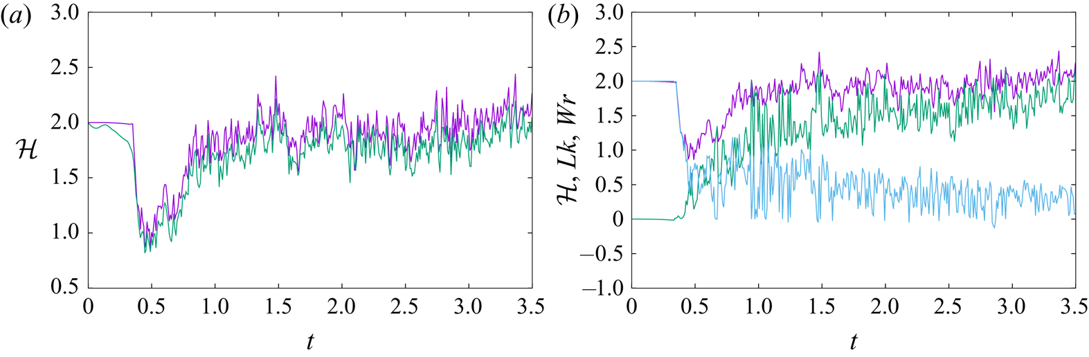
Figure 2. Vortex dynamics calculation. (a) Scaled helicity values obtained via the Moffatt & Ricca formula (upper curve) and directly from flow quantities (lower curve). (b) Scaled helicity values  $\mathcal {H}$ obtained via the Moffatt & Ricca formula (upper curve), $Wr$ (middle curve for post-reconnection times) and $Lk$ (lower curve for post-reconnection times).
At this point, our findings agree with physical and topological intuitions, and available experimental results. Indeed, as indicated in Pfister & Gekelman (Reference Pfister and Gekelman1990) and Scheeler et al. (Reference Scheeler, Kleckner, Proment, Kindlmann and Irvine2014), the initial  $Lk$ is mainly transformed into $Wr$, and the total helicity is conserved. To proceed further and understand better helicity structure, we look at helicity spectra $\hat {\mathcal {H}}(k)$. Remarkably, in a way reminiscent of energy spectra (Leonard Reference Leonard1985), the $\hat {\mathcal {H}}(k)$ of a link made of two single rings fluctuates between positive and negative values at all (resolvable) scales (figure 3a). We have checked that the integration of the spectra in wavenumber space gives exactly the total system helicity.When the link is made of vortex bundles instead of single vortices (figure 3b), there is a similar fluctuating behaviour at large scales, but the fluctuations die out fast. It can be concluded that the high $k$ helicity fluctuations are the signature of the combined potential vortex flow field around elementary vortices. By creating bundles of the latter, we create macroscopic tubes with finite-diameter, solid-body rotating cores, which (by default) have zero helicity. Indeed, it was easy to check that the cut-off of the spectrum coincides with the effective core of the macroscopic tubes. The spectra indicate that, as expected, there is a net positive helicity at large scales, but this net amount is the sum of alternating-sign helicity contributions at progressively smaller scales. What happens to helicity spectra as a result of the reconnection? There are two distinctive dynamical regimes. The first corresponds to the road to reconnection (figure 4a). There, the initial spectrum fluctuations are damped, and as total helicity is conserved, there is an elimination of significant negative helicity values. Hence, although in the ‘perfect’ link of the initial conditions the positive net helicity is the small difference between positive and negative values, just before reconnection there is mostly positive helicity in the system. This could very well be the spectral signature of stretched, reconnection bridge formation (figure 1b). After unlinking, we have an inverse cascade of helicity from small to large scales (figure 4b). This is an intriguing feature that reverses the pre-reconnection tendency of large-scale helicity damping. It corresponds to the formation of the homogenized vortex blob, with helicity concentrated at the scale of the (effective) blob diameter. This inverse cascade process is directly connected to the conservation of helicity in an inviscid system.
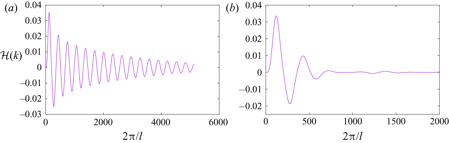
Figure 3. Vortex dynamics calculation. (a) Helicity spectra  $\hat {\mathcal {H}}(k)$ for a link composed of single line vortices. (b) Helicity spectra $\hat {\mathcal {H}}(k)$ for a link of tubes made of bundles of nine line vortices each.
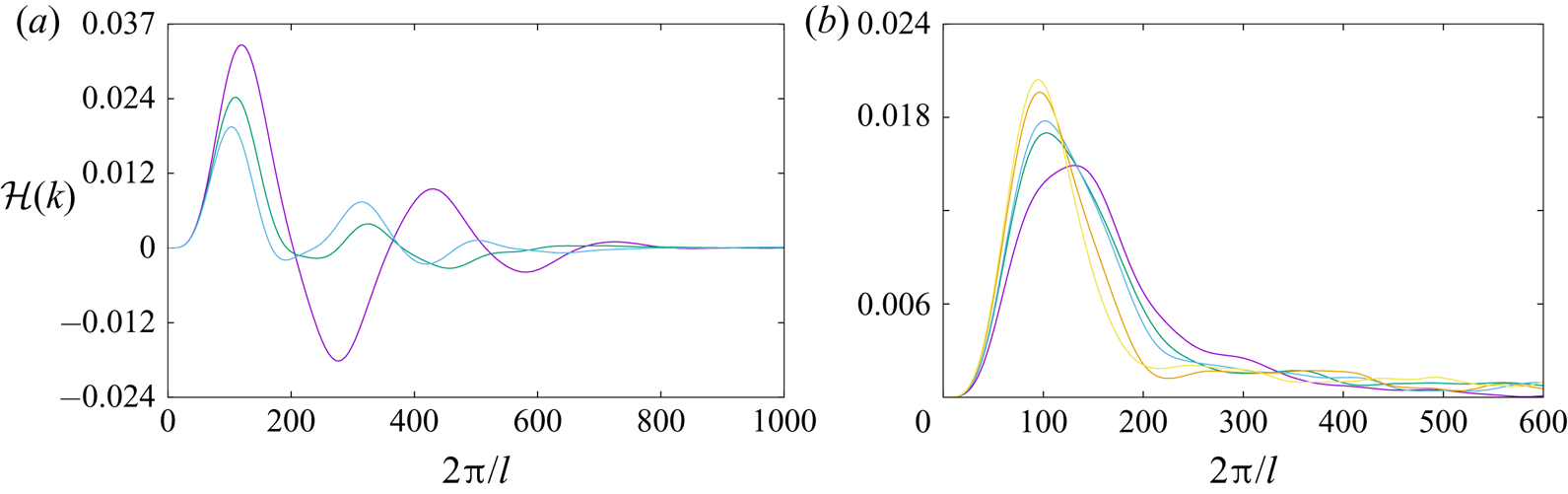
Figure 4. Vortex dynamics calculation. (a) Pre-reconnection helicity spectra  $\hat {\mathcal {H}}(k)$ at times $t=0$, $t=0.2$ and $t=0.28$ ( $t_u$ units). Smaller times correspond to curves with higher peaks at small wavenumbers. (b) Post-reconnection helicity spectra $\hat {\mathcal {H}}(k)$ at times $t=1.02$, $t=1.845$, $t=2.02$, $t=2.50$ and $t=2.825$ ( $t_u$ units). Larger times correspond to curves with higher peaks at smaller wavenumbers. As a result of an inverse helicity cascade, a peak is formed at small wavenumbers.
The above considerations suggest the usefulness of helicity spectra in characterizing vortex-dynamical processes. On the other hand, we have checked that the observed rapid changes in the topological measures of helicity do not affect the shape of the spectrum. This is understood by considering that helicity is a flow quantity that requires significant global changes in flow patterns in order to have its spectrum altered. On the other hand, the topology can change on a much faster scale in a ‘quantum’ fashion. As indicated by the results, it is reasonable to expect that different topologies could correspond to the same spectra. In other words, although helicity is always indicative of the amount of handedness in the flow, and therefore of the linking topology, we cannot use the latter to characterize key flow processes as the above inverse cascade. For this purpose, more potent topological measures would be needed, as are, for example, the above mentioned knot polynomials and Vassiliev invariants above the lowest order.
5.2. Navier–Stokes calculation
Computational complexity forbids probing high-Reynolds-number flows with Navier–Stokes calculations. Overcoming this limitation was a key motive for developing the vortex-dynamical approach. In this respect, a  $512^3$ grid size was shown to provide adequate resolution for capturing vortex link dynamics at $Re=1500$, where $Re=\varGamma /\nu$, $\varGamma$ (which is analogous to $\varGamma _m$ in the vortex-dynamical formulation) is the circulation of each vortex tube and $\nu$ is the viscosity of the fluid. The numerical method is a projection, finite-volume technique which is described in detail elsewhere (Kivotides Reference Kivotides2018b). The boundary conditions are periodic. To ensure that viscous dissipation processes are adequately captured, the calculation resolves their characteristic time scale $t_u=R_t^2/\nu$, where $R_t$ is the tube-core radius, which is equal to $0.2 R_c$, and $R_c$ is the tube-centreline radius. Time is scaled with $t_u$, total helicity $\mathcal {H} = \int _{\mathcal {V}} \boldsymbol {u}(\boldsymbol {x}) \boldsymbol {\cdot } \boldsymbol {\omega }(\boldsymbol {x})\,\textrm {d}\boldsymbol {x}$ with $\varGamma ^2$, mean enstrophy $\varOmega = (0.5/{\mathcal {V}}) \int _{\mathcal {V}} \boldsymbol {\omega }(\boldsymbol {x}) \boldsymbol {\cdot } \boldsymbol {\omega }(\boldsymbol {x})\,\textrm {d} \boldsymbol {x}$ with $t_u^{-2}$ and mean energy $\mathcal {E} = (0.5/{\mathcal {V}}) \int _{\mathcal {V}} \boldsymbol {u}(\boldsymbol {x}) \boldsymbol {\cdot } \boldsymbol {u}(\boldsymbol {x})\,\textrm {d}\boldsymbol {x}$ with $\varGamma \nu /R_c^2$. Notably, we show the total helicity (rather than the mean value as with energy and enstrophy), because the normalized $\mathcal {H}$ is equal to $2$, and we can directly compare with the vortex-dynamical results.
Due to the dissipative nature of the flow, there is monotonic energy decay (figure 5a). Similar to the vortex-dynamical case, Biot–Savart interactions induce a stretched structure of antiparallel vortices (figure 6a–d). This process intensifies enstrophy (figure 5b), and sustains energy and helicity dissipation rates (figure 5a,c). At time  $t=0.186$ (figure 6e), the system has proceeded beyond the enstrophy maximum; hence, the stretching process has concluded and the antiparallel vortex tubes comprising the stretched structure are in the process of annihilating each other via viscous diffusion. By time $t=29$ (figure 6f), the original link has disappeared, yet, despite the unlinking process, the system retains $70\,\%$ of its initial helicity (figure 5c). This is because there is now a significant amount of $Tw$ and $Wr$ in the system. Indeed, there is evidence of core torsion at the chosen isosurface level of $\vert \boldsymbol {\omega }\vert =154.4$ (figure 6e). Overall, there is agreement with the inviscid, vortex-dynamics results on $Lk$ transformation into other topological helicity measures. The Navier–Stokes calculation brings forward the merits of the vortex-dynamical approach, since it is tube discretization into elementary vortices, which are tracked in time, that enables the unambiguous computation of topological helicity measures in that case.
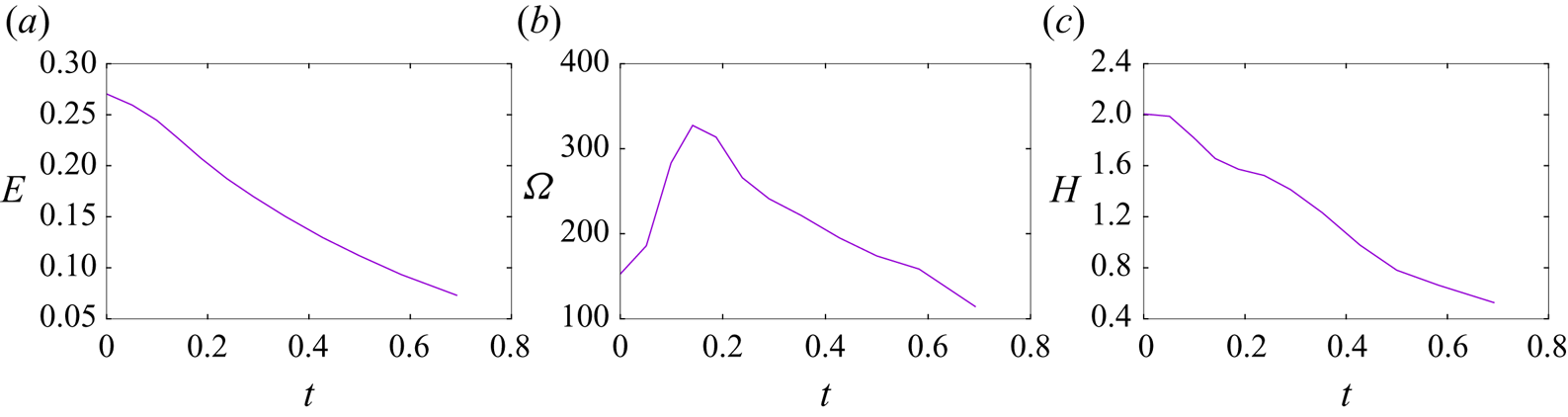
Figure 5. Navier–Stokes calculation. Vortex link at  $Re=1500$. (a) Scaled mean energy versus scaled time. (b) Scaled mean enstrophy versus scaled time. (c) Scaled total helicity versus scaled time.
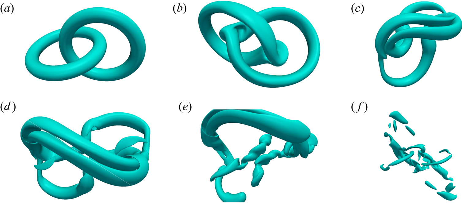
Figure 6. Vorticity magnitude isosurfaces at level  $\vert \boldsymbol {\omega }\vert =154.4$. From $(a)$ to $(f)$ the times are: $0$,
$0$,  $0.05$, $0.1$, $0.14$, $0.186$ and $0.29$.
Due to computational complexity of the Navier–Stokes  $\hat {\mathcal {H}}(k)$ formula, we present lower-resolution ( $64^3$) spectra (figure 7). Based on the expected inverse helicity cascade, this is not a true limitation. Since the Reynolds number is not very large, some effects of viscous dissipation on helicity physics are anticipated. The initial stages resemble the vortex-dynamical case (figure 7a). The spectral fluctuations are damped out, whilst the total helicity does not vary significantly. Similar to the inviscid case, there is a transition from alternating-sign helicity at different scales to exclusively positive values. At larger times (figure 7b), the inverse cascade of the inviscid case is present in an incomplete way. Indeed, there is a shift of spectral peaks towards low wavenumbers, but since helicity is not conserved, and in contrast with the vortex-dynamics case, the peak levels are decaying instead of increasing. Hence, it was the inviscid nature of our vortex-dynamical system that enabled the unambiguous demonstration of the inverse helicity cascade. This was achieved with a low computational complexity calculation, that required significantly smaller processing and memory capacities than the Navier–Stokes computation.
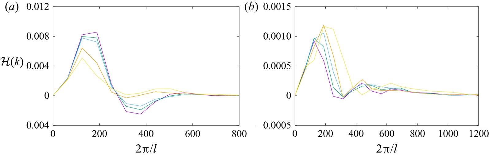
Figure 7. Navier–Stokes calculation. (a) Pre-enstrophy peak helicity spectra  $\hat {\mathcal {H}}(k)$ at times $t=0$, $t=0.025$, $t=0.037$, $t=0.075$ and $t=0.1$ ( $t_u$ units). Smaller times correspond to curves with higher peaks at small wavenumbers. (b) Post-enstrophy peak helicity spectra $\hat {\mathcal {H}}(k)$ at times $t=0.302$, $t=0.523$, $t=0.586$, $t=0.636$ and $t=0.686$ ( $t_u$ units). Larger times correspond to curves with peaks at smaller wavenumbers.
6. Conclusion
Vortex links are destroyed by reconnections which are facilitated by viscous diffusion that allows vortex lines to slip past each other. A byproduct of this process is the dissipation of energy and helicity. The energy sink is equal to  $-\int _{\mathcal {V}} \epsilon _e \,\textrm {d}\boldsymbol {x}$, with $\epsilon _e=2 \nu S_{ij} S_{ij}$ which for an unbounded system becomes $\epsilon _e=\nu \boldsymbol {\omega } \boldsymbol {\cdot } \boldsymbol {\omega }$, whilst the helicity sink is $-\int _{\mathcal {V}} \epsilon _h\,\textrm {d}\boldsymbol {x}$, with $\epsilon _h=2 \nu \boldsymbol {\omega } \boldsymbol {\cdot } \boldsymbol {\nabla } \times \boldsymbol {\omega }$. Since, as discussed in § 1, the conservation of helicity involves the vector product of velocity with frozen in the flow vector fields, it is reasonable to associate helicity dissipation with the diffusion of the same vector fields (here the vorticity) enabled by viscosity (Layton Reference Layton2007). Notably, the sink of streamline helicity is the vortex-line helicity (times $\nu$ for dimensional book-keeping). During reconnection, vortices are stretched, so both enstrophy and $\epsilon _e$ are intensified. The helicity sink has a different structure, but it too leads to a reduction of helicity. Our research suggests that disconnecting the reconnection phenomenon from its underlying physical mechanism (e.g. viscous dissipation in classical fluids, quantum stress action in quantum fluids or scissors and glue in Christmas ribbons (Pfister & Gekelman Reference Pfister and Gekelman1990)) can help understand better the experiments of Scheeler et al. (Reference Scheeler, Kleckner, Proment, Kindlmann and Irvine2014). Indeed, the purely topological act of reconnection conserves helicity (even if it destroys $Lk$) (Pfister & Gekelman Reference Pfister and Gekelman1990). On the other hand, the physical means by which reconnection is achieved could destroy some helicity as a byproduct of their action, but this ought not obfuscate the helicity-preserving nature of topological change. For example, in the classical fluid dynamics case, the short duration of high-Reynolds-number reconnection means that topological change can be achieved with small helicity destruction (since viscous dissipation does not have sufficient time to effect a sizeable reduction). Our calculations support these conclusions in two different ways: (a) by constructing, via the vortex-dynamics model of non-dissipative reconnections, a direct vortex analogue of the purely topological case of Pfister & Gekelman (Reference Pfister and Gekelman1990), and indicating that helicity tends to be preserved in this case, and (b) by solving the Navier–Stokes equations for a smaller Reynolds number, demonstrating that viscous reduction of helicity is just a secondary side effect of the reconnection process, which conceals the fundamental helicity-preserving nature of topological reconnections. This concealment becomes more and more feeble as the Reynolds number increases, until, in our idealized vortex-dynamical computation, it becomes negligible as we reach the limit of purely topological change.
Our calculation indicates a transformation of pre-reconnection  $Lk$ to post-reconnection $Wr$. In this way, it is in full agreement with the experimental results of Scheeler et al. (Reference Scheeler, Kleckner, Proment, Kindlmann and Irvine2014). Interestingly, the constant pre-reconnection $Lk$ values correspond to significant helicity spectrum dynamics, which conserve (in the inviscid limit) topology whilst eliminating small-scale helicity. The inverse helicity cascade computed here differs from the direct helicity cascade reported in the statistics of homogeneous, isotropic turbulence (Biferale, Musacchio & Toschi Reference Biferale, Musacchio and Toschi2013). To understand this result better, we note that the computed helicity spectrum of a link composed of single line vortices shows (progressively decaying) fast, sign-changing variations at all scales. Similar in origin to energy spectrum ringing in vortex rings, these fluctuations are due to the potential flow around the line vortices, since they are eliminated at subcore length scales, when we replace lines with tubes. Similar helicity spectrum oscillations were observed for two perpendicular thin slabs of magnetic flux (Asgari-Targhi & Berger Reference Asgari-Targhi and Berger2009). The key observation here is that, at every finite-scale interval, there is only a small net amount of helicity, as compared with the actual fluctuation amplitude. This is because there is a gradual reduction of the amplitude as we move towards smaller scales. These remarkable small-scale variations in the spectrum are directly related to the perfect-circle geometry of line vortices, and they disappear once the rings are deformed by Biot–Savart effects on the route to reconnection. However, since helicity is conserved, and the small-scale helicity associated with the perfect-circle geometry is destroyed as the rings become non-circular, the small-scale helicity needs to be transferred to larger scales. More concisely, small-scale helicity is associated with perfect-circle geometry and very small vortex cores, and as the geometry is altered on the route to reconnection whilst global helicity is conserved, the only physically viable process is for helicity to accumulate at large scales. The post-reconnection inverse helicity cascade has possibly important implications for the structure of turbulence. Indeed, the magnification of $\boldsymbol {u} \boldsymbol {\cdot } \boldsymbol {\omega }$ at large scales implies the weakening of the Lamb force $\boldsymbol {u} \times \boldsymbol {\omega }$, which is responsible for the nonlinearity of turbulence and the turbulence cascade. Perhaps some turbulent coherent structures are the remnants of reconnection-induced destructions of linked vortex rings. Thus, the post-reconnection dynamics could be associated with the formation of turbulent coherent structures and the inhibition of the direct energy cascade.
This work could be continued along various directions. It would be interesting, for example, to investigate the topological and helicity dynamics of magnetohydrodynamic vortex links. Such studies would significantly expand previous vortex-dynamical magnetohydrodynamic investigations (Kivotides Reference Kivotides2018a, Reference Kivotides2019). Another important problem is the topological and helicity dynamics of vortex knots, and possible connections between topology and energy and helicity spectra there, in conjunction with advanced topological measures including knot polynomials (Liu & Ricca Reference Liu and Ricca2015; Cooper et al. Reference Cooper, Mesgarnezhad, Baggaley and Barenghi2019) and Vassiliev invariants.
Declaration of interests
The authors report no conflict of interest.


 Open access