


1. Introduction
Transport of passive and active scalars in multiphase turbulence is very important in many industrial processes and natural phenomena, from vaporization of atomized fuel jets (Gorokhovski & Herrmann Reference Gorokhovski and Herrmann2008; Ashgriz Reference Ashgriz2011; Gao et al. Reference Gao, Chen, Qiu, Ding and Xie2022; Boyd & Ling Reference Boyd and Ling2023) to rain formation and atmosphere–ocean heat/mass exchanges (Duguid & Stampfer Reference Duguid and Stampfer1971; Deike Reference Deike2022) or even to the uptake of nutrients and other biochemicals by cells in complex flows (Aksnes & Egge Reference Aksnes and Egge1991; Magar & Pedley Reference Magar and Pedley2005). While the mixing of active or passive scalars in turbulent single-phase flows has been extensively analysed using experiments and simulations (Kim & Moin Reference Kim and Moin1989; Kasagi, Tomita & Kuroda Reference Kasagi, Tomita and Kuroda1992; Antonia & Orlandi Reference Antonia and Orlandi2003; Pirozzoli, Bernardini & Orlandi Reference Pirozzoli, Bernardini and Orlandi2016; Zonta, Marchioli & Soldati Reference Zonta, Marchioli and Soldati2012a; Zonta, Onorato & Soldati Reference Zonta, Onorato and Soldati2012b; Zonta & Soldati Reference Zonta and Soldati2014), when multiphase flows are considered, the situation becomes much more challenging (Gauding et al. Reference Gauding, Thiesset, Varea and Danaila2022; Ni Reference Ni2024).
One crucial aspect of multiphase turbulence – which makes the analysis of these flows particularly difficult – is the presence of interfaces that dynamically move and deform in time and space according to the flow conditions and that clearly alter/mediate heat and species transport and mixing, as well as phase change phenomena (Deckwer Reference Deckwer1980; Gvozdić et al. Reference Gvozdić, Alméras, Mathai, Zhu, van Gils, Verzicco, Huisman, Sun and Lohse2018; Liu et al. Reference Liu, Chong, Yang, Verzicco and Lohse2022; Pelusi et al. Reference Pelusi, Ascione, Sbragaglia and Bernaschi2023; Roccon, Zonta & Soldati Reference Roccon, Zonta and Soldati2023).
In this context, previous works mostly focused on the heat/mass transfer from/to isolated drops and bubbles using analytical (Boussinesq Reference Boussinesq1905; Levich Reference Levich1962; Bird, Stewart & Lightfoot Reference Bird, Stewart and Lightfoot2002), numerical (Bothe et al. Reference Bothe, Koebe, Wielage, Prüss and Warnecke2004; Figueroa-Espinoza & Legendre Reference Figueroa-Espinoza and Legendre2010; Herlina & Wissink Reference Herlina and Wissink2016; Albernaz et al. Reference Albernaz, Do-Quang, Hermanson and Amberg2017; Farsoiya, Popinet & Deike Reference Farsoiya, Popinet and Deike2021; Farsoiya et al. Reference Farsoiya, Magdelaine, Antkowiak, Popinet and Deike2023) and experimental techniques (Ohta, Shimoyama & Ohigashi Reference Ohta, Shimoyama and Ohigashi1975; Hiromitsu & Kawaguchi Reference Hiromitsu and Kawaguchi1995; Wu et al. Reference Wu, Hsu, Kuo and Sheen2003; Birouk & Gökalp Reference Birouk and Gökalp2006; Marti et al. Reference Marti, Martinez, Mazo, Garman and Dunn-Rankin2017). When swarms of drops/bubbles are considered, the number of available investigations is more limited. For very small drops/bubbles, numerical investigations usually rely on the Lagrangian approach, in which drops/bubbles are assumed to have sub-Kolmogorov size and are treated as material points (Kuerten Reference Kuerten2016; Maxey Reference Maxey2017; Chong et al. Reference Chong, Ng, Hori, Yang, Verzicco and Lohse2021; Wang et al. Reference Wang, Alipour, Soligo, Roccon, De Paoli, Picano and Soldati2021a; Wang, Dalla Barba & Picano Reference Wang, Dalla Barba and Picano2021b). When larger drops/bubbles are considered (i.e. larger than the Kolmogorov scale), the problem becomes more complex, since the interface shape and deformation play a crucial role. Not surprisingly, remarkable works in this context have appeared only recently, both for the case of passive scalar transport and for the case of active scalars/phase change (Méès et al. Reference Méès, Grosjean, Marié and Fournier2020; Dodd et al. Reference Dodd, Mohaddes, Ferrante and Ihme2021; Scapin et al. Reference Scapin, Dalla Barba, Lupo, Rosti, Duwig and Brandt2022; Shao, Jin & Luo Reference Shao, Jin and Luo2022; Hidman et al. Reference Hidman, Ström, Sasic and Sardina2023). Relevant to the present work is the observation done by Dodd et al. (Reference Dodd, Mohaddes, Ferrante and Ihme2021) and Scapin et al. (Reference Scapin, Dalla Barba, Lupo, Rosti, Duwig and Brandt2022), and also confirmed by the experiments of Méès et al. (Reference Méès, Grosjean, Marié and Fournier2020), where the Sherwood number (i.e. dimensionless mass transfer coefficient) measured during drop evaporation in turbulence is larger compared to that obtained from widely used correlations (Frössling Reference Frössling1938; Ranz Reference Ranz1952; Birouk & Gökalp Reference Birouk and Gökalp2002).
In this work, we focus on the numerical simulation of the heat transfer process in a drop-laden turbulent channel flow, particularly on the role of the Prandtl number  $Pr$, i.e. the ratio between momentum and thermal diffusivity, in the process. Compared with single-phase turbulence, where the range of scales that must be resolved to perform a direct numerical simulation (DNS) is purely dictated by the smallest scales of turbulence (Kolmogorov scale), when the mixing of scalars in multiphase turbulence is analysed, two further additional scales come into the picture. The first one is the Batchelor scale (Batchelor Reference Batchelor1959; Batchelor, Howells & Townsend Reference Batchelor, Howells and Townsend1959), which determines the smallest scale of the temperature/concentration field. The second important scale is the Kolmogorov–Hinze scale (Kolmogorov Reference Kolmogorov1941; Hinze Reference Hinze1955), and is linked to the multiphase nature of the flow. This scale can be used, perhaps with some limitations (Qi et al. Reference Qi, Tan, Corbitt, Urbanik, Salibindla and Ni2022), to determine the critical size of a drop/bubble that will not undergo breakage in turbulence. These two scales – and their corresponding ratio to the Kolmogorov scale, i.e. the smallest length scale of the turbulent flow field – control the system dynamics and define the minimal grid requirements that must be satisfied to perform a DNS of scalar mixing in multiphase turbulence (always keeping in mind that performing a simulation that resolves the interface dynamics down to the molecular scale is, at present, almost unfeasible). In this context, the major constraint is usually posed by the Batchelor scale, which becomes smaller than the Kolmogorov length scale when Prandtl numbers larger than unity are considered. Overall, the wide range of scales involved in the process makes simulations of scalar mixing in multiphase turbulence a challenging task and limits the space parameters that can be explored by means of DNS. Our simulations are initialized by injecting a swarm of large and deformable drops (initially warmer) inside a turbulent channel flow (initially colder). The system is described by coupling the DNS of turbulent heat transfer with a phase-field method, employed to describe the drop topology (Zheng et al. Reference Zheng, Babaee, Dong, Chryssostomidis and Karniadakis2015; Mirjalili, Jain & Mani Reference Mirjalili, Jain and Mani2022). We simulate realistic values of the Prandtl number up to $Pr=8$, similar to those obtained in liquid–liquid systems. We remark here that simulations of mass transfer problems in wall-bounded flow configurations, where the typical Schmidt number $Sc$ (i.e. the mass transfer counterpart of $Pr$) is ${O}({10^2 \sim 10^3})$, e.g. $Sc \simeq 600$ for $CO_2$ in freshwater (Wanninkhof Reference Wanninkhof1992), are currently out of reach even using the most advanced computing. Indeed, the resulting Batchelor scale would be at least one order of magnitude smaller, thus requiring grid resolutions comparable to or larger than those employed for state-of-the-art single-phase DNS (Lee & Moser Reference Lee and Moser2015; Pirozzoli et al. Reference Pirozzoli, Romero, Fatica, Verzicco and Orlandi2021) but with a much larger computational cost as the systems of equations to be solved are more complex and restrictive (also from the temporal discretization point of view).
The present study has three main objectives. First, we want to investigate the macroscopic dynamic of the drops and of the heat transfer process by analysing the drop size distribution and the mean temperature behaviour of the two phases over time. Second, we want to characterize the influence of the Prandtl number, i.e. of the microscopic flow properties, on the macroscopic flow properties (mean temperature, heat transfer coefficient) and, building on top of the numerical results, we want to develop a physical-based model to explain the observed results. Third, we want to study the influence of the Prandtl number and drop size on the temperature distribution inside the drops, so as to evaluate the corresponding flow mixing/ homogenization.
The paper is organized as follows. In § 2, the governing equations, the numerical method and the simulation setup are presented. In § 3, the simulation results, in terms of drop size distribution and mean temperature of the two phases and heat transfer coefficient, are carefully characterized and discussed. A simplified model is also developed to explain the observed results. The temperature distribution inside the drops is then evaluated at different Prandtl numbers and drop sizes. Finally, conclusions are presented in § 4.
2. Methodology
We consider a swarm of large and deformable drops injected in a turbulent channel flow. The channel has dimensions  $L_x \times L_y \times L_z = 4 {\rm \pi}h \times 2 {\rm \pi}h \times 2h$ along the streamwise ( $x$), spanwise ( $\kern 0.06em y$) and wall-normal direction ( $z$). To describe the dynamics of the system, we couple DNS of the Navier–Stokes and energy equations, used to describe the turbulent flow, with a phase-field method (PFM), used to describe the interfacial phenomena. The employed numerical framework is described in more detail in the following.
2.1. Phase-field method
To describe the dynamics of drops and the corresponding topological changes (e.g. coalescence and breakage), we employ an energy-based PFM (Jacqmin Reference Jacqmin1999; Badalassi, Ceniceros & Banerjee Reference Badalassi, Ceniceros and Banerjee2003; Roccon et al. Reference Roccon, Zonta and Soldati2023), which is based on the introduction of a scalar quantity, the phase field  $\phi$, required to identify the two phases. The phase field $\phi$ has a uniform value in the bulk of each phase ( $\phi =+1$ inside the drops; $\phi =-1$ inside the carrier fluid) and undergoes a smooth change across the thin transition layer that separates the two phases. The transport of the phase field variable is described by a Cahn–Hilliard equation, which in dimensionless form reads as
 \begin{equation} \frac{\partial \phi}{\partial t} + {\boldsymbol u} \boldsymbol{\cdot} \boldsymbol{\nabla} \phi = \frac{1}{Pe} \nabla^2 \mu_\phi + f_p , \end{equation}
where  ${\boldsymbol u}=(u,v,w)$ is the velocity vector, $Pe$ is the Péclet number, $\mu$ is the phase field chemical potential and $f_p$ is a penalty-flux term which will be further discussed later. The Péclet number is
 \begin{equation} Pe=\frac{u_\tau^* h^* }{{\mathcal{M}^*} \beta^*}, \end{equation}
where  $u^*_\tau$ is the friction velocity ( $u_\tau ^*=\sqrt {\tau _w^*/\rho ^*}$, with $\tau _w^*$ the wall-shear stress and $\rho ^*=\rho _c^*=\rho _d^*$ the density of the fluids), $h^*$ is the channel half-height, ${\mathcal {M}}^*$ is the mobility and $\beta ^*$ is a positive constant (the superscript $^*$ is used to denote dimensional quantities hereinafter). The chemical potential $\mu$ is defined as the variational derivative of a Ginzburg–Landau free-energy functional, the expression of which is chosen to represent an immiscible binary mixture of fluids (Soligo, Roccon & Soldati Reference Soligo, Roccon and Soldati2019a,Reference Soligo, Roccon and Soldatib,Reference Soligo, Roccon and Soldatic). The functional is the sum of two contributions: the first contribution, $f_0$, accounts for the tendency of the system to separate into the two pure stable phases, while the second contribution, $f_{mix}$, is a mixing term accounting for the energy stored at the interface (i.e. surface tension). The mathematical expression of the functional in dimensionless form is
 \begin{equation} \mathcal{F}[\phi, \boldsymbol{\nabla} \phi]= {\int_{\varOmega} \left( \underbrace{\frac{({\phi}^2-1)^2}{4}}_{f_0}+\underbrace{\frac{Ch^2}{2} | \boldsymbol{\nabla} \phi |^2}_{f_{mix}} \right)} \mathrm{d} \varOmega , \end{equation}
where  $\varOmega$ is the considered domain and $Ch$ is the Cahn number, which represents the dimensionless thickness of the thin interfacial layer between the two fluids:
 \begin{equation} Ch=\frac{\xi^*}{h^*} , \end{equation}
where  $\xi ^*$ is clearly the dimensional thickness of the interfacial layer. From (2.3), the expression of the chemical potential can be derived as the functional derivative with respect to the order parameter:
 \begin{equation} \mu_\phi=\frac{\delta \mathcal{F}[\phi \boldsymbol{\nabla} \phi ]}{\delta \phi}={\phi}^3 - \phi - Ch^2 \nabla^2 \phi . \end{equation}
At equilibrium, the chemical potential is constant throughout all the domain. The equilibrium profile for a flat interface can thus be obtained by solving  $\boldsymbol {\nabla } \mu _\phi = \boldsymbol {0}$, hence,
 \begin{equation} \phi_{eq}=\tanh \left( \frac{s}{\sqrt{2}Ch}\right), \end{equation}
where  $s$ is the coordinate normal to the interface. As anticipated before, the last term in the right-hand side of the Cahn–Hilliard equation (2.1) is a penalty-flux term employed in the profile-corrected formulation of the PFM, and is used to overcome some potential drawbacks of the standard formulation of the method, e.g. mass leakages among the phases and misrepresentation of the interfacial profile (Yue, Zhou & Feng Reference Yue, Zhou and Feng2007; Li, Choi & Kim Reference Li, Choi and Kim2016). This penalty flux is defined as
 \begin{equation} f_p=\frac{\lambda}{Pe} \left[ \nabla^2 \phi -\frac{1}{\sqrt{2}Ch} \boldsymbol{\nabla} \boldsymbol{\cdot} \left( (1-{\phi}^2) \frac{\boldsymbol{\nabla}\phi}{|\boldsymbol{\nabla}\phi|} \right) \right] , \end{equation}
where  $\lambda =0.0625/Ch$ (Soligo et al. Reference Soligo, Roccon and Soldati2019c).
2.2. Hydrodynamics
To describe the hydrodynamics of the multiphase system, the Cahn–Hilliard equation is coupled with the Navier–Stokes equations. The presence of a deformable interface (and of the corresponding surface tension forces) is accounted for by introducing an interfacial term in the Navier–Stokes equations. Recalling that in the present case, we consider two fluids with the same density ( $\rho ^*=\rho _c^*=\rho _d^*$) and viscosity ( $\mu ^*=\mu _c^* =\mu _d^*$), the continuity and Navier–Stokes equations in dimensionless form read as
 \begin{gather} \boldsymbol{\nabla} \boldsymbol{\cdot} \boldsymbol{u}=0 , \end{gather}
 \begin{gather}\frac{\partial \boldsymbol{u}}{\partial t}+\boldsymbol{u} \boldsymbol{\cdot} \boldsymbol{\nabla} \boldsymbol{u} ={-}\boldsymbol{\nabla} p +\frac{1}{Re_\tau} \nabla^2 \boldsymbol{u} + \frac{3}{\sqrt{8}}\frac{Ch}{We} \boldsymbol{\nabla} \boldsymbol{\cdot} \boldsymbol{T_c}. \end{gather}
Here  $p$ is the pressure field, while $\boldsymbol {T_c}$ is the Korteweg tensor (Korteweg Reference Korteweg1901) used to account for the surface tension forces and defined as
 \begin{equation} \boldsymbol{T_c}=|\boldsymbol{\nabla}\phi |^2 \boldsymbol{I}-\boldsymbol{\nabla}\phi \otimes \boldsymbol{\nabla} \phi , \end{equation}
where  $\boldsymbol I$ is the identity matrix and $\otimes$ represents the dyadic product. This approach is the continuum surface stress approach (Lafaurie et al. Reference Lafaurie, Nardone, Scardovelli, Zaleski and Zanetti1994; Gueyffier et al. Reference Gueyffier, Li, Nadim, Scardovelli and Zaleski1999) applied in the context of the PFM, and is analytically equivalent to the chemical potential forcing (Mirjalili, Khanwale & Mani Reference Mirjalili, Khanwale and Mani2023). The dimensionless groups appearing in the Navier–Stokes equations are the shear Reynolds number $Re_\tau$ (ratio between inertial and viscous forces) and the Weber number $We$ (ratio between inertial and surface tension forces), which are defined as
 \begin{equation} Re_\tau=\frac{\rho^* u_\tau^* h^*}{\mu^*}, \quad We=\frac{\rho^* {{u_\tau^*}}^2 h^*}{\sigma^*},\end{equation}
where  $\sigma ^*$ is the surface tension. Note that, consistently with the employed adimensionalization, $We$ is defined using the half-channel height (and not the drop diameter).
2.3. Energy equation
The time evolution of the temperature field is obtained by solving the energy equation using a one-scalar model approach (Zheng et al. Reference Zheng, Babaee, Dong, Chryssostomidis and Karniadakis2015). To avoid the introduction of further complexity in the system, we consider two fluids with the same thermophysical properties, i.e. same thermal conductivity  $\lambda ^*$, same specific heat capacity $c_p^*$ and therefore same thermal diffusivity $a^*=\lambda ^*/\rho ^* c_p^*$ (since the density of the two phases is also the same). These properties have been evaluated at a reference temperature $\theta _{r}^*=(\theta _{d,0}^* + \theta _{c,0}^*)/2$, i.e. the average between the initial drop temperature and the carrier fluid temperature, and are assumed to be constant and uniform. Within these assumptions, the energy equation written in dimensionless form reads as
 \begin{equation} \frac{\partial \theta }{\partial t} + {\boldsymbol u} \boldsymbol{\cdot} \boldsymbol{\nabla} \theta = \frac{1}{Re_\tau Pr} \nabla^2 \theta , \end{equation}
where  $Pr$ is the Prandtl number defined as
 \begin{equation} Pr=\frac{\mu^* c_p^*}{\lambda^*}=\frac{\nu^*}{a^*}, \end{equation}
with  $\nu ^*=\mu ^*/\rho ^*$ the kinematic viscosity (i.e. momentum diffusivity). From a physical viewpoint, $Pr$ represents the momentum-to-thermal diffusivity ratio.
2.4. Numerical discretization
The governing equations (2.1), (2.8), (2.9) and (2.12) are solved using a pseudo-spectral method, which uses Fourier series along the periodic directions (streamwise and spanwise) and Chebyshev polynomials along the wall-normal direction. The Navier–Stokes and continuity equations are solved using a wall-normal velocity-vorticity formulation: (2.9) is rewritten as a fourth-order equation for the wall-normal component of the velocity  $w$ and a second-order equation for the wall-normal component of the vorticity $\omega _z$ (Kim, Moin & Moser Reference Kim, Moin and Moser1987; Speziale Reference Speziale1987). The Cahn–Hilliard equation (2.1), which in its original form is a fourth-order equation and is split into two second-order equations using the splitting scheme proposed by Badalassi et al. (Reference Badalassi, Ceniceros and Banerjee2003). Using this scheme, the governing equations are recasted as a coupled system of Helmholtz equations, which can be readily solved.
The governing equations are time-advanced using an implicit-explicit scheme. For the Navier–Stokes, the linear part is integrated using a Crank–Nicolson implicit scheme, while the nonlinear part is integrated using an Adams–Bashforth explicit scheme. Similarly, for the Cahn–Hilliard and energy equations, the linear terms are integrated using an implicit Euler scheme, while the nonlinear terms are integrated in time using an Adams–Bashforth scheme. The adoption of the implicit Euler scheme for the Cahn–Hilliard equation helps to damp unphysical high-frequency oscillations that could arise from the steep gradients of the phase field.
As the characteristic length scales of the flow and temperature fields, represented by the Kolmogorov scale,  $\eta _k^+$, and the Batchelor scale, $\eta _\theta ^+$, are different when non-unitary Prandtl numbers are employed (being these two quantities linked by the following relation $\eta _\theta ^+=\eta _k^+/\sqrt {Pr}$), a dual grid approach is employed to reduce the computational cost of the simulations and, at the same time, to fulfil the DNS requirements. In particular, when super-unitary Prandtl numbers are simulated, a finer grid is used to resolve the energy equation. Spectral interpolation is used to upscale/downscale the fields from the coarse to the refined grid and vice versa when required (e.g. upscaling of the velocity field to compute the advection terms in the energy equation).
This numerical scheme has been implemented in a parallel Fortran 2003 MPI in-house proprietary code. The parallelization strategy is based on a 2-D domain decomposition to divide the workload among all the MPI tasks. The solver execution is accelerated using openACC directives and CUDA Fortran instructions (solver execution) while the Nvidia cuFFT libraries are used to accelerate the execution of the Fourier/Chebyshev transforms. Overall, the computational method adopted allows for the accurate resolution of all the governing equations and the achievement of an excellent parallel efficiency thanks to the fine-grain parallelism offered by the numerical method used. The equivalent computational cost of the simulations is approximately 25 million CPU hours and the resulting dataset has a size of approximately 16 TB.
2.5. Boundary conditions
The system of governing equations is complemented by a set of suitable boundary conditions. For the Navier–Stokes equations, no-slip boundary conditions are enforced at the top and bottom walls (located at  $z=\pm h$):
 \begin{equation} {\boldsymbol u} (z={\pm} h)=\boldsymbol{0} . \end{equation}
For the Cahn–Hilliard equation, no-flux boundary conditions are applied at the two walls, yielding to the following boundary conditions:
 \begin{equation} \frac{\partial \phi}{\partial z}(z={\pm} h)=0 ; \quad \frac{\partial^3 \phi}{\partial {z}^3}(z={\pm} h)=0 . \end{equation}
Likewise, for the energy equation, no-flux boundary conditions are applied at the two walls (i.e. adiabatic walls):
 \begin{equation} \frac{\partial \theta}{\partial z}(z={\pm} h)=0 . \end{equation}
 Along the streamwise and spanwise directions ( $x$ and $y$), periodic boundary conditions are imposed for all variables (Fourier discretization). The adoption of these boundary conditions leads to the conservation of the phase field and temperature fields over time:
 \begin{equation} \frac{\partial}{\partial t} \int_{\varOmega} \phi \,\mathrm{d} \varOmega = 0 ; \quad \frac{\partial}{\partial t} \int_{\varOmega} \theta \,\mathrm{d} \varOmega = 0,\end{equation}
where  $\varOmega$ is the computational domain. Regarding the phase-field, (2.17a,b) enforces mass conservation of the entire system but does not guarantee the conservation of the mass of each phase (Yue et al. Reference Yue, Zhou and Feng2007; Soligo et al. Reference Soligo, Roccon and Soldati2019c), as some leakages between the phases may occur. This drawback is rooted in the PFM and more specifically in the curvature-driven flux produced by the chemical potential gradients (Kwakkel, Fernandino & Dorao Reference Kwakkel, Fernandino and Dorao2020; Mirjalili & Mani Reference Mirjalili and Mani2021). This issue is successfully mitigated with the adoption of the profile-corrected formulation that largely reduces this phenomenon. In the present cases, mass leakage between the phases occurs only in the initial transient when the phase field is initialized (see the section below for details on the initial condition) and is limited to 2 % of the initial mass of the drops. After this initial transient, the mass of each phase remains constant.
2.6. Simulation set-up
The turbulent channel flow, driven by an imposed constant pressure gradient in the streamwise direction, has a shear Reynolds number  $Re_\tau =300$. The computational domain has dimensions $L_x \times L_y \times L_z= 4{\rm \pi} h \times 2{\rm \pi} h \times 2h$, which corresponds to $L_x^+ \times L_y^+ \times L_z^+=3770 \times 1885 \times 600$ wall units. The value of the Weber number is kept constant and is equal to $We=3.00$, so to be representative of liquid/liquid mixtures (Than et al. Reference Than, Preziosi, Joseph and Arney1988). To study the influence of the Prandtl number $Pr$ on the heat transfer process, we consider four different values of $Pr$:
$Pr$:  $Pr=1$, $Pr=2$, $Pr=4$ and $Pr=8$. These values cover a wide range of real-case scenarios: from low-Prandtl-number fluids to water–toluene mixtures.
The grid resolution used to resolve the continuity, Navier–Stokes and Cahn–Hilliard equations is equal to  $N_x \times N_y \times N_z = 1024 \times 512 \times 513$ for all the cases considered in this work. For the energy equation, the same grid used for the flow field and phase field is employed at the lower Prandtl numbers ( $Pr=1$ and $Pr=2$), while a more refined grid, with $N_x \times N_y \times N_z = 2048 \times 1024 \times 513$ points, is used when the larger Prandtl numbers are considered ( $Pr=4$ and $Pr=8$). The computational grid has uniform spacing in the homogeneous directions, while Chebyshev–Gauss–Lobatto points are used in the wall-normal direction. We refer the reader to table 1 for an overview of the main physical and computational parameters of the simulation. For the employed grid resolution, the Cahn number is set to $Ch = 0.01$ while, to achieve convergence to the sharp interface limit, the corresponding phase field Péclet number is $Pe = 1/Ch = 50$.
Table 1. Overview of the simulation parameters. For a fixed shear Reynolds number  $Re_\tau =300$ and Weber number $We=3$, we consider a single-phase flow case and four non-isothermal drop-laden flows characterized by different Prandtl numbers: from $Pr=1$ to $Pr=8$. The grid resolution is modified accordingly so as to satisfy DNS requirements.

All simulations are initialized by releasing a regular array of 256 spherical drops with diameter  $d = 0.4h$ (corresponding to $d^+ = 120 w.u.$) inside a fully developed turbulent flow field (obtained from a preliminary simulation). To ensure the independence of the results from the initial flow field condition, each case is initialized with a slightly different flow field realization. Naturally, the fields are equivalent in terms of statistics as they are all obtained from a statistically steady turbulent channel flow. The volume fraction of the drops is $\varPhi = V_d/(V_c + V_d) = 5.4\,\%$, with $V_d$ and $V_c$ the volume of the drops and carrier fluid, respectively.
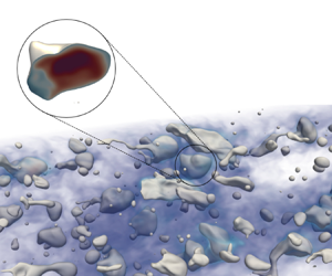
The initial condition for the temperature field is such that all drops are initially warm (initial temperature  $\theta _{d,0}=1$), while the carrier fluid is initially cold (initial temperature $\theta _{c,0}=0$). To avoid numerical instabilities that might arise from a discontinuous temperature field, the transition between drops and carrier fluid is initially smoothed using a hyperbolic tangent kernel. Figure 1 (which is an instantaneous snapshot captured at $t^+=1000$, for $Pr=1$) shows a volume rendering of the temperature field (blue, cold; red, hot), inside which deformable drops (whose interface, iso-level $\phi =0$, is shown in white) are transported.

Figure 1. Rendering of the computational setup employed for the simulations. A swarm of large and deformable drops is released in a turbulent channel flow. The temperature field is volume-rendered (blue, low; red, high) and the drop interface is shown in white (iso-level  $\phi =0$). Drops have a temperature higher than the carrier fluid (close-up view). The snapshot refers to $Pr=1$ and $t^+=1000$.
3. Results
Results obtained from the numerical simulations will be first discussed from a qualitative viewpoint, by looking at instantaneous flow and drop visualizations, and then analysed from a more quantitative viewpoint, by looking at the drop size distribution (DSD), and at the effect of the Prandtl number  $Pr$ on the average drops and fluid temperature. To explain the numerical results, and to offer a possible parametrization of the heat transfer process in drop-laden flows, we will also develop a simplified phenomenological model of the system. Finally, we will characterize the temperature distribution inside the drops, elucidating the effects of $Pr$ and of the drop size on it. Note that, unless differently mentioned, results are presented using the wall-unit scaling system but for the temperature field, which is made dimensionless using the initial temperature difference as a reference scale (which is a natural choice in the present case).
3.1. Qualitative discussion
The complex dynamics of drops immersed in a non-isothermal turbulent flow is visualized in figure 1, where the drops (identified by iso-contour of  $\phi =0$) are shown together with a volume-rendered distribution of temperature in the carrier fluid. Also shown in figure 1 is a close-up view of the temperature distribution inside the drop. We can notice that most of the drops – because of their deformability – gather at the channel centre, as also observed in previous studies in similar configurations (Scarbolo, Bianco & Soldati Reference Scarbolo, Bianco and Soldati2016; Soligo, Roccon & Soldati Reference Soligo, Roccon and Soldati2020; Mangani et al. Reference Mangani, Soligo, Roccon and Soldati2022).
Once injected into the flow, each drop starts interacting with the flow and with the neighbouring drops. The result of the drop–turbulence and drop–drop interactions is the occurrence of breakage and coalescence events. A breakage event happens when the flow vigorously stretches the drop, leading to the formation of a thin ligament that breaks and generates two child drops. Upon separation, surface tension forces tend to retract the broken filaments and restore the drop spherical shape. A coalescence event is observed when two drops come close to each other. The small liquid film that separates the drops starts to drain, and a coalescence bridge is formed. Later, surface tension forces enter the picture, reshaping the drop and completing the coalescence process. The dynamic competition between breakage and coalescence events, and their interaction with the turbulent flow, determines the number of drops, their size distribution, and their shape/morphology (i.e. curvature, interfacial area, etc.).
In the present case, drops not only exchange momentum with the flow and with the other drops but also heat. Starting from an initial condition characterized by warm drops (with uniform temperature) and cold carrier fluid, and because of the imposed adiabatic boundary conditions, the system evolves towards an equilibrium isothermal state. During the transient to attain this thermal equilibrium state, heat is transported by diffusion and advection inside each of the two phases, and across the interface of the drops (see the temperature field inside and outside the drops, figure 1). The picture is then further complicated by the occurrence of breakage and coalescence events. This is represented in figure 2. When breakage occurs (figure 2a–e), a thin filament is generated (figure 2a–c), which then leads to the formation of a smaller satellite drop (figure 2d,e). The filament and the satellite drop, given the large surface-to-volume ratio, exchange heat very efficiently and rapidly become colder. In contrast, when a coalescence occurs (figure 2f–o), two drops having different temperatures merge together. This induces an efficient mixing process, during which cold parcels of one drop become warmer and vice versa, warm parcels of the other drops become colder. Overall, breakup and coalescence events induce heat transfer modifications that are, in general, hard to predict a priori, since they do depend on the relative size of the involved parents/child drops.

Figure 2. Influence of topology changes on heat transfer: time sequence (a–e) of a breakage event and (f–o) of a coalescence event. During a breakage event, heat is transferred from the drops to carrier fluid thanks to the high surface/volume ratio of the pinch-off region. In the middle and bottom rows, the mixing between parcels of fluid with different temperatures can be appreciated. The two sequences refer to the case  $Pr=1$ and snapshots are separated by ${\rm \Delta} t^+ =15$. As a reference, the Kolmogorov–Hinze scale, $d^+_H$, is also reported.
Naturally, the problem of heat transfer in drop-laden turbulence is strongly influenced by the Prandtl number of the flow. This can be appreciated by looking at figure 3, where we show the instantaneous temperature field, together with the shape of the drops, at a certain instant in time ( $t^+=1500$) and at different Prandtl numbers: (a) $Pr=1$; (b) $Pr=2$; (c) $Pr=4$ and (d) $Pr=8$. In each panel, the temperature field is shown on a wall-parallel $x^+$- $y^+$ plane located at the channel centre ( $z^+=0$) and is visualized with a blue-red scale (blue, low; red, high). We observe that the temperature field changes significantly with $Pr$. In particular, we notice an increase in the drop-to-fluid temperature difference for increasing $Pr$, going from $Pr=1$ (figure 3a) where this difference is small, to $Pr=8$ (figure 3d) where this difference is large. The heat transfer from the drops to the carrier fluid becomes slower as $Pr$ increases, consistent with a physical situation in which the $Pr$ number is increased by reducing the thermal diffusivity of the fluid while keeping the momentum diffusivity constant (i.e. constant kinematic viscosity, and hence shear Reynolds number). Also, the temperature structures, both inside and outside the drop, become thinner and more complicated at higher $Pr$, since their characteristic length scale, the Batchelor scale $\eta _\theta ^+ \propto {Pr}^{-1/2}$, becomes smaller for increasing $Pr$ (Batchelor Reference Batchelor1959; Batchelor et al. Reference Batchelor, Howells and Townsend1959). In addition, smaller drops have, on average, a lower temperature compared to larger drops, regardless of the value of $Pr$. All these aspects will be discussed in more detail in the next sections.

Figure 3. Instantaneous visualization of the temperature field (red, hot; blue, cold) on a  $x^+-y^+$ plane located at the channel centre for $t^+=1500$. Drop interfaces (iso-level $\phi =0$) are reported using white lines. Each panel refers to a different Prandtl number. By increasing the Prandtl number (from top to bottom), the heat transfer becomes slower.
3.2. Drop size distribution
To characterize the collective dynamics of the drops, we compute the DSD at steady-state conditions, averaging over a time window  ${\rm \Delta} t^+=3000$, from $t^+=3000$ to $6000$. The achievement of steady-state conditions is here evaluated by monitoring global flow properties, like flow rate and wall stress, and drop properties, like the number of drops and the overall drop surface. It is worth mentioning that a quasi-equilibrium DSD, very close to the steady one, is already achieved at $t^+ \simeq 750$, and only minor changes occur to the DSD afterwards.
Figure 4 shows the DSD obtained for the different cases considered here:  $Pr=1$ (dark violet), $Pr=2$ (violet), $Pr=4$ (pink) and $Pr=8$ (light pink). Drop size distribution profiles are statistically the same. Small differences are due to the initial turbulence field, which is different for each simulation (see § 2.6). The DSDs have been computed considering, for each drop, the diameter of the equivalent sphere computed as
 \begin{equation} d_{eq}^+ = \left( \frac{6 V^+}{\rm \pi} \right)^{1/3}, \end{equation}
where  $V^+$ is the volume of the drop. Also reported in figure 4 is the Kolmogorov–Hinze scale, $d^+_H$, which can be computed as (Perlekar, Biferale & Sbragaglia Reference Perlekar, Biferale and Sbragaglia2012; Roccon et al. Reference Roccon, De Paoli, Zonta and Soldati2017; Soligo et al. Reference Soligo, Roccon and Soldati2019a)
 \begin{equation} d_H^+ = 0.725 \left(\frac{We}{Re_\tau} \right) ^{{-}3/5} | \epsilon_c|^{{-}2/5}, \end{equation}
where  $\epsilon _c$ is the turbulent dissipation, here evaluated at the channel centre where most of the drops collect because of their deformability (Lu & Tryggvason Reference Lu and Tryggvason2007; Soligo et al. Reference Soligo, Roccon and Soldati2020; Mangani et al. Reference Mangani, Soligo, Roccon and Soldati2022). Although recently challenged (Qi et al. Reference Qi, Tan, Corbitt, Urbanik, Salibindla and Ni2022; Vela-Martín & Avila Reference Vela-Martín and Avila2022; Ni Reference Ni2024), the Kolmogorov–Hinze scale (Kolmogorov Reference Kolmogorov1941; Hinze Reference Hinze1955) still represents a convenient estimate to evaluate the critical diameter below which drop breakage is unlikely to occur. Based on the Kolmogorov–Hinze scale, we can identify two different regimes (Garrett, Li & Farmer Reference Garrett, Li and Farmer2000; Deane & Stokes Reference Deane and Stokes2002; Deike Reference Deike2022). For drops smaller than the Kolmogorov–Hinze scale, we find the coalescence-dominated regime (left, grey area), in which drops that are smaller than the critical scale are generally not prone to break (although violent breakages can happen also for smaller drops). For drops larger than the Kolmogorov–Hinze scale, we find the breakage-dominated regime (right, white area) in which drop breakage is more likely to happen. Each regime is characterized by a specific scaling law, which describes the behaviour of the drop number density as a function of the drop size (Garrett et al. Reference Garrett, Li and Farmer2000; Deane & Stokes Reference Deane and Stokes2002; Chan, Johnson & Moin Reference Chan, Johnson and Moin2021): probability density function (PDF) $\sim {d_{eq}^+}^{-3/2}$ below Kolmogorov–Hinze scale and PDF $\sim {d_{eq}^+}^{-10/3}$ above it. The two scalings are represented by dot-dashed lines in figure 4.

Figure 4. Steady-state DSD obtained for:  $Pr=1$ (dark violet, circles), $Pr=2$ (violet, squares), $Pr=4$ (pink, diamonds) and $Pr=8$ (light pink, triangles). The Kolmogorov–Hinze (KH) scale $d^+_H$ is reported with a vertical dashed line while the two analytical scaling laws, ${d_{eq}^+}^{-3/2}$ for the coalescence-dominated regime (small drops, grey region) and ${d_{eq}^+}^{-10/3}$ for the breakage-dominated regime (larger drops, white region), are reported with dash-dotted lines.
We note that for equivalent diameters above the Hinze scale, our results follow quite well the theoretical scaling law and match the size distributions of the drops/bubbles obtained in the literature considering similar flow instances (Deike, Melville & Popinet Reference Deike, Melville and Popinet2016; Soligo, Roccon & Soldati Reference Soligo, Roccon and Soldati2021; Deike Reference Deike2022; Di Giorgio, Pirozzoli & Iafrati Reference Di Giorgio, Pirozzoli and Iafrati2022; Crialesi-Esposito, Chibbaro & Brandt Reference Crialesi-Esposito, Chibbaro and Brandt2023). Below the Hinze scale, for equivalent diameters in the range  $25<{d_{eq}^+}<{d_{H}^+}$, our results match reasonably well the theoretical scaling law. For equivalent diameters ${d_{eq}^+}<25~w.u.$, we observe an underestimation of the DSD compared with the proposed scaling. This is linked to the grid resolution, and in particular to the problem in describing very small drops (Soligo et al. Reference Soligo, Roccon and Soldati2021; Roccon et al. Reference Roccon, Zonta and Soldati2023).
3.3. Mean temperature of drops and carrier fluid
We now focus on the average temperature of the drops and of the carrier fluid. We consider the ensemble of all drops as one phase and the carrier fluid as the other phase (using the value of the phase field as a phase discriminator), and we compute the average temperature for each phase. The evolution in time of the drops and carrier fluid temperature,  ${\bar {\theta }}_d$ and ${\bar {\theta }}_c$, respectively, is shown in figure 5 for the different values of $Pr$. Together with the results obtained by current DNS, filled symbols in figure 5, we also show the predictions obtained by a simplified phenomenological model (solid lines), the details of which will be described and discussed later (see § 3.4). We start considering the DNS results only. As expected, we observe that the average temperature of the drops (violet to pink symbols) decreases in time, while the average temperature of the carrier fluid (blue to cyan symbols) increases in time, until the thermodynamic equilibrium, at which both phases have the same temperature, is asymptotically reached. For this reason, simulations have been run long enough for the average temperature of both phases to be sufficiently close to the equilibrium temperature. In particular, we stopped the simulations at $t^+ \simeq 6000$, when the condition
 \begin{equation} \frac{(\bar{\theta}_d - \theta_{eq})}{(\theta_{d,0} -\theta_{eq})} \leq 0.05, \end{equation}
with  $\theta _{d,0}$ the initial temperature of the drops, is satisfied by all simulations. The equilibrium temperature, $\theta _{eq}$, can be easily estimated a priori: since the two walls are adiabatic and the homogeneous directions are periodic, the energy of the system is conserved over time. After some algebra and recalling the definition of volume fraction, $\varPhi =V_d/(V_d+ V_c)$, we obtain the equilibrium temperature:
 \begin{equation} \theta_{eq}= \theta_{c,0}(1-\varPhi) + \theta_{d,0} \varPhi , \end{equation}
which is represented by the horizontal dashed line in figure 5.

Figure 5. Time evolution of the mean temperature of drops (violet to pink colours, different symbols) and carrier fluid (blue to cyan colours, different symbols) for the different Prandtl numbers considered. DNS results are reported with full circles while the predictions obtained from the model are reported with continuous lines. The equilibrium temperature of the system,  $\theta _{eq}$, is reported with a horizontal dashed line.
Figure 5 also provides a clear indication that a higher Prandtl number results in a longer time required for the system to reach the equilibrium temperature,  $\theta _{eq}$. The trend can be observed for both the drops and carrier fluid, as the two phases are mutually coupled (the heat released from the drops is adsorbed by the carrier fluid). This result confirms our previous qualitative observations, see figure 3 and discussion therein, where a large $Pr$ (small thermal diffusivity) reduces the heat released by the drops. It is also interesting to observe that the behaviour of the mean temperature of the two phases appears self-similar at the different $Pr$.
$Pr$.
3.4. A phenomenological model for heat transfer rates in droplet laden flows
In an effort to provide a possible interpretation of the previous results – and in particular to explain the average temperature behaviour shown in figure 5 – we develop a simple physically sound model of the heat transfer in drop-laden turbulence. We start by considering the heat transfer mechanisms from a single drop of diameter  $d^*$ to the surrounding fluid:
 \begin{equation} m^*_d c_p^* \frac{\partial \theta^*_d}{\partial t^*}= \mathcal{H}^* A_d^* ( \theta_c^* - \theta_d^* ), \end{equation}
where  $m_d^*$, $A_d^*$ and $c_p^*$ are the mass, external surface and specific heat of the drop, $\mathcal {H}^*$ is the heat transfer coefficient, while $\theta _d^*$ and $\theta _c^*$ are the drop and carrier fluid temperature. The heat transfer coefficient can be estimated as the ratio between the thermal conductivity of the external fluid, $\lambda ^*$, and a reference length scale, here represented by the thermal boundary layer thickness $\delta _t^*$:
 \begin{equation} \mathcal{H}^* \sim \lambda^* / \delta_t^*. \end{equation}
With this assumption, and recalling that  $\rho ^*=\rho ^*_c=\rho ^*_d$, (3.5) becomes
 \begin{equation} \frac{\partial \theta_d^*}{\partial t^*}= \frac{6 }{ Pr } \frac{\nu^* }{ d^* \delta_t^* } ( \theta_c^* - \theta_d^* ). \end{equation}
Reportedly (Schlichting & Gersten Reference Schlichting and Gersten2016, p. 218), the thermal boundary layer thickness,  $\delta _t^*$, can be expressed as $\delta _t^*=\delta ^* Pr^{-\alpha }$, where $\delta ^*$ is the momentum boundary layer thickness and $\alpha$ is an exponent that depends on the flow condition in the proximity of the boundary where the boundary layer evolves. In particular, the exponent $\alpha$ ranges from $\alpha =1/3$ for no-slip conditions, usually assumed for solid particles, to $\alpha =1/2$, usually assumed for clean gas bubbles. For an in-depth discussion on the topic, we refer the reader to Appendix A. As a consequence, the heat transfer rate observed from drops/bubbles is expected to be larger than that observed from solid particles, since the no-slip boundary condition generally weakens the flow motion near the interface (Levich Reference Levich1962; Bird et al. Reference Bird, Stewart and Lightfoot2002; Herlina & Wissink Reference Herlina and Wissink2016). We can now rewrite the equation of the model in dimensionless form, using the initial drop-to-carrier fluid temperature difference ${\rm \Delta} \theta ^*= \theta ^*_{d,0} - \theta ^*_{c,0}$ as reference temperature, and $\nu ^*/u_{\tau }^{*2}$ as reference time:
 \begin{equation} \frac{\partial \theta_d}{\partial t^+}= 6 Re_{\delta}^{{-}1} Pr ^{{-}1+\alpha} ( {d^+} )^{{-}1} ( \theta_c - \theta_d ), \end{equation}
where  $d^+$ is the drop diameter in wall units, while $Re_{\delta }=u_{\tau }^* \delta ^* /\nu ^*$ is the Reynolds number based on the boundary layer thickness (which can be assumed constant among the different cases). Equation (3.8) can be rewritten as
 \begin{equation} \frac{\partial \theta_d}{\partial t^+}= \mathcal{C} Pr ^{{-}1+\alpha} ( {d^+} )^{{-}1} ( \theta_c - \theta_d ), \end{equation}
where  $\mathcal {C }$ is a constant whose value depends only on the flow structure, i.e. on $Re_{\delta }$. Equation (3.9) describes the heat released by a single drop of dimensionless diameter $d^+$. Assuming now that the turbulent flow is laden with drops of different diameters, the general equation describing the heat released by the $i$th drop of diameter $d_i^+$ becomes
 \begin{equation} \frac{\partial \theta_{d,i}}{\partial t^+}= \mathcal{C} Pr ^{{-}1+\alpha} ( {d^+_i} )^{{-}1} ( \theta_c - \theta_d )=\mathcal{F}_i, \end{equation}
where  $\mathcal {F}_i$ is the lumped-parameters representation of the right-hand side of the temperature evolution equation for the $i$th drop. As widely observed in the literature (Deane & Stokes Reference Deane and Stokes2002; Soligo et al. Reference Soligo, Roccon and Soldati2019c), and also confirmed by the present study (figure 4), we can hypothesize an equilibrium DSD by which the number density of drops scales as ${d^+}^{-3/2}$ in the sub-Hinze range of diameters ( $10< d^+<110$), and as ${d^+}^{-10/3}$ in the super-Hinze range of diameters ( $110< d^+<240$). With this approximation, and considering seven classes of drop diameter for the sub-Hinze range and four classes for the super-Hinze range, we can integrate (3.10) to obtain the time evolution of the temperature of each drop in time:
 \begin{equation} \theta_{d,i}^{n+1}= \theta_{d,i}^{n}+ {\rm \Delta} t^+ \mathcal{F}_i.\end{equation}
From a weighted average of the temperature (based on the number of drops in each class, as per the theoretical DSD), we obtain the average temperature of the drops,  $\bar {\theta }_d$.
To obtain the mean temperature of the carrier fluid, we consider that (adiabatic condition at the walls) the heat released by the drops is entirely absorbed by the carrier fluid. The heat released by the drops with a certain diameter  $d_i^*$ can be computed as
 \begin{equation} Q_i^*=m_d^* c_p^* \frac{\partial \theta_d}{\partial t^+}N^*_d(i),\end{equation}
where  $N^*_d(i)$ is the number of drops for that specific diameter (as per the DSD). The overall heat released by all drops can be calculated as the summation over all different classes of diameters:
 \begin{equation} Q^*_{tot}=\sum_{i=1}^{N_{c}} Q_i^*,\end{equation}
where  $N_c$ is the employed number of classes. Finally, the mean temperature of the carrier fluid is
 \begin{equation} \bar{\theta}_c^{*,n+1}= \theta_c^{*,n}+ {\rm \Delta} t^+ \frac{Q_{tot}^*}{m_c^* c_p^*}.\end{equation}
In dimensionless form (dividing by the initial drop-to-carrier fluid temperature  ${\rm \Delta} \theta ^*$), (3.14) becomes
 \begin{equation} \bar{\theta}_c^{n+1}= \theta_c^{n}+ {\rm \Delta} t^+ Q_{tot}. \end{equation}
The results of the model are shown in figure 5. Interestingly, under the simplified hypothesis of the model (chiefly, the spherical shape of the drops, constant DSD evaluated at the equilibrium), we observe that the behaviour of the mean temperature is very well captured by the model (represented by the solid lines in figure 5):
 \begin{equation} \frac{\partial \theta_d}{\partial t^+}= \mathcal{C} Pr ^{{-}2/3} ( {d^+} )^{{-}1} ( \theta_c - \theta_d ), \end{equation}
i.e. when  $\alpha =1/3$ – typical of boundary layers around solid objects (i.e. solid particles). Reasons for this behaviour might be traced back to the weakening of convective phenomena induced by the interface of the drops (Scarbolo & Soldati Reference Scarbolo and Soldati2013). This effect is more pronounced at the beginning of the simulation when large drops are not yet present. In addition, it must be also noticed that drops are strongly advected by the mean flow, and the flow condition at the drop surface can be different from the slip one and is, in general, not of simple evaluation. Given the relationship $\partial \theta _d/\partial t \sim Pr^{-2/3}$ postulated by the model in (3.16), which provides results in very good agreement with the numerical ones, it seems reasonable to rescale the time variable as
 \begin{equation} \tilde t^+ = \frac{t^+}{Pr^{(1-\alpha)}}=\frac{t^+}{Pr^{(2/3)}}.\end{equation}
A representation of the DNS results in terms of the rescaled time, (3.17), is shown in figure 6. We observe a nice collapse of the two sets of curves – drops and carrier fluid (red and blue) – for the different values of  $Pr$, which clearly demonstrates the self-similar behaviour of $\bar {\theta }$. For this reason, the rescaling of time $\tilde t^+={t^+}/Pr^{2/3}$ will be also used in the following.

Figure 6. Time evolution of the mean temperature of drops (violet to pink colours) and carrier fluid (blue to cyan colours) for the different Prandtl numbers considered obtained from DNS and reported against the dimensionless time  $\tilde {t}^+= t^+/Pr^{2/3}$. The equilibrium temperature of the system, $\theta _{eq}$, is reported with a horizontal dashed line. The DNS results reported over the new dimensionless time nicely collapse on top of each other, highlighting the self-similarity of the $\bar {\theta }_{c,d}$ profiles.
3.5. Heat transfer from particles and drops/bubbles
It is now important to discuss the behaviour of the heat transfer coefficient (and its dimensionless counterpart, the Nusselt number  $Nu$) also in the context of available literature results. Naturally, similar considerations can be made to evaluate the mass transfer coefficient, in particular at liquid/gas interfaces (Levich Reference Levich1962; Bird et al. Reference Bird, Stewart and Lightfoot2002).
For solid particles, a balance between the convective time scale near the surface and the diffusion time scale gives a heat transfer coefficient (Krishnamurthy & Subramanian Reference Krishnamurthy and Subramanian2018),
 \begin{equation} \mathcal{H}^* \propto Pr^{{-}2/3}, \end{equation}
and the corresponding Nusselt number,
 \begin{equation} Nu \propto Re^{\beta} Pr^{1/3}, \end{equation}
where  $\beta$ is an exponent that depends on the flow conditions and links the boundary layer thickness to the particle Reynolds number. Usually, $\beta =1/3$ for small Reynolds numbers (Krishnamurthy & Subramanian Reference Krishnamurthy and Subramanian2018), while $\beta =1/2$ for large Reynolds numbers (Ranz Reference Ranz1952; Whitaker Reference Whitaker1972; Michaelides Reference Michaelides2003).
Using similar arguments (balance between convective and diffusion time scales), but considering now that at the surface of a drop/bubble, a slip velocity, and therefore a certain degree of advection, can be observed (Levich Reference Levich1962; Bird et al. Reference Bird, Stewart and Lightfoot2002; Herlina & Wissink Reference Herlina and Wissink2016), the heat transfer coefficient is found to scale as
 \begin{equation} \mathcal{H}^* \propto Pr^{{-}1/2}, \end{equation}
and the corresponding Nusselt number as
 \begin{equation} Nu \propto Re^{\beta} Pr^{1/2}, \end{equation}
where also in this case, the exponent  $\beta$ does depend on the considered Reynolds number. Two regimes are usually defined (Theofanous, Houze & Brumfield Reference Theofanous, Houze and Brumfield1976): a low-Reynolds-number regime, for which $\beta =1/2$, and a high-Reynolds-number regime, for which $\beta =3/4$. An alternative approach, which gives similar predictions, is to use the penetration theory of Higbie (Reference Higbie1935), in which turbulent fluctuations are invoked to estimate a flow exposure (or contact) time to compute the heat/mass transfer coefficient. Such an approach has been widely used in bubble-laden flows (Colombet et al. Reference Colombet, Legendre, Cockx, Guiraud, Risso, Daniel and Galinat2011; Herlina & Wissink Reference Herlina and Wissink2014, Reference Herlina and Wissink2016; Farsoiya et al. Reference Farsoiya, Popinet and Deike2021).
We can now evaluate the heat transfer coefficient from our DNS at different  $Pr$, and compare it to the proposed scaling laws. Note that the heat transfer coefficient is obtained as
 \begin{equation} \mathcal{H}= \frac{(\bar{\theta}_d^{n+1} - \bar{\theta}_d^{n})}{A {\rm \Delta} t (\bar{\theta}_d^{n+1/2} - \bar{\theta}_c^{n+1/2})}, \end{equation}
where the numerator represents the temperature difference of the drops between the time steps  $n$ and $n+1$, while the denominator represents the temperature difference between the drop and the carrier fluid evaluated halfway in time between step $n$ and $n+1$ (i.e. at $n+1/2$). The quantity $A$ is the total interfacial area between drops and carrier fluid, while ${\rm \Delta} t$ is the time step used to evaluate the heat transfer. Here, we have evaluated the heat transfer coefficient taking the heat released by the drops as a reference; an equivalent result, but with the opposite sign, can be obtained using the heat absorbed by the carrier fluid as a reference, and taking into account the different volume fraction of the two phases.
The dimensionless heat transfer coefficient, (3.22), is shown as a function of  $Pr$, and at different time instants (based on the dimensionless time $\tilde {t}^+$, (3.17)), in figure 7. Further details on the time evolution of $\mathcal {H}$ are given in Appendix B. For a better comparison, the results are normalized by the value of the heat transfer coefficient for $Pr=1$. The two reference scaling laws, $\mathcal {H}\sim Pr^{-2/3}$ obtained for $\alpha =1/3$ and $\mathcal {H}\sim Pr^{-1/2}$ obtained for $\alpha =1/2$, are also shown by a dotted and a dashed line. We note that at the beginning of the simulations (see for example $\tilde {t}^+=250$), the heat transfer coefficient is close to $\mathcal {H}\sim Pr^{-2/3}$, while at later times, it tends towards $\mathcal {H}\sim Pr^{-1/2}$, hence approaching the scaling law proposed for heat/mass transfer in gas–liquid flows (Levich Reference Levich1962; Magnaudet & Eames Reference Magnaudet and Eames2000; Bird et al. Reference Bird, Stewart and Lightfoot2002; Herlina & Wissink Reference Herlina and Wissink2014, Reference Herlina and Wissink2016; Colombet et al. Reference Colombet, Legendre, Tuttlies, Cockx, Guiraud, Nieken, Galinat and Daniel2018; Farsoiya et al. Reference Farsoiya, Popinet and Deike2021).

Figure 7. Time behaviour of the dimensionless heat transfer coefficient for the different Prandtl numbers considered. The results are compared for different values of the newly defined dimensionless time  $\tilde {t}^+=t^+/Pr^{2/3}$. Heat transfer coefficients are reported normalized by the value of the heat transfer coefficient obtained for $Pr=1$ (at the same time instant $\tilde {t}^+$). In this way, results obtained at different time instants can be conveniently compared. The two scaling laws that refer to $\alpha =2/3$ and $\alpha =1/2$ are also reported as references.
A possible explanation is that, as time advances, the shape of the drops becomes complex and coalescence/breakups more frequent, thus inducing a higher degree of internal mixing that is associated with a heat transfer increase. This is reflected in a heat transfer process that is slower at the beginning,  $\mathcal {H}^* \sim Pr^{-2/3}$, and faster at later times, $\mathcal {H}^* \sim Pr^{-1/2}$.
3.6. Influence of the drop size on the average drop temperature
In the previous sections, we have studied the behaviour of the mean temperature field of the drops and of the carrier fluid considered as single entities. However, while this description is perfectly reasonable for the carrier fluid – which can be considered a continuum – it can be questionable for the drops, which are not a continuum phase by nature. We now take the dispersed nature of the drops into account and we evaluate, for each drop, the equivalent diameter and the corresponding mean temperature.
This is sketched in figure 8, where the average temperature of each drop (represented by a dot) is shown as a function of its equivalent diameter, at different time instants (between  $t^+=1050$ and $t^+=2400$). Each panel refers to a different Prandtl number. Note that at $t^+=2400$, the case $Pr=1$ has almost reached the thermodynamic equilibrium (figure 5). It is clearly visible that regardless of the considered time, small drops have an average temperature close to the equilibrium one. This is particularly visible at smaller Prandtl numbers, i.e. when heat transport is faster, but it can be observed also at larger $Pr$. In contrast, the average temperature of larger drops is larger. Hence, the average temperature of the drops seems directly proportional to the drop size, as can be argued considering that the heat released by the drop, and hence its temperature reduction, is $\partial \theta _d/\partial t\propto d^{-1}$ (3.14). It is therefore not surprising that the scatter plot at a given time instant is characterized by dots distributing in a stripes-like fashion, with a slope that decreases with time. This behaviour is observed at all $Pr$, although the range of drops temperature ( $y$ axis) at small $Pr$ is definitely narrower (because of their larger heat loss) compared to that at large $Pr$. It is also interesting to note – in particular, at $Pr=4$ and $Pr=8$ in panels (c,d) – the presence of drops with a temperature smaller than the equilibrium one (dots falling below the horizontal line that marks the equilibrium temperature). We can link this behaviour to the small relaxation time of small drops that therefore adapt quickly to the local temperature of the carrier fluid, which can be smaller than the equilibrium one for two main reasons. First, at the early stages of the simulations and at high Prandtl numbers, the temperature of the carrier fluid is lower than the equilibrium one. Second, temperature fluctuations (of both negative and positive signs) are present also in the carrier fluid. These fluctuations, in the form of hot/cold striations, are more likely observed at large $Pr$ (see the striation-like structures at $Pr=8$ in figure 3d).

Figure 8. Scatter plot of the drop equivalent diameter  $d_{eq}^+$ against the drop average temperature, $\bar {\theta }_{d,i}$. Each dot represents a different drop while its colour (black to grey colour map) identifies different times, from $t^+=1050$ (black) up to $t^+=2400$ (grey). Each panel refers to a different Prandtl number. A sketch showing drops of different equivalent diameters is reported in the upper part of (a).
3.7. Temperature fluctuations inside the drops
In many applications, in particular, to evaluate mixing efficiency and flow homogeneity, not only is the average temperature of drops important, but also its space and time distribution inside the drops. To understand it, we now look at the PDF of the temperature fluctuations inside the drops,
 \begin{equation} \theta^\prime_d =\theta_d - {\overline\theta}_d, \end{equation}
where  ${\theta }_d$ is the local temperature inside the drop and ${\bar \theta }_d$ is the average temperature of all drops at a certain time (as per figure 5). Results are shown in figure 9. Figure 9(a,b) shows the PDF of $\theta ^\prime _d$ at different $Pr$, and at two different time instants: (a) $t^+=600$ and (b) $t^+=1500$. Figure 9(c,d) shows the PDFs obtained at two different rescaled time instants, $\tilde {t}^+=t^+/ Pr^{2/3}$: (c) $\tilde {t}^+=600$ and (d) $\tilde {t}^+=1500$.

Figure 9. The PDF of the temperature fluctuations,  $\theta '_d = \theta _d - \bar {\theta }_d$ inside the drops. Each case is reported with a different color (violet to light pink) depending on the Prandtl number. The PDFs obtained at two different time instants: (a) $t^+=600$ and (b) $t^+=1500$. The PDFs obtained at two rescaled time instants: (c) $\tilde {t}^+=600$ and (d) $\tilde {t}^+=1500$, where the rescaled time is computed as $\tilde {t}^+=t^+/Pr^{2/3}$. For (c,d), the corresponding $t^+$ is reported between brackets.
Considering first figure 9(a) ( $t^+=600$), we notice that all PDFs have a rather regular shape, characterized by the presence of both positive and negative fluctuations (with respect to the average temperature), with a slight asymmetry towards the positive ones (positive fluctuations are more likely observed). A comparison between the curves obtained at different $Pr$ shows that the range of temperature fluctuations is wider at larger $Pr$. This is due to the small thermal diffusivity at large $Pr$, which allows temperature fluctuations in the drop to survive much longer before they are damped and spread by diffusion. Naturally, at later times (figure 9b, $t^+=1500$), the range of temperature fluctuations reduces. Indeed, as heat is transferred from the drops to the carrier fluid, the maximum temperature of drops reduces and so does the range of temperature fluctuations inside the drop. This trend is more pronounced for negative fluctuations, as the minimum temperature inside the drops is somehow bounded by the temperature of the carrier fluid (which increases only a little, from $\bar {\theta }_{c,0}=0$ to $\theta _{eq}=0.054$, during the simulation). This latter observation is visible in the shape of the PDFs at $Pr=1, 2$ and $4$, since the system is closer to the thermal equilibrium at this time instant (the thermal equilibrium is identified in panel b by a vertical dashed line and marked with a label, $\theta _{eq}^{Pr}$): a sharp drop of the PDF, which does not significantly trespass the $\theta _{eq}^{Pr}$ limit, is observed. In contrast, positive temperature fluctuations are subject to relatively weaker constraints (they are only bounded by the maximum initial temperature of the drops). This results in a PDF that gets asymmetric, positively skewed. It is also interesting to observe the development of a pronounced peak about the equilibrium temperature $\theta _{eq}^{Pr}$, which corresponds to the presence of small drops (generated by breakages events) that – given their small thermal relaxation time and heat capacity – almost immediately adapt to the equilibrium temperature (see also figure 2d,f).
However, a discussion on the temperature fluctuations, captured from flows at different  $Pr$ and after the same time $t^+$ from the initial condition, could be misleading because it puts in contrast flows at different thermal states (i.e. different average temperatures and different temperature gradients, see figure 5). To filter out this effect, we compute the PDFs of the temperature fluctuations at the same rescaled time instants $\tilde {t}^+=t^+/Pr^{2/3}$. By doing this, all cases can be considered at similar thermal conditions (see also figure 6). The resulting PDFs, at $\tilde {t}^+=600$ and $\tilde {t}^+=1500$, are shown in figure 9(c,d). Note that for the sake of clarity, the corresponding $t^+$, which is different from case to case, is reported between brackets in the legend. In the rescaled time units, the collapse between the different curves is quite nice. The slight difference between the curves is due to the fact that, although the system is at the same thermal state (same $\tilde {t}^+$), it is at a different flow state (different $t^+$), i.e. the instantaneous DSDs are different. This gives the slightly larger negative fluctuations at larger $Pr$ (which, being at a later stage, is characterized by the presence of smaller and colder drops), and slightly larger positive fluctuations at smaller $Pr$ (which, being at an earlier flow state, is characterized by the presence of larger and warmer drops).
From a closer look at figure 9(d) ( $\tilde {t}^+ =1500$), we note very clearly the constraint set by the thermal equilibrium condition: the PDF cannot significantly trespass the limit represented by $\theta _{eq}$ (vertical dashed line), which is very similar for all $Pr$, given the similar thermal state. Also visible is the peak, already discussed in figure 9(b), which emerges very close to the equilibrium temperature $\theta _{eq}$ and that is due to the presence of small drops that adapt quickly to the local temperature of the carrier fluid. As previously noticed in figure 9(c), the higher probability of finding small drops at lower $Pr$ is also responsible for the narrowing of the PDF (reduction of positive temperature fluctuations).
4. Conclusions
In this work, we studied heat transfer in a turbulent channel flow laden with large and deformable drops. The drops are initially warmer than the carrier fluid and as the simulations advance, heat is transferred from the drops to the carrier fluid. Simulations considered a fixed value of the Reynolds number,  $Re_\tau =300$, and Weber number, $We=3$, and analysed different Prandtl number values, from $Pr=1$ to $Pr=8$. The Prandtl number is changed by changing the thermal diffusivity. The investigation is based on the DNS of turbulent heat transfer, coupled with a PFM used to describe interfacial phenomena. First, we focused on the drop dynamics, observing that after an initial transient (up to $t^+=1000$), the DSD reaches a quasi-equilibrium condition where it follows the scaling ${d^+_{eq}}^{-3/2}$ in the coalescence-dominated regime and ${d^+_{eq}}^{-10/3}$ in the breakage-dominated regime. The threshold between the coalescence-dominated and the breakage-dominate regimes is represented by the Kolmogorov–Hinze scale. Then, we characterize the behaviour of the average temperature of the drops and of the carrier fluid: as expected, the average temperature of drops decreases in time, while the average temperature of the carrier fluid increases in time, until reaching the equilibrium condition of uniform temperature in the whole system. We clearly observed that a higher Prandtl number results in a longer time required for the system to reach the equilibrium temperature. Interestingly, the time behaviour of the temperature profiles of both drops and carrier fluid is self-similar. Building on top of these numerical results, we developed a phenomenological model that can accurately reproduce the time evolution of the mean temperatures at all Prandtl numbers considered here. This model gave us the opportunity to introduce a new self-similarity variable (time, $\tilde {t}^+$) that accounts for the Prandtl number effect, and by which all results collapse on a single curve. In addition, we also computed the heat transfer coefficient $\mathcal {H}$ (and its dimensionless counterpart, the Nusselt number $Nu$) and showed that it scales as $\mathcal {H}\sim Pr^{-2/3}$ (which corresponds to a Nusselt number scaling $Nu\sim Pr^{1/3}$) at the beginning of the simulation, and tends to $\mathcal {H}\sim Pr^{-1/2}$ (or alternatively, $Nu\sim Pr^{1/2}$) at later times. These different scalings are consistent with previous literature predictions and can be explained via the boundary layer theory (Appendix A). The effects of the Prandtl number on the temperature distribution inside the drops have been investigated. We observe that by increasing the Prandtl number, the PDFs become wider and thus large temperature fluctuations are more likely to be observed. Interestingly, when the PDFs are compared at the same rescaled time $\tilde {t}^+$ (i.e. accounting for the Prandtl number effect), all curves collapse on top of each other, with only minor differences possibly due to the different instantaneous DSD. The effect of the drop size was also discussed: small drops adapt faster to the equilibrium temperature, thanks to their small heat capacity, compared to larger drops. Finally, it must be pointed out that since the different phases of a multiphase flow can have different thermophysical properties, Prandtl numbers can be also different from phase to phase. This aspect, which was not considered in the present work, will be the topic of a future study. In addition, in the present work, we have assumed a constant and uniform surface tension. However, in many circumstances, surface tension does depend on temperature, therefore inducing thermocapillary effects. This will also be the subject of a future investigation.
Acknowledgements
We acknowledge EURO-HPC JU for awarding us access to Discoverer@Sofiatech, Bulgaria (Project ID: EHPC-REG-2022R01-048) and LUMI-C@LUMI, Finland (Project ID: EHPC-EXT-2022E01-003), Vienna Scientific Cluster (VSC) for awarding us access to VSC4 and VSC5 (Project ID: 71026) and ISCRA for awarding us access to Leonardo (Project ID: HP10BUJEO5). The authors acknowledge the TU Wien University Library for financial support through its Open Access Funding Program.
Funding
F.M. gratefully acknowledges funding from the MSCA-ITN-EID project COMETE (project no. 813948) and A.R. gratefully acknowledges funding from PRIN 2017 - Advanced Computations & Experiments for anisotropic particle transport in turbulent flows (ACE).
Declaration of interests
The authors report no conflict of interest.
Data availability statement
Data available on request from the authors.
Appendix A. Effects of slip condition on the velocity and thermal boundary layer evolution
In this section, we derive and solve the equations that describe the evolution of the boundary layer on a heated flat plate that is parallel to a constant unidirectional flow.
In addition to the standard description of the boundary layer, where no-slip conditions on the plate are considered (Prandtl Reference Prandtl1905; Blasius Reference Blasius1908), here we consider also the effect of a slip velocity on the velocity and thermal boundary layers (Martin & Boyd Reference Martin and Boyd2006; Bhattacharyya, Mukhopadhyay & Layek Reference Bhattacharyya, Mukhopadhyay and Layek2011; Aziz, Siddique & Aziz Reference Aziz, Siddique and Aziz2014). Following the standard approach (Schlichting & Gersten Reference Schlichting and Gersten2016), the continuity, Navier–Stokes and energy equations in 2-D are
 \begin{gather} \frac{\partial u}{\partial x} + \frac{\partial v}{\partial y}= 0, \end{gather}
 \begin{gather}u \frac{\partial u}{\partial x}+ v \frac{\partial u}{\partial y}={-} \frac{1}{\rho}\frac{\partial p}{\partial x} + \nu \frac{\partial^2 u}{\partial y^2} , \end{gather}
 \begin{gather}u \frac{\partial T}{\partial x}+ v \frac{\partial T}{\partial y}= a \frac{\partial^2 T}{\partial y^2} , \end{gather}
where  $x$ is the direction parallel to the wall and $y$ the direction normal to the wall, see figure 10. The boundary conditions, accounting also for the slip velocity, read as
 \begin{gather} u(x,y=0)=k \frac{\partial u}{\partial y} (x,y=0), \end{gather}
 \begin{gather}v(x,y=0)=0, \end{gather}
 \begin{gather}u(x,y \rightarrow + \infty)= u_\infty , \end{gather}
 \begin{gather}T(x,y=0)= T_w , \end{gather}
 \begin{gather}T(x,y \rightarrow + \infty)= T_\infty , \end{gather}
where  $k$ is a parameter that controls the amount of slip at the wall (no-slip for $k=0$, up to free-slip for $k \rightarrow + \infty$), $u_\infty$ and $T_\infty$ are the free stream velocity and temperature, and $T_w$ is the constant temperature of the flat plate. To solve the system of equations, we use the method of similarity transformation. First, we consider the continuity and Navier–Stokes equations. Following Blasius (Reference Blasius1908), we introduce the following similarity transformation:
 \begin{equation} \eta=y \sqrt{\frac{u_{\infty}}{\nu x}}. \end{equation}
We can define a dimensionless stream function,  $f(\eta )$, which depends only on the variable $\eta$, as
 \begin{equation} f(\eta)=\frac{\psi(x,y)}{\sqrt{u_\infty \nu x}}, \end{equation}
from which we can express the two dimensionless velocity components:
 \begin{equation} \frac{u}{u_{\infty}}= f'; \quad \frac{v}{u_\infty} =\frac{1}{2}\sqrt{\frac{u_\infty \nu}{x}} (\eta f' - f) , \end{equation}
where  $f'$ denotes the first derivative with respect to $\eta$ (the same notation is used for higher-order derivatives). Upon substitution of these variables in the continuity and Navier–Stokes equations, we obtain the governing equation for the dimensionless stream function $f(\eta )$:
 \begin{equation} f''' + \tfrac{1}{2} f f'' = 0,\end{equation}
together with the boundary conditions
 \begin{gather} f'(\eta=0)=k f''(\eta=0 ), \end{gather}
 \begin{gather}f(\eta=0)= 0, \end{gather}
 \begin{gather}f'(\eta \rightarrow +\infty)=0. \end{gather}
Considering now the energy equation for the dimensionless temperature  $\theta$,
 \begin{equation} \theta = \frac{T - T_\infty}{T_w - T_\infty}, \end{equation}
and using the similarity transformation, the governing equation for the dimensionless temperature becomes
 \begin{equation} \theta'' + \tfrac{1}{2} Pr f \theta' = 0,\end{equation}
where  $Pr=\nu /\alpha$ is the Prandtl number, and the following boundary conditions are applied:
 \begin{gather} \theta(\eta=0)= 1 , \end{gather}
 \begin{gather}\theta(\eta \rightarrow +\infty) =0. \end{gather}
The governing equations (A12) and (A17), which constitute a boundary value problem, are solved numerically via a shooting method which, avoiding the imposition of the boundary condition (A6), stabilizes the computation over a wider range of  $\eta$. The equations are solved for different values of $k$, from $k=0$ (no-slip) up to $k=5$, at which the velocity at the wall ( $\eta =0$) is $\simeq 70\,\%$ of the free stream velocity. The resulting velocity profiles (rotated by $90^\circ$ to be consistent with the sketch of figure 10) are shown in figure 11 for different values of $k$. Panel (a) shows the effect of $k$ on the streamwise component of the velocity, while panel (b) shows the effect of $k$ on the temperature profile. All the results refer to $Pr=1$, for which the temperature solution can be obtained as $\theta =1-f'$. For the no-slip case ( $k=0$), the Blasius solution (velocity and temperature, shown by the red circles) is recovered. As expected, by increasing $k$, the amount of slip at the plate increases. As a consequence, the temperature profiles are also modified, generating larger temperature gradients at the plate. This corresponds to a heat transfer increase, as also observed in previous studies (Martin & Boyd Reference Martin and Boyd2006; Aziz et al. Reference Aziz, Siddique and Aziz2014).

Figure 10. Sketch of the momentum and thermal boundary layer dynamics on a flat plate characterized by a uniform temperature,  $T_w$, larger than the free stream temperature, $T_\infty$. In (a), no-slip conditions are enforced at the wall (corresponding to a slip parameter $k=0$), while in (b), partial slip is allowed at the wall. The qualitative behaviour of the momentum and thermal boundary layer thickness is also shown for the two cases. Both panels refer to a super-unitary Prandtl number.

Figure 11. (a) Streamwise velocity and (b) temperature profiles obtained for different values of the slip parameter  $k=0$. Results are reported rotated by $90^\circ$ for the sake of better interpretation and are obtained considering $Pr=1$. For the no-slip case ( $k=0$), the classical Blasius solution available in archival literature for the velocity, $f'$, and temperature, $\theta =1-f'$, is reported with red dots. By increasing the slip parameter $k$, the velocity at the wall location $\eta =0$ increases and larger temperature gradients are observed.
Of specific importance, in the context of the model developed in the present paper, is the evaluation, as a function of the slip parameter  $k$ and for different values of $Pr$, of the ratio between the velocity and the thermal boundary layer thickness, respectively defined as (Martin & Boyd Reference Martin and Boyd2006)
 \begin{equation} \delta=\int_0^{+\infty} (1-f') \, {\rm d} \eta \quad\text{and} \quad \delta_t=\int_0^{+ \infty} \theta \, {\rm d} \eta. \end{equation}
 The ratio  $\delta _t/\delta$ is shown in figure 12 as a function of $Pr$ and for different values of the slip parameter $k$ (different symbols). We notice that when the no-slip condition is enforced ( $k=0$), the ratio $\delta _t/\delta \sim Pr^{-1/3}$, in agreement with the thermal boundary layer theory on flat plates (Schlichting & Gersten Reference Schlichting and Gersten2016). However, when a slip condition is introduced at the wall ( $k>0$), the ratio $\delta _t/\delta$ relaxes onto the scaling $\delta _t/\delta \sim Pr^{-1/2}$. This indicates that at a given $Pr$, the thermal boundary layer for the slip case becomes thinner compared to the no-slip case, and the heat transfer increases. In other words, heat transfer coefficients for drops/bubbles (slip surfaces) can be higher compared to the corresponding values for solid particles (no-slip surfaces) (Herlina & Wissink Reference Herlina and Wissink2016). In particular, based on the previous observations and on the model developed in § 3.4, we can obtain the following scalings for the heat transfer coefficients:
 \begin{gather} \mathcal{H}^* \propto Pr^{{-}2/3} \quad \text{for no-slip}, \end{gather}
 \begin{gather}\mathcal{H}^* \propto Pr^{{-}1/2} \quad \text{for free-slip}. \end{gather}
Figure 12. Ratio between the thermal and momentum boundary layer thickness as a function of the Prandtl number and the slip parameter  $k$. The scaling laws $Pr^{-1/3}$ and $Pr^{-1/2}$ are reported as reference. Moving from $k=0$ (no-slip) to $k=5$ (slip), for a given value of the Prandtl number, the thermal boundary layer becomes thinner thus leading to an increase of the heat transferred from the wall.
Appendix B. Time evolution of the heat transfer coefficient
In this section, we report the time evolution of the heat transfer coefficient  $\mathcal {H}$, evaluated as per (3.22), for the different values of the Prandtl number $Pr$ considered here. Results are shown in figure 13 as a function of the dimensionless time $\tilde {t}^+=t^+/Pr^{2/3}$.

Figure 13. Time evolution of the heat transfer coefficient as a function of the dimensionless time  $\tilde {t}^+=t^+/Pr^{2/3}$ for the different Prandtl numbers considered. In (a), the heat transfer is shown as per (3.22), while in (b), it is rescaled by the factor $Pr^{2/3}$.
Considering figure 13(a), we can observe that the heat transfer coefficient exhibits a self-similar behaviour, and after an initial transient (after  $\tilde {t}>1000$), it attains a steady-state condition for all the different cases. Upon rescaling of the heat transfer coefficient $\mathcal {H}$ by the factor $Pr^{2/3}$, we observe a fair collapse of all curves on top of each other. Some minor differences are perhaps observed at high Prandtl numbers. Note indeed that at high Prandtl numbers, the curves become a bit more noisy, as the rescaling factor amplifies the fluctuations of the heat transfer coefficient.


 Open access