


1. Introduction
In the last decades, the flow around uniform cylinders has been studied extensively (Roshko Reference Roshko1954; Tritton Reference Tritton1959; Berger & Wille Reference Berger and Wille1972; Williamson Reference Williamson1996; Dong & Karniadakis Reference Dong and Karniadakis2005). The circular cylinder stands as the archetype of the bluff body due to its simplicity and ubiquity in various natural and engineering systems. Investigating the flow patterns around a cylinder is important to understand the flow dynamics, and also to unveil fundamental insights into interactions between fluid and bluff structures (Zdravkovich Reference Zdravkovich1997). The flow complexity increases with the Reynolds number (based on the diameter  $D$, the homogeneous unit velocity $U$ at the inflow and the kinematic viscosity $\nu$). When $Re_D$ reaches a critical value of approximately $Re_{D,cr} \approx 47$, the flow undergoes a Hopf bifurcation, leading the flow from a symmetric and steady state to a time-periodic state (Provansal, Mathis & Boyer Reference Provansal, Mathis and Boyer1987; Sreenivasan, Strykowski & Olinger Reference Sreenivasan, Strykowski and Olinger1987; Noack & Eckelmann Reference Noack and Eckelmann1994). A (linear) modal global instability is the underlying cause of the vortex shedding onset (Huerre & Monkewitz Reference Huerre and Monkewitz1990). In particular, Chomaz (Reference Chomaz2005) proposed the concept of the wavemaker to identify the spatial locations where the instability mechanism acts to produce self-sustained oscillations. Successively, Giannetti & Luchini (Reference Giannetti and Luchini2007) introduced the idea of structural sensitivity in the flow around a circular cylinder.
More complicated geometries have garnered less attention than circular cylinders. Nowadays, the advancements in numerical techniques and the increased availability of computational resources enable the investigation of more intricate flow cases. In particular, we focus here on the stepped (or step-) cylinder, namely two cylinders with different diameters joined at one extremity, which constitutes a good model for offshore wind turbine towers. Although the considered Reynolds numbers are significantly lower than real-world applications, investigating the onset of transition could offer insights into mechanisms that persist at higher Reynolds numbers, such as the formation of three wake cells. In addition, this geometry encloses characteristics of flows around more complex bodies: junction-induced separations, shear layer instability, recirculating flow regions, cylinder–wall interaction and the unstable wake. The sharp discontinuity requires high accuracy to properly solve the flow on the junction and, in addition to the Reynolds number, another non-dimensional parameter has to be taken into account: the ratio between the two diameters ( $r=D/d$). In the past, the influence of $r$ in the laminar vortex shedding regime was studied by Lewis & Gharib (Reference Lewis and Gharib1992), who reported a direct and indirect vortex interaction mode in the range $1.14< D/d <1.76$ at $67< Re_D<200$. The direct mode interaction takes place when $D/d<1.25$ and it consists of two dominating shedding frequencies for the small and large cylinder, labelled $f_S$ and $f_L$, respectively. Beyond $D/d>1.55$, this interaction leads to the emergence of an additional distinctive region behind the larger cylinder, designated as the modulation zone with a frequency of $f_N$. In terms of the dominant shedding frequencies, Dunn & Tavoularis (Reference Dunn and Tavoularis2006) categorised three principal cells in the wake: the S and L cells trailing the small and large cylinders, along with the modulation cell N characterised by the lowest shedding frequency ( $\,f_S>f_L>f_N$). Thereafter, many authors adopted this classification (Morton, Yarusevych & Carvajal-Mariscal Reference Morton, Yarusevych and Carvajal-Mariscal2009; Morton & Yarusevych Reference Morton and Yarusevych2010, Reference Morton and Yarusevych2014a; McClure, Morton & Yarusevych Reference McClure, Morton and Yarusevych2015; Wang et al. Reference Wang, Ma, Wan and Yan2018; Massaro, Peplinski & Schlatter Reference Massaro, Peplinski and Schlatter2023c). Further studies focused on the laminar vortex shedding regime for various diameter ratios (Morton & Yarusevych Reference Morton and Yarusevych2010; Tian et al. Reference Tian, Jiang, Pettersen and Andersson2017, Reference Tian, Zhu, Holmedal, Andersson, Jiang and Pettersen2023). The count of vortex connections linking S–N is contingent on the frequency ratio ( $\,f_S/f_N$), while the discontinuity in the N–S connection coincides with the beat frequency $f_S-f_N$. On the lower boundary of N–L, both Morton & Yarusevych (Reference Morton and Yarusevych2010) and Tian et al. (Reference Tian, Jiang, Pettersen and Andersson2017) highlighted antisymmetric characteristics evident in consecutive N cell cycles. In conjunction with the L–L half loop, this zone presents a ‘real loop’ (N–N) and a ‘fake loop’ (N–L). Similar findings have been reached in studies involving the multiple-stepped cylinder (Ji et al. Reference Ji, Yang, Yu, Cui and Srinil2020; Yan, Ji & Srinil Reference Yan, Ji and Srinil2020, Reference Yan, Ji and Srinil2021; Ayancik et al. Reference Ayancik, Siegel, He, Henning and Mulleners2022) and exploring the laminar regime under rotation (Zhao & Zhang Reference Zhao and Zhang2023). Several experimental campaigns were conducted (Ko & Chan Reference Ko and Chan1992; Morton & Yarusevych Reference Morton and Yarusevych2014b). The latest works focused on the turbulent wake regime (Tian et al. Reference Tian, Jiang, Pettersen and Andersson2021; Massaro, Peplinski & Schlatter Reference Massaro, Peplinski and Schlatter2022; Massaro et al. Reference Massaro, Peplinski and Schlatter2023c), in order to depict the junction and wake dynamics. In particular, Tian et al. (Reference Tian, Zhu, Holmedal, Andersson, Jiang and Pettersen2023) studied how the vortex dislocations induced by the discontinuity affect the structural load on the stepped cylinder, whereas Massaro, Peplinski & Schlatter (Reference Massaro, Peplinski and Schlatter2023d) discussed the difference between the turbulent wake with an unstable and stable (subcritical regime) cylinder shear layer. In the latter, the usage of proper orthogonal decomposition (POD) enabled the detection of the connection between the downwash occurring behind the junction and the modulation region.
Despite growing interest, the mechanism responsible for triggering the flow transition has not been unveiled yet and the influence of the ratio  $r$ requires to be clarified. Does the classification by Lewis & Gharib (Reference Lewis and Gharib1992) hold for the first instability of the flow? In addition, is there any connection between the unstable eigenmodes and the wake cells? And, what are the ‘wavemaker cells’, i.e. where a generic structural modification of the stability problem generates the strongest drift of the leading eigenvalue? In the current manuscript, we aim to answer these questions. First, we describe the mathematical formulation and the numerical framework in § 2, then, we present the results for the global stability and structural sensitivity analysis § 3. For a wide range of diameter ratios $1.1 \leq r \leq 4$, the mechanism responsible for triggering the flow and the critical Reynolds numbers are documented. Eventually, concluding remarks are drawn in § 4.
2. Numerical framework
The nonlinear incompressible Navier–Stokes (NS) equations, along with the linearised direct and adjoint (dual) equations, are numerically integrated via direct numerical simulations (DNS) using the open-source code Nek5000 (Fischer, Lottes & Kerkemeier Reference Fischer, Lottes and Kerkemeier2008). The code is based on a spectral-element method (Patera Reference Patera1984), where each element is treated as a spectral domain with the velocity and pressure solution represented by Lagrangian interpolants defined on the Gauss–Lobatto–Legendre (GLL) and Gauss–Legendre (GL) points, respectively ( $\mathbb {P}_N-\mathbb {P}_{N-2}$ formulation). The polynomial order is set equal to $7$ and no improvement has been observed by using higher values. The time integration is performed via third-order implicit backward differentiation (BDF), with an extrapolation scheme of order three for the convective term (Malm et al. Reference Malm, Schlatter, Fischer and Henningson2013).
In the current study, we employ the adaptive mesh refinement (AMR) technique that our group implemented in Nek5000 (Offermans Reference Offermans2019; Massaro Reference Massaro2024), validated (Massaro, Peplinski & Schlatter Reference Massaro, Peplinski and Schlatter2023e; Offermans et al. Reference Offermans, Massaro, Peplinski and Schlatter2023) and applied in different scenarios (Tanarro et al. Reference Tanarro, Mallor, Offermans, Peplinski, Vinuesa and Schlatter2020; Massaro et al. Reference Massaro, Lupi, Peplinski and Schlatter2023b,Reference Massaro, Peplinski and Schlatterc; Toosi et al. Reference Toosi, Peplinski, Schlatter and Vinuesa2023). The application of AMR in global stability consists of designing independent meshes for the nonlinear base flow, direct and dual linear solutions. In the current case, each of the 36 flow cases (3 Reynolds numbers and 4 diameter ratios, i.e. 12 different base flows and 24 linear direct/dual solutions) has a different mesh, that is designed to minimise the quadrature and truncation error. Then, this is frozen before extracting the base flow or calculating the eigenvalues. A standard mesh convergence analysis is conducted to assess the quality of the mesh. The effects on the domain size have also been carefully investigated, see the Appendix. Further details and validation of the numerical framework are available in Massaro et al. (Reference Massaro, Lupi, Peplinski and Schlatter2023a,Reference Massaro, Lupi, Peplinski and Schlatterb).
2.1. Flow configuration
The stepped cylinder is made of two cylinders of different diameters joined at one extremity. Various diameters ratios  $r=D/d$ (with $D=1$) are investigated: $r=1.1, 1.2, 2$ and $4$. The cylinder is located at the origin of the Cartesian frame oriented with the $z$-axis on the cylinder. The large and small cylinders span vertically for $10$ and $12$ diameters $D$. The computational domain is designed to avoid any side effects, as assessed in previous works (Massaro et al. Reference Massaro, Peplinski and Schlatter2022, Reference Massaro, Peplinski and Schlatter2023c). The Appendix provides a further validation. A sketch of the reference geometry is found in figure 1 in Massaro et al. (Reference Massaro, Peplinski and Schlatter2023c).
Both nonlinear and linear sets of equations need to be supplemented by proper initial and boundary conditions. In the linear simulations, the initial condition is a noise uncorrelated in space which has a non-zero projection on the wanted modes and a frozen base flow, extracted previously. At the outflow, a natural boundary condition is used:  $(-p \boldsymbol {I} + \nu \boldsymbol {\nabla } \boldsymbol {u})\boldsymbol {\cdot } \boldsymbol {n} = 0$, where $\boldsymbol {n}$ is the normal vector. The top/bottom boundary conditions prescribe symmetry boundary conditions: $\boldsymbol {u} \boldsymbol {\cdot } \boldsymbol {n} = 0$ with $(\boldsymbol {\nabla } \boldsymbol {u} \boldsymbol {\cdot } \boldsymbol {t}) \boldsymbol {\cdot } \boldsymbol {n}= 0$, and $\boldsymbol {t}$ is the tangent vector. For the front and back boundaries Robin conditions are used, similar to the open boundary at the outflow, but prescribing zero velocity increment in non-normal directions. The step-cylinder surface has a no-slip and impermeable wall. At the inlet, a uniform distribution of the streamwise velocity $\boldsymbol {u}(\boldsymbol {x},t_0)=(U,0,0)$, $U=1$ is set.
3. Results
A preliminary set of nonlinear simulations has been carried out to identify the range for the critical Reynolds number. As  $Re_D=50$ is sufficiently high to trigger the flow transition at any diameter ratios $r$, the base flow is extracted for such Reynolds number. Afterwards, the eigenvalues and eigenvectors of the direct and dual problems are calculated to characterise the spatial locations with the largest perturbation amplitude and the largest receptivity, respectively. Eventually, the sensitivity map for the different flow configurations is drawn and the relation between the unstable eigenmodes and the wake cells is discussed.
3.1. Nonlinear base flow
The evolution of infinitesimal perturbations to a base state constitutes the scope of linear stability analysis. Thus, the base flow about which the NS equations are linearised needs to be extracted. As no analytical solution exists, the steady base flow ( $\boldsymbol {U}, P$) at $Re_D = 50$ is extracted numerically from nonlinear NS equations. The selective frequency damping (SFD) by Åkervik et al. (Reference Åkervik, Brandt, Henningson, Hæpffner, Marxen and Schlatter2006) is adopted. The SFD technique consists of an additional forcing term $\boldsymbol {f}$, which damps the oscillations of the solution using a temporal low-pass filter. The forcing term is defined as $\boldsymbol {f} = -\chi (\boldsymbol {u}-\boldsymbol {\omega })$, where $\boldsymbol {u}$ is the flow solution and $\boldsymbol {\omega }$ is the temporally low-pass-filtered velocity obtained by a differential exponential filter $\boldsymbol {\omega }_t=(\boldsymbol {u}-\boldsymbol {\omega })/\varDelta$, with $\varDelta$ determining the filter width. The base flow is extracted when the tolerance $\varepsilon = \| \boldsymbol {u}-\boldsymbol {\omega } \|_{L^2(\varOmega )}$ falls below a value of $\varepsilon < 10^{-7}$. The robustness of the results is assessed by comparing the results with additional base flows obtained with a lower tolerance $\varepsilon < 10^{-9}$. From the nonlinear NS equations
 \begin{equation} \left. \begin{array}{c@{}}
\displaystyle \dfrac{\partial \boldsymbol{u} }{\partial t}
+ ( \boldsymbol{u} \boldsymbol{\cdot} \boldsymbol{\nabla}
) \boldsymbol{u} ={-} \boldsymbol{\nabla} p +
\dfrac{1}{Re_D} \nabla^2 \boldsymbol{u} + \boldsymbol{f},
\\ \boldsymbol{\nabla} \boldsymbol{\cdot} \boldsymbol{u}
= 0, \end{array}
\right\}\end{equation}
\begin{equation} \left. \begin{array}{c@{}}
\displaystyle \dfrac{\partial \boldsymbol{u} }{\partial t}
+ ( \boldsymbol{u} \boldsymbol{\cdot} \boldsymbol{\nabla}
) \boldsymbol{u} ={-} \boldsymbol{\nabla} p +
\dfrac{1}{Re_D} \nabla^2 \boldsymbol{u} + \boldsymbol{f},
\\ \boldsymbol{\nabla} \boldsymbol{\cdot} \boldsymbol{u}
= 0, \end{array}
\right\}\end{equation}
the base flow  $\boldsymbol {u}$ is calculated and, hereinafter, labelled $\boldsymbol {U}$. For each case, the base flow is symmetric about the $y=0$ plane, but the streamwise velocity $u/U$ shows significant differences, see figure 1. In particular, the recirculation region ( $u/U<0$) becomes progressively thinner behind the small cylinder as $r$ increases. As expected, the extension behind the large cylinder is almost unchanged. It is also worth observing the vertical velocity $W/U$ variation in the front part and in the near wake of the cylinder. The spanwise variation at $(x/D=-0.6,y/D=0)$ indicates an upward flow in front of the junction, where the impingement of the large cylinder gets the flow wrapped around the junction. This becomes gradually stronger as $r$ increases, i.e. as the junction surface gets larger. Similarly, in the near wake $(x/D=3,y/D=0)$, the downwash phenomenon is visible, as highlighted by the negative velocity component $W/U$ in figure 2.

Figure 1. Streamwise velocity component of the base flow ( $y=0$ plane) at $Re_D=50$ for four different ratios $r=1.1$, $1.2$, $2$ and $4$ in (a), (b), (c) and (d), respectively. The colour maps are skew-symmetric to have $u/U=0$ in white.

Figure 2. Spanwise variation of the vertical velocity component of the base flow at  $Re_D=50$ for the ratios $r=1.1$, $1.2$, $2$ and $4$. Two different locations are considered: $(x/D=-0.6,y=0)$ and $(x/D=3,y=0)$ with solid and dashed lines, respectively.
Interestingly, the spanwise extension of the downward flow is slightly affected by  $r$ and corresponds to the N cell observed at higher Reynolds numbers (Massaro et al. Reference Massaro, Peplinski and Schlatter2023c). Considering the finding by Massaro et al. (Reference Massaro, Peplinski and Schlatter2023d), who documented the connection between the downwash phenomenon and the N cell, the downward motion could entail the formation of an N cell for any $r$. This would be in contrast with the classification by Lewis & Gharib (Reference Lewis and Gharib1992) in the laminar vortex shedding regime, who described a direct modes interaction (no N cell) for $r<1.25$. Further evidence is reported in the following sections. Note that the intensity of the downwash is larger when $r$ increases, with the negative peak of $W$ being around 1.8 %, 3 %, 11 % and 17 % of the inflow velocity for $r=1.1$, $1.2$, $2$ and $4$, respectively. The effect of the spanwise extensions of the small and large cylinders has been carefully assessed in the Appendix. It is also worth noting how the shape of the vertical velocity profile changes (see figure 2). For $r=1.1$ and $r=1.2$, the velocity profile is symmetric about the $z=0$ plane, in contrast to $r=2$ and $r=4$, where it is deflected behind the large cylinder ( $z<0$). Given the connection between the downwash and the modulation cell, the symmetric downwash for $r=1.1,1.2$ suggests the appearance of a second modulation cell, as discussed later.
3.2. Global stability analysis
The governing equations for the perturbations ( $\boldsymbol {u}',p'$) are obtained by linearising the NS equations about the extracted base flow $\boldsymbol {U}$
 \begin{equation} \left. \begin{array}{c@{}}
\dfrac{\partial \boldsymbol{u}'}{\partial t} +
(\boldsymbol{u}' \boldsymbol{\cdot} \boldsymbol{\nabla})
\boldsymbol{U} + (\boldsymbol{U}\boldsymbol{\cdot}
\boldsymbol{\nabla}) \boldsymbol{u}'={-}\boldsymbol{\nabla}
p' + \dfrac{1}{Re_D} \nabla^2 \boldsymbol{u}', \\
\boldsymbol{\nabla} \boldsymbol{\cdot} \boldsymbol{u}'=0,
\end{array} \right\}\end{equation}
\begin{equation} \left. \begin{array}{c@{}}
\dfrac{\partial \boldsymbol{u}'}{\partial t} +
(\boldsymbol{u}' \boldsymbol{\cdot} \boldsymbol{\nabla})
\boldsymbol{U} + (\boldsymbol{U}\boldsymbol{\cdot}
\boldsymbol{\nabla}) \boldsymbol{u}'={-}\boldsymbol{\nabla}
p' + \dfrac{1}{Re_D} \nabla^2 \boldsymbol{u}', \\
\boldsymbol{\nabla} \boldsymbol{\cdot} \boldsymbol{u}'=0,
\end{array} \right\}\end{equation}
completed by the proper initial and boundary conditions. The dual solution ( $\boldsymbol {u}^{{\dagger} },p^{{\dagger} }$) for the linearised adjoint set of equations is also computed
 \begin{equation} \left. \begin{array}{c@{}}
-\dfrac{\partial \boldsymbol{u}^{{{\dagger}}}}{\partial t} -
(\boldsymbol{U}\boldsymbol{\cdot} \boldsymbol{\nabla})\
\boldsymbol{u}^{{{\dagger}}} + (\boldsymbol{\nabla}
\boldsymbol{U})^T \boldsymbol{u}^{{{\dagger}}} =
\boldsymbol{\nabla} p^{{{\dagger}}} + \dfrac{1}{Re_D}
\nabla^2 \boldsymbol{u}^{{{\dagger}}}, \\
-\boldsymbol{\nabla} \boldsymbol{\cdot}
\boldsymbol{u}^{{{\dagger}}}=0, \end{array}
\right\}\end{equation}
\begin{equation} \left. \begin{array}{c@{}}
-\dfrac{\partial \boldsymbol{u}^{{{\dagger}}}}{\partial t} -
(\boldsymbol{U}\boldsymbol{\cdot} \boldsymbol{\nabla})\
\boldsymbol{u}^{{{\dagger}}} + (\boldsymbol{\nabla}
\boldsymbol{U})^T \boldsymbol{u}^{{{\dagger}}} =
\boldsymbol{\nabla} p^{{{\dagger}}} + \dfrac{1}{Re_D}
\nabla^2 \boldsymbol{u}^{{{\dagger}}}, \\
-\boldsymbol{\nabla} \boldsymbol{\cdot}
\boldsymbol{u}^{{{\dagger}}}=0, \end{array}
\right\}\end{equation}
and their global stability is studied by evaluating the eigenvalues, and corresponding eigenvectors, for the linearised direct and adjoint NS operators. Under the normal-mode hypothesis, we express the velocity and pressure disturbance of the linear problem (3.2) as
 \begin{equation} \left.\begin{array}{c@{}}
\boldsymbol{u}'(\boldsymbol{x},t) =
\hat{\boldsymbol{u}}(\boldsymbol{x}) \,{\rm e}^{\lambda
t}\quad \lambda \in \mathbb{C} \\ p'(\boldsymbol{x},t) =
\hat{p}(\boldsymbol{x}) \,{\rm e}^{\lambda t } \quad
\lambda \in \mathbb{C}
\end{array}\right\},\end{equation}
\begin{equation} \left.\begin{array}{c@{}}
\boldsymbol{u}'(\boldsymbol{x},t) =
\hat{\boldsymbol{u}}(\boldsymbol{x}) \,{\rm e}^{\lambda
t}\quad \lambda \in \mathbb{C} \\ p'(\boldsymbol{x},t) =
\hat{p}(\boldsymbol{x}) \,{\rm e}^{\lambda t } \quad
\lambda \in \mathbb{C}
\end{array}\right\},\end{equation}
with  $\lambda =\sigma +\textrm {i} \omega$. The same approach is applied to the problem (3.3). Afterwards, by substituting (3.4) in (3.2), a generalised eigenvalue problem is formulated as
 \begin{equation} \lambda \mathcal{R} \hat{\boldsymbol{r}} = \mathcal{J} \hat{\boldsymbol{r}},\end{equation}
where
 \begin{equation} \hat{\boldsymbol{r}} = \begin{pmatrix} \hat{\boldsymbol{u}} \\ \hat{p} \end{pmatrix}, \quad \mathcal{R} = \begin{pmatrix} \mathcal{I} & 0 \\ 0 & 0 \end{pmatrix}, \quad \mathcal{J} = \begin{pmatrix} -\boldsymbol{\nabla} \boldsymbol{U} -\boldsymbol{U} \boldsymbol{\cdot} \boldsymbol{\nabla} + \dfrac{1}{Re_D} \nabla^2 & -\boldsymbol{\nabla} \\ \boldsymbol{\nabla} \boldsymbol{\cdot} & 0 \end{pmatrix}. \end{equation}
However, assembling these matrices is computationally prohibitive. Thus, the problem (3.5) is recast as an initial value problem for the velocity only by exploiting the incompressibility constraint. The solution reads
 \begin{equation} \boldsymbol{u}(\boldsymbol{x},t) = {\rm e}^{\mathcal{L} t} \boldsymbol{u}_0(\boldsymbol{x}),\end{equation}
where  $\mathcal {L}$ is the projection of $\mathcal {J}$ on a divergence-free space and $k$ are the eigenvalues of the matrix exponential $\textrm {e}^{\mathcal {L} t}$, related to those of $\mathcal {J}$ by the expressions
 \begin{equation} \sigma = \dfrac{\ln (|k|)}{\Delta t}, \quad \omega=\dfrac{\text{arg}(k)}{\Delta t},\end{equation}
where  $\Delta t$ is the time interval between the Krylov vectors generated in the time-stepper approach (Tuckerman & Barkley Reference Tuckerman and Barkley2000). To compute the eigenpairs, the implicitly restarted Arnoldi method (IRAM), proposed by Sorensen (Reference Sorensen1992), is used. It is implemented in the software package ARPACK (Lehoucq, Sorensen & Yang Reference Lehoucq, Sorensen and Yang1998), and integrated in the KTH framework for Nek5000 (Peplinski, Schlatter & Henningson Reference Peplinski, Schlatter and Henningson2015; Massaro et al. Reference Massaro, Peplinski, Stanly, Mirzareza, Lupi, Mukha and Schlatter2024). The Arnoldi method approximates eigenpairs by searching for solutions within the Krylov subspace. In this work, the Krylov subspace has a dimension of $m=100$. We compute the initial $20$ eigenpairs for both the direct and adjoint problems, ensuring a residual tolerance of $10^{-6}$ for the eigenvalue calculation. Note that larger Krylov subspaces were also considered to assess the convergence of results.
For all the  $r$ ratios, the spectra are observed to have only one unstable pair of complex conjugate eigenvalues ( $\sigma > 0$) at $Re_D=50$, see figure 3. Thus, the flow undergoes a supercritical Hopf bifurcation between $Re_D= 40$ and $Re_D= 50$, always with a growth rate $\sigma \approx 0.01$ for any $r$. The growth rate slightly decreases when $r$ increases, likely due to the more prominent effect of the junction surface, as discussed later. The angular frequencies are $\omega = 0.746, 0.742, 0.728$ and $0.721$, corresponding to a Strouhal $St \approx 0.11$, i.e. $T \approx 8$ convective time units, based on $D$ and $U$. The results are in agreement with the circular cylinder by Giannetti & Luchini (Reference Giannetti and Luchini2007) and local velocity probes in the nonlinear simulation confirm the Strouhal obtained by the linear analysis as the flow undergoes from a steady state to a periodic regime. The critical Reynolds number is linearly interpolated and the neutral curve (figure 5) shows a critical $Re_D \approx 47$ for any geometries. The adjoint spectrum nearly overlaps the direct one, supporting the convergence of our numerical results (Robinson Reference Robinson2020). All the results are fairly close to the circular cylinder, indicating that the global stability mechanism is still two-dimensional and independent of the diameter ratios.

Figure 3. Portion of the spectrum for the linearised direct and dual NS operators for  $r=1.1$, $1.2$, $2$ and $4$, in (a), (b), (c) and (d), respectively. Note that for $r=2$ and $r=4$, the mode corresponding to the small cylinder instability is not present at $Re_D=50$ since the local Reynolds number is significantly lower than the critical value.
3.3. Structural sensitivity
The character of the NS linearised operator is highly non-normal, leading to the substantial spatial separation between the direct and adjoint eigenmodes. Given that, to identify the origin of the instability, Giannetti & Luchini (Reference Giannetti and Luchini2007) introduced the idea of a wavemaker for global modes for the flow around a circular cylinder. The wavemaker pinpoints regions in the flow where the instability mechanism acts to give rise to self-sustained oscillations, i.e. where generic structural modifications of the stability problem result in the most significant shift in the leading eigenvalue. This shift implies that the structural perturbation directly affects the fundamental aspects of the instability mechanism. By computing the structural sensitivity function  $\eta$, we can specify the locations where the feedback is most pronounced, i.e. where the instability mechanism is active. Giannetti & Luchini (Reference Giannetti and Luchini2007) define $\eta$ as
 \begin{equation} \eta(\boldsymbol{x}) = \dfrac{\| \hat{\boldsymbol{u}}^{{{\dagger}}}(\boldsymbol{x}) \| \| \hat{\boldsymbol{u}}(\boldsymbol{x}) \|}{\displaystyle \int_{\varOmega} \hat{\boldsymbol{u}}^{{{\dagger}}}(\boldsymbol{x}) \hat{\boldsymbol{u}}'(\boldsymbol{x}) \,\text{d}\varOmega},\end{equation}
where  $\varOmega$ is the computational domain and $\| {\cdot } \|$ is the magnitude.
Figure 4 shows the wavemaker, together with the unstable direct and dual eigenmode for  $r=2$. Similar results are obtained for $r=1.1$, $2$ and $4$. The wavemaker region is completely enclosed in the L cell and characterised by two lobes symmetrically placed across the separation bubble (see the enlarged view in figure 4), matching the area enclosed by the two streamlines that separate from the surface of the cylinder. These findings are in excellent agreement with circular cylinder (Giannetti & Luchini Reference Giannetti and Luchini2007), confirming the two-dimensional nature of the global instability mechanism. Note that the wavemaker identifies the S and N cells when computed for the second and third least unstable eigenmode for various $r$.
$r$.

Figure 4. Isosurfaces of the negative and positive streamwise velocity (50 % of the maximum) of the unstable eigenmode of the direct (purple/orange) and dual (blue/red) operators. In green, the isosurface of the wavemaker  $\eta =0.8$ ( $0<\eta <1$). In the enlarged view, the adjoint solution at $z/D=-8$ with a black isoline for $\eta =0.8$ can be seen. The black arrow indicates the direction of the homogeneous inflow $U$.
$U$.
3.4. Neutral curve
The neutral curve in the ( $Re_D$, $r$) space is presented in figure 5. The first least-stable eigenmode has a critical Reynolds number of approximately $47$ for any geometries, with negligible deviation from the two-dimensional prediction (dashed line in figure 5). For the second least-stable eigenmode, the critical Reynolds number ( $Re_{D,cr2}$) significantly varies with $r$. An increase of approximately 30 % is observed from $r=1.1$ to $r=4$. Specifically, $Re_{D,cr2}=50.97$, $57.13$, $60.97$ and $66.88$ for $r=1.1$, $1.2$, $2$ and $4$, respectively. This trend differs from the expected values ( $\widehat {Re}_{d,cr2} = Re_{D,cr} \cdot r$) as $r$ increases. For $r=1.1$ and $r=1.2$, the critical Reynolds number is similar to the estimation based on the local diameter ( $\widehat {Re}_{d,cr2} \approx 51.7$ and $56.4$). The first two red squares align with the dot-dashed line in figure 5. In contrast, for $r=2$ and $r=4$, the estimated critical Reynolds number is substantially lower than the expected critical Reynolds number based on the local diameter $d$ (
$d$ ( $\widehat {Re}_{d,cr2} \approx 94$ and $188$, for $r=2$ and $r=4$, respectively). Indeed, the dot-dashed line diverges from the results of global stability analysis in these cases.

Figure 5. The critical Reynolds number as a function of the diameter ratios for the first (black) and second (red) least stable modes. The dashed and dot-dashed lines indicate the two-dimensional critical Reynolds number based on  $D$ (
$D$ ( $Re_D = 47$) and $d$ (
$d$ ( $\widehat {Re}_{d,cr2} = Re_{D,cr} \cdot r$), respectively. Observe that for $r=2$ and $r=4$, the values are drastically higher, $Re_d =94$ and $Re_d =188$. The light blue area below the neutral curve is the stable region in the ( $Re_{D}$, $r$) space.
Therefore, although the discontinuity does not impact the onset of transition, as the region behind the large cylinder undergoes transition with a Reynolds number close to the two-dimensional cylinder, the transition of the small cylinder is notably influenced by the presence of the junction. The junction introduces three-dimensional effects that trigger an earlier transition compared with an equivalent uniform cylinder with a diameter  $d$. The unstable wake behind the large cylinder globally destabilises the flow, with the transition of the flow behind the small cylinder occurring at a local Reynolds number much below the critical threshold.
3.5. Unstable eigenmodes and wake cells
As shown in figure 4, the first least-stable eigenmode develops behind the large cylinder, resembling the vortex shedding in the L cell observed in both the laminar (Dunn & Tavoularis Reference Dunn and Tavoularis2006; Morton & Yarusevych Reference Morton and Yarusevych2010; Tian et al. Reference Tian, Jiang, Pettersen and Andersson2017) and turbulent (Massaro et al. Reference Massaro, Peplinski and Schlatter2023d; Tian et al. Reference Tian, Zhu, Holmedal, Andersson, Jiang and Pettersen2023) regime. It is interesting to observe that the modal linear mechanism leading toward chaos remains discernible at a higher Reynolds number. By conducting global stability analysis at higher  $Re_D$, we aim to establish if the remaining cells exhibit similar mechanisms and assess their dependence on $r$.
$r$.
For  $r=1.1$ and $r=1.2$, the second least-stable eigenmode localises in the wake of the small cylinder (S cell), whereas the third least-stable eigenmode, at higher Reynolds numbers, predominantly lives in the modulation region (N cell). Conversely, for $r=2$ and $4$, the roles reverse; the second least-stable eigenmode resembles the N cell and the third is in the S cell. Regardless of the order, which is likely related to the approaching uniformity for ( $r\rightarrow 1$), we find that for all diameter ratios, there exists an eigenmode leading to the N cell formation through a bifurcation. This finding contrasts with the classification proposed by Lewis & Gharib (Reference Lewis and Gharib1992), who identified only two dominant modes when $r<1.25$. In their experiments on laminar flow at low Reynolds numbers across various diameter ratios, the formation of the N cell was not detected for $r<1.25$. However, the global stability analysis reveals three supercritical Hopf bifurcations occurring in three distinct cells. This result is crucial as it suggests the presence of the N cell across all $r$ regimes, whereas the dominance of the S and L cells increases as the stepped cylinder approaches uniformity.
Another noteworthy observation pertains to the geometries with  $r=1.1$ and $1.2$. As discussed in the base flow characterisation, although the downwash is limited in these cases, its effect is not negligible. In addition, the vertical velocity profile exhibits symmetry with respect to the $z=0$ plane. Conversely, for $r=2$ and $4$, the downwash occurs only behind the larger cylinder, as depicted in figure 2. The downwash phenomenon was previously examined by Massaro et al. (Reference Massaro, Peplinski and Schlatter2023d) in the turbulent regime. Although the current Reynolds number is considerably lower, some parallels can be drawn. Indeed, if the downwash initiated the formation of the N cell, a symmetric downwash in the base flow would likely result in a dual modulation region. Specifically, an analogous mode to the green/blue mode in figure 6(b), mirrored across the plane $z=0$, is expected. Our global stability analysis supports this conjecture, revealing a fourth least-stable eigenmode for both $r=1.1$ and $1.2$, which largely resembles a new modulation cell predominantly behind the smaller cylinder; see figure 6(a), hereinafter named N2 cell. A cell resembling such an eigenmode has not been observed yet. In this regard, further studies at various Reynolds numbers are needed, especially for $r=1.1$ and $1.2$ which have been barely studied in the past. However, this is out of the scope of the current work.

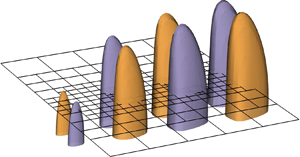
Figure 6. Isosurfaces of the negative and positive streamwise velocity (40 % of the magnitude, normalised by its maximum) of various unstable eigenmodes resembling the wake cells. For (a)  $r=1.1$, the fourth least-stable eigenmode of the direct operator resembles a modulation region, but in the wake of the small cylinder (purple/green isosurfaces). In (b–d) the second least-stable eigenmode (purple/orange isosurfaces) of the direct operator for $r=1.2$, $r=2$ and $r=4$, respectively. In addition, in (b) the green/blue isosurfaces indicate the negative and positive streamwise velocity of the third least-stable eigenmode for $r=1.2$. The black arrows indicate the flow direction.
4. Concluding remarks
This work investigates the global stability of the three-dimensional flow around a stepped cylinder for four different diameter ratios  $r=1.1$, $r=1.2$, $r=2$ and $r=4$, where $r$ is the ratio between the diameters of large and small cylinders. For each $r$, several Reynolds numbers are considered: $Re_D=40$, $Re_D=50$ and $Re_D=80$, where $D$ is the diameter of the large cylinder. First, the base flow is extracted from nonlinear DNS via SFD. Then, the eigenvalues, and corresponding eigenvectors, of the linearised NS operators are calculated. The AMR technique is used to design independent meshes for each nonlinear, linear direct and dual solution of the total 36 flow cases. The least-stable direct eigenmode is for all $r$ a three-dimensional eigenvector that is mainly localised in the wake of the large cylinder, resembling the L cell. It corresponds to the globally unstable mode of the flow past a circular cylinder with a $Re_{D,cr} \approx 47$. The structural sensitivity analysis confirms that the wavemaker region corresponds to the two lobes symmetrically placed across the separation bubble. The angular frequencies of the eigenvalues are in excellent agreement with oscillating states observed in the nonlinear DNS ( $St \approx 0.11$). The global instability is predominantly a two-dimensional mechanism, not affected by the presence of the junction, despite its extension.
However, the second least-stable eigenmode is interesting and relevant to consider for the various cases. The second supercritical Hopf bifurcation, expected at  $\widehat {Re}_{d,cr2} = Re_{D,cr} \cdot r$, occurs at a much lower Reynolds number due to three-dimensional effects and the N cell formation, especially at $r=2$ and $4$ (see figure 5). In addition, for all the ratios, as $Re_D$ increases, we observed an unstable eigenmode localised within the N cell, similar to the second unstable eigenmode for $r=2$ and $r=4$ shown in figure 6(c,d). This finding differs from the classification proposed by Lewis & Gharib (Reference Lewis and Gharib1992), who identified only two dominating modes when $r<1.25$. Our results indicate the onset of N cell shedding even for $r=1.1$ and $1.2$. This is a crucial observation, suggesting that the N cell tends to form for all $r>1$, with the S and L cells becoming dominant as the stepped cylinder approaches uniformity. Each cell undergoes a supercritical Hopf bifurcation, and the sequence of their transitions depends on the parameter $r$. It is worth noting that these findings arise from a modal linear global stability analysis and the emergence of nonlinearities as $Re_D$ increases may impact the N cell. Further validation is required at higher Reynolds numbers as $r$ approaches 1.
Interestingly, for  $r=1.1$ and $1.2$, the spanwise variation of the base flow vertical velocity exhibits a behaviour symmetric to the $z=0$ plane. This symmetry leads to the formation of an unstable eigenmode resembling an N cell but mirrored with respect to the $z=0$ plane, specifically within the wake of the small cylinder. It is worth noting that such a transitional cell, named N2, is reported here for the first time, as the geometries $r=1.1$ a $1.2$ have been barely studied in the past. The nonlinear results support the stability analysis in agreement with the formation mechanism of the N cell described by Massaro et al. (Reference Massaro, Peplinski and Schlatter2023d) in the turbulent regime for $r=2$. Further studies at a higher Reynolds number (for various diameter ratios) could clarify the interaction of the cells, with a particular focus on the persistence of the N2 cell for $r=1.1$ and $1.2$.
Funding
Financial support provided by the Knut and Alice Wallenberg Foundation is gratefully acknowledged. The simulations were performed on resources provided by the Swedish National Infrastructure for Computing (SNIC) at the PDC (KTH Stockholm) and NSC (Linköping University).
Declaration of interest
The authors report no conflict of interest.
Appendix
The DNS are conducted with a numerical framework that has been validated extensively in prior studies. The novel application of the AMR technique in the global stability analysis was introduced by Massaro et al. (Reference Massaro, Lupi, Peplinski and Schlatter2023a) and subsequently utilised by Massaro et al. (Reference Massaro, Lupi, Peplinski and Schlatter2023b). In addition, the design of the computational box was carefully assessed in earlier studies focused on the turbulent regime by Massaro et al. (Reference Massaro, Peplinski and Schlatter2023c,Reference Massaro, Peplinski and Schlatterd). Here, a similar assessment is presented for the low Reynolds number configuration.
Figure 1 shows the base flow extracted at a Reynolds number of  $Re_D=50>Re_{cr}$. In the numerical integration of the nonlinear NS equations, the SFD technique introduces a damping force $\boldsymbol {f}$ that damps the oscillations of the solution using a temporal low-pass filter (Åkervik et al. Reference Åkervik, Brandt, Henningson, Hæpffner, Marxen and Schlatter2006). The base flow is considered stabilised when the tolerance $\varepsilon = | \boldsymbol {u}-\boldsymbol {\omega } |_{L^2(\varOmega )}$ reaches a value $\varepsilon < 10^{-7}$. Achieving this level of convergence might require thousands of convective time units (based on the inflow velocity $U$ and the large cylinder diameter $D$), as discussed by Massaro et al. (Reference Massaro, Lupi, Peplinski and Schlatter2023a). Therefore, despite the low Reynolds number, reproducing figure 1 is computationally demanding. Nevertheless, the data for all geometries in figure 1 are compared with a case with the same setup but an extended spanwise dimension. Specifically, the small and large cylinders extend for $24D$ and $20D$, respectively (instead of $12D$ and $10D$). The two cases are referred to as G1 and G2. The results are compared in figure 7, where solid and dashed lines represent G1 ( $z/D \in [-20,24]$) and G2 ( $z/D \in [-10,12]$), respectively. The agreement between the results is excellent. In the front region of the cylinder (figure 7a), the solid and dashed lines closely match. Only for $r=2$ and $r=4$ do slight deviations appear in the peaks. Figure 7(b) displays the downward flow motion in the cylinder wake, a critical aspect given the conclusions drawn in the main text. Again, the solid and dashed lines exhibit excellent agreement. A slight deviation is noticeable for the red and green lines for $z/D<-5$. However, for G1, the negative peak of vertical velocity aligns well with the G2 case, with minor deviations within 2 % or less. Eventually, for a specific geometry ( $r=1.1$), the global stability analysis is also evaluated. The shape of the eigenmode remains substantially unaltered. The angular frequency and growth rate agree with the calculations in the smaller domain: $\sigma _{G1}=0.0152$ ( $\sigma _{G2}=0.0147$) and $\omega _{G1}=0.746$ ( $\omega _{G2}=0.749$). Hence, all global stability analyses presented in the paper are conducted using the mesh G2.

Figure 7. Effect of the spanwise extension of the computational domain on the base flow calculation. Spanwise variation of the vertical velocity component of the base flow at  $Re_D=50$ for the ratios $r=1.1$, $1.2$, $2$ and $4$. Two different locations are considered: $(x/D=-0.6,y=0)$ and $(x/D=3,y=0)$ in (a) and (b), respectively. The solid and dashed lines represent the G1 ( $z/D \in [-20,24]$) and G2 ( $z/D \in [-10,12]$) domains, respectively.


 Open access