


1. Introduction
Human physiology includes a wide number of examples of fluid flow through flexible-walled conduits including blood flow through the circulation (from rapid flow in the heart and large arteries to slow viscous flows through the capillaries), air flow through the lungs and upper airways, urine flows in the excretory system and peristaltic flows through the colon. In some circumstances these flows can exhibit instability, where the flow can interact with the flexible wall in a non-trivial way. Of particular interest in this study is the onset of self-excited oscillations, where the flow and the wall can spontaneously transition to an oscillatory limit cycle; in some cases this oscillation can even become chaotic. These oscillations manifest in physiological problems such as blood pressure measurement in the form of audible Korotkoff noises (Bertram, Raymond & Butcher Reference Bertram, Raymond and Butcher1989), and wheezing in the lung airways (Gavriely et al. Reference Gavriely, Shee, Cugell and Grotberg1989).
Self-excited oscillations in flexible-walled vessels can be studied experimentally using a Starling resistor, a deceptively simple device featuring liquid flow driven through a section of externally pressurised flexible tubing mounted between two rigid pipes. Originally used as a flow resistor in cardiac experiments (Knowlton & Starling Reference Knowlton and Starling1912), it has since become a canonical experiment for investigating fluid–structure interaction in its own right. In these experiments flow is driven using either a prescribed pressure or a prescribed flow rate, and the choice of set-up heavily influences the structure of the resulting oscillations. Results from the experiments are well summarised elsewhere (e.g. Bertram Reference Bertram2003; Grotberg & Jensen Reference Grotberg and Jensen2004; Heil & Hazel Reference Heil and Hazel2011), but we note that these self-excited oscillations occur in distinct frequency bands (Bertram, Raymond & Pedley Reference Bertram, Raymond and Pedley1990), and exhibit complicated nonlinear limit cycles which can be characterised using the methods of dynamical systems (Bertram, Raymond & Pedley Reference Bertram, Raymond and Pedley1991). Note that these experiments are typically conducted with relatively thick-walled tubes. For example, Bertram et al. (Reference Bertram, Raymond and Pedley1990, Reference Bertram, Raymond and Pedley1991) used tubes of wall thickness to baseline radius ratio of 0.3, while Bertram & Castles (Reference Bertram and Castles1999) used tubes with a thickness to radius ratio of 0.37.
There have been a number of theoretical studies of the Starling resistor set-up in an attempt to explain the underlying mechanisms leading to these different families of oscillation. Formulation of the full three-dimensional fluid structure interaction problem in a collapsible tube involves coupling unsteady Newtonian flow to a fully deformable elastic tube. While most theoretical models treat the tube wall as a thin shell, slightly reducing the complexity of the system, these models still require vast computational resources to resolve the unsteady oscillatory flow (Heil & Boyle Reference Heil and Boyle2010). Some analytical progress can be made in the limit of large membrane tension (where oscillations are high frequency, Whittaker et al. Reference Whittaker, Heil, Jensen and Waters2010), but this formulation is restricted to a state where the tube wall is almost uniform that has not yet been realised experimentally.
The flexible tubing used in Starling resistor experiments is typically much thicker than is appropriate to model using thin shell theory. To date, the only theoretical studies which incorporate a thick-walled tube have been restricted to steady flow configurations (Marzo, Luo & Bertram Reference Marzo, Luo and Bertram2005; Zhang, Luo & Cai Reference Zhang, Luo and Cai2018). In this paper we seek to address the stability of flow in a Starling resistor analogue with a thick hyperelastic wall, and investigate the role of wall thickness in promoting or inhibiting instability.
Given the computational difficulty and expense of full three-dimensional unsteady models, theoretical study has often focused on empirical lumped parameter or cross-sectionally averaged models for flow in collapsible tubes (e.g. Shapiro Reference Shapiro1977; Bertram & Pedley Reference Bertram and Pedley1982; Jensen Reference Jensen1990; Armitstead, Bertram & Jensen Reference Armitstead, Bertram and Jensen1996), which have replicated many of the features noted in Starling resistor experiments, such as non-uniform steady profiles and spontaneous transition to self-excited oscillations in distinct oscillation frequencies. However, the flow field in these models is still approximate and misses many of the subtleties of flow separation and energy dissipation.
To make progress in understanding the mechanisms of instability driving self-excited oscillations, a compromise system is needed which is less complicated than fully three-dimensional flow, but reduces the number of empirical assumptions needed for the lumped models. Pedley (Reference Pedley1992) proposed a two-dimensional analogue of the Starling resistor, consisting of a planar rigid channel where a section of one wall has been replaced by a flexible sheet. This set-up has since become the subject of a wide variety of computational (e.g. Luo & Pedley Reference Luo and Pedley1995, Reference Luo and Pedley1996, Reference Luo and Pedley1998, Reference Luo and Pedley2000; Heil Reference Heil2004) and theoretical studies (e.g. Jensen & Heil Reference Jensen and Heil2003; Guneratne & Pedley Reference Guneratne and Pedley2006; Stewart et al. Reference Stewart, Heil, Waters and Jensen2010; Pihler-Puzović & Pedley Reference Pihler-Puzović and Pedley2013). Despite reduced computational cost compared with the three-dimensional tube system, a full exploration of the parameter space for this collapsible channel analogue has not yet been attempted, although progress toward quantifying the mechanisms of instability has been made in various regions of the parameter space. For example, in the case of prescribed upstream flux (the subject of this study), Xu, Billingham & Jensen (Reference Xu, Billingham and Jensen2014) quantified the mechanism driving ‘sawtooth’ oscillations in the asymptotic limit of a long downstream rigid section, where the nonlinear oscillation is driven by the resonance of two distinct modes of perturbation (mode-1 and mode-2) of similar frequency and the same wavelength, coupled by sloshing flow in the downstream rigid section. Furthermore, Huang (Reference Huang2001) simplified the flux-driven collapsible channel system by imposing an external pressure gradient on the flexible wall, which facilitated decomposition of the oscillatory flow into a sum of sinusoidal modes. This analysis reveals an alternative mechanism of oscillatory instability, driven by an imbalance between (unstable) downstream propagating waves (which transfer energy from the flow to the wall) and (stable) upstream propagating waves (which transfer energy back from the wall to the fluid).
Further insights into the mechanisms of instability in these collapsible channel flows have been obtained using approximate one-dimensional models of the asymmetric channel system (derived using a flow-profile assumption, Stewart, Waters & Jensen Reference Stewart, Waters and Jensen2009; Stewart et al. Reference Stewart, Heil, Waters and Jensen2010; Xu, Billingham & Jensen Reference Xu, Billingham and Jensen2013; Xu et al. Reference Xu, Billingham and Jensen2014; Xu & Jensen Reference Xu and Jensen2015; Stewart Reference Stewart2017). In particular, a detailed exploration of the parameter space for flux-driven oscillations with constant external pressure was presented by Stewart (Reference Stewart2017), where he found that when the fluid is inviscid, steady states only exist above a critical value of the membrane tension (for all other parameters held fixed), with a stable branch and an unstable branch (where the unstable branch is more collapsed than the stable branch). This critical point appears to be an organising centre of the dynamical system, in that many of the unsteady features of the system originate close to this point (such as the neutral curves for the two different families of self-excited oscillations). The importance of the critical point for inviscid steady states has previously been elucidated by Xu et al. (Reference Xu, Billingham and Jensen2013), who used an external pressure gradient. Stewart (Reference Stewart2017) also described another branch of steady solutions maintained by viscous effects, which becomes increasingly collapsed as the wall tension is reduced. As the Reynolds number increases this viscous branch of steady solutions merges with one of the (essentially) inviscid branches. When the viscous branch merges smoothly with the stable inviscid branch then the stable steady state is unique. However, the other possibility is that the viscous branch merges with the unstable inviscid branch in a limit point bifurcation, where the system then exhibits three co-existing steady states across a narrow region of the parameter space: the stable inviscid solutions become the upper branch, the unstable inviscid solutions become the intermediate branch and the stable viscous solutions become the lower branch. Stewart (Reference Stewart2017) also showed that the lower branch of steady solutions can become unstable to two distinct families of self-excited oscillation, with high and low frequency, respectively. However, in addition to the flow-profile assumption, this study considered the flexible wall to be a thin (massless) pre-stressed membrane with no bending rigidity. To overcome these simplifications, this study revisits the predictions of Stewart (Reference Stewart2017) by modelling the flexible wall as a pre-tensioned hyperelastic solid, using the finite element method to compute the fully two-dimensional steady wall and flow profiles, and test their stability to time-dependent perturbations using a fully two-dimensional eigensolver. Our new model includes the wall thickness and wall mass as explicit parameters, and we investigate their influence on the predictions below.
Another approach for theoretical modelling of this collapsible channel system has very recently been presented by Wang, Luo & Stewart (Reference Wang, Luo and Stewart2021a,Reference Wang, Luo and Stewartb), who treat the flexible wall as an asymptotically thin beam with resistance to both bending and stretching but with no pre-tension (based on an earlier model by Cai & Luo Reference Cai and Luo2003; Luo et al. Reference Luo, Cai, Li and Pedley2008). Using fully nonlinear simulations of this model, they identified a similar three-branch steady system for some parameters, showing that both the upper and lower branches of oscillation could (independently) become unstable to self-excited oscillations (Wang et al. Reference Wang, Luo and Stewart2021a) and these families of oscillations could merge together for low external pressures (Wang et al. Reference Wang, Luo and Stewart2021b). In this case the upper branch instability is restricted to a region in the near neighbourhood of that which exhibits multiple steady states (Wang et al. Reference Wang, Luo and Stewart2021b). In this study we also isolate a family of upper branch instabilities, but show that these are not limited to the region with multiple steady states but are instead unstable well away from the region of parameter space which exhibits instabilities of the lower steady branch (see § 3.4 below).
The role of wall mass in the onset of self-excited oscillations in flexible-walled vessels has already been considered for the flexible wall modelled as a thin membrane. For example, in the asymmetric channel system, Luo & Pedley (Reference Luo and Pedley1998) coupled the heavy membrane to fully two-dimensional (unsteady) flow, showing that increasing the wall mass expands the region of parameter space where the system exhibits the primary global instability, and also results in an additional high-frequency oscillatory mode (superimposed on the fundamental mode) which eventually grows to dominate the lower-frequency mode. Also, Pihler-Puzović & Pedley (Reference Pihler-Puzović and Pedley2014) investigated this channel system using interactive boundary layer theory, showing that wall mass drives an oscillatory instability which is always unstable in the presence of a cross-stream pressure gradient across the core flow (the system is always neutrally stable with no cross-stream gradient). Finally, Walters, Heil & Whittaker (Reference Walters, Heil and Whittaker2018) considered the role of wall mass in a thin shell model of flow in a collapsible tube in the limit of large pre-stress (where the tube is almost uniform), finding that wall inertia destabilises the primary mode of instability of the system while also lowering the corresponding oscillation frequency.
In this paper we consider the planar channel analogue of the Starling resistor introduced by Pedley (Reference Pedley1992), and propose a new numerical method to solve the combined fluid and solid problem based on that developed by Snoeijer et al. (Reference Snoeijer, Pandey, Herrada and Eggers2020) (which already has application to viscoelastic fluids, Eggers, Herrada & Snoeijer Reference Eggers, Herrada and Snoeijer2020). The model formulation is described in § 2, highlighting the novel features of the numerical method. In particular, we treat the elastic solid as a pre-tensioned hyperelastic material of uniform initial thickness with non-negligible density and subject to a uniform external pressure. We validate this numerical method against the steady predictions of Heil (Reference Heil2004), who considered an identical set-up with a thin shell model for the wall (§ 3.1), use unsteady simulations to examine the transition between the upper and lower branches of steady solutions (§ 3.2), examine the onset of self-excited oscillations from these steady solutions (§ 3.3), before using our new model to examine the role of membrane pre-tension (§ 3.4), the dynamics of oscillations growing from the upper branch of steady solutions (§ 3.5) as well as the role of wall thickness (§ 3.6) and wall inertia (§ 3.7) on the nonlinear steady solutions and the accompanying onset of oscillation.
2. Model formulation
We consider the configuration sketched in figure 1, where an incompressible Newtonian fluid is flowing through a planar rigid (two-dimensional) channel of uniform internal width  $h$. An interior section of length $L$ is removed from the upper wall of the channel and replaced by a pre-tensioned elastic solid of (initially) uniform thickness $e$, subject to a passive external gas at uniform pressure, $P_{ext}$. This elastic wall can be deformed by the load of the external gas and by the fluid traction. The rigid sections upstream and downstream of the compliant segment are of length $L_1$ and $L_2$, respectively. In this case the flow is driven by a prescribed upstream flux $q$, while the fluid pressure at the downstream end of the channel can be set to zero without loss of generality. The stability of this fluid–structure interaction problem has already been studied extensively using reduced models for the elastic wall (e.g. Luo & Pedley Reference Luo and Pedley1996; Jensen & Heil Reference Jensen and Heil2003; Luo et al. Reference Luo, Cai, Li and Pedley2008; Stewart Reference Stewart2017). In this work, we model the wall as a continuum hyperelastic solid of finite thickness, with no simplifications or reductions. Our formulation is based on first-order elasticity (elastic strain energy function dependent on the strain tensor), which places some restrictions on the boundary conditions that can be imposed.

Figure 1. Sketch of the flow geometry considered in this study.
2.1. Equations of motion
The fluid domain  $\varOmega _1$ is described by the planar coordinates $\boldsymbol {x}=x\boldsymbol {e}_x + y\boldsymbol {e}_y$, where $x$ parametrises the lower wall of the channel, with $x=0$ at the intersection between the upstream rigid segment and the compliant segment, while $y$ parametrises the direction normal to the entirely rigid wall pointing into the fluid (in the plane of the channel). The solid domain $\varOmega _2$ is measured relative to a reference configuration parametrised by the coordinates $\boldsymbol {X}=X\boldsymbol {e}_x + Y\boldsymbol {e}_y$, where $X$ parametrises the lower surface of the flat wall and $Y$ parametrises the direction pointing into the wall (in the plane of the channel).
The conservation of mass and momentum equations in the fluid ( $i=1$) and solid ( $i=2$) subdomains are given by
 \begin{gather} {\boldsymbol{\nabla}}\boldsymbol{\cdot}\boldsymbol{v}_i = 0, \quad (i=1,2), \end{gather}
 \begin{gather}\rho_i\left(\frac{\partial \boldsymbol{v}_i}{\partial t} + \left(\boldsymbol{v}_i\boldsymbol{\cdot} {\boldsymbol{\nabla}}\right)\boldsymbol{v}_i \right) = {\boldsymbol{\nabla}}\boldsymbol{\cdot}\boldsymbol{\sigma}_{i}, \quad (i=1,2), \end{gather}
where  $\rho _i$ is the density, $\boldsymbol{\mathsf{I}}$ is the identity tensor, $\boldsymbol {v}_i$ the velocity field and $\boldsymbol {\sigma }_i$ is the stress tensor of material $i$ (
$i$ ( $i=1,2$). Each stress tensor depends on the characteristics of the material through a constitutive model. In region 1 we consider an incompressible Newtonian fluid, where this stress tensor takes the form
 \begin{equation} \boldsymbol{\sigma}_{1}={-}p_1 \boldsymbol{\mathsf{I}}+ \eta_1\left({\boldsymbol{\nabla}}\boldsymbol{v}_1+{\boldsymbol{\nabla}}\boldsymbol{v}_1^{\rm T}\right), \end{equation}
where  $p_1$ is the fluid pressure and $\eta _1$ is the fluid viscosity. In region 2 we consider a neo-Hookean (hyperelastic) solid which has a pre-stress, $\boldsymbol {\sigma }_{2p}^{(0)}$, in the initial undeformed state, where the stress tensor is given by (Snoeijer et al. Reference Snoeijer, Pandey, Herrada and Eggers2020)
 \begin{equation} \boldsymbol{\sigma}_{2}={-}p_2 \boldsymbol{I}+ \mu_2 \left(\boldsymbol{F}\boldsymbol{\cdot}\boldsymbol{F}^{T}-\boldsymbol{\mathsf{I}}\right)+\boldsymbol{F} \boldsymbol{\cdot} \boldsymbol{\sigma}_{2p}^{(0)} \boldsymbol{\cdot} \boldsymbol{F}^{\rm T}, \end{equation}
where  $p_2$ is the solid pressure, $\mu _2$ is the elastic shear modulus, ${\boldsymbol {x}}({\boldsymbol {X}},t)$ is the position of a material point after deformation of the solid and $\boldsymbol {F}=\partial \boldsymbol {x}/\partial \boldsymbol {X}$ is the deformation gradient tensor. In the initial state, $\boldsymbol {x}=\boldsymbol {X}$ and $\boldsymbol {F}\boldsymbol {\cdot }\boldsymbol {F}^{\rm T}=\boldsymbol{\mathsf{I}}$. To make a connection between the Eulerian formulation for the conservation of mass and momentum equations for the solid ((2.1) with $i=2$) and the Lagrangian formulation for the elastic stress, we need to determine the deformation generated by transport by the solid velocity $\boldsymbol {v}_2$. This is achieved using the inverse Lagrangian map $\boldsymbol {X}({\boldsymbol {x}},t)$ (Kamrin, Rycroft & Nave Reference Kamrin, Rycroft and Nave2012), which satisfies
 \begin{equation} \frac{\partial \boldsymbol{X}}{\partial t} + \boldsymbol{v}_2\boldsymbol{\cdot}{\boldsymbol{\nabla}}\boldsymbol{X} = 0, \end{equation}
because the reference coordinates are invariant under the flow.
Given the bi-dimensionality of the problem, the material points can be expressed in Cartesian coordinates and so the velocity vectors can be written as
 \begin{equation} \boldsymbol{v}_i = v_{yi}\boldsymbol{e}_y + v_{xi}\boldsymbol{e}_x, \quad (i=1,2), \end{equation}
while the stress tensors can be written as
 \begin{equation} \boldsymbol{\sigma} = \sigma_{yy}\boldsymbol{e}_y\otimes\boldsymbol{e}_y + \sigma_{yx}\boldsymbol{e}_y\otimes\boldsymbol{e}_x + {\sigma_{xy}\boldsymbol{e}_x\otimes\boldsymbol{e}_y} + \sigma_{xx}\boldsymbol{e}_x\otimes\boldsymbol{e}_x, \end{equation}
and finally the deformation tensor in the solid can be written as
 \begin{equation} \boldsymbol{F} = \frac{\partial y}{\partial Y}\boldsymbol{e}_y\otimes\boldsymbol{e}_y + \frac{\partial y}{\partial X}\boldsymbol{e}_y\otimes\boldsymbol{e}_x + \frac{\partial x}{\partial Y}\boldsymbol{e}_x\otimes\boldsymbol{e}_y +\frac{\partial x}{\partial X}\boldsymbol{e}_x\otimes\boldsymbol{e}_x. \end{equation}
In the undeformed position the elastic solid is subject to an initial longitudinal tension,  $T_o$, and therefore the initial stress is $\boldsymbol {\sigma }_{2p}^{(0)}=(T_0/e)\boldsymbol {e}_x\otimes \boldsymbol {e}_x$.
For the elastic domain, it is convenient to replace the incompressibility equation based on the velocity field ((2.1a) with  $i=2$) by a constraint involving the deformation tensor $\boldsymbol {F}$ (Snoeijer et al. Reference Snoeijer, Pandey, Herrada and Eggers2020) in the form
 \begin{equation} \det(\boldsymbol{F}) = \left(\frac{\partial y}{\partial Y} \frac{\partial x}{\partial X}-\frac{\partial y}{\partial X} \frac{\partial x}{\partial Y}\right)= 1. \end{equation}
To impose the upstream flux boundary condition for the liquid, we impose a Poiseuille profile at the channel entrance,  $x=-L_1$, in the form
 \begin{equation} v_{1x}=\frac{6q}{h^3} \, y(h-y),\quad v_{1y}=0, \quad (x={-}L_1, 0\leqslant y \leqslant h).\end{equation}
At the channel exit,  $x=L+L_2$, we impose zero fluid pressure, $p_1=0$. Along the entirely rigid wall we apply no-slip conditions in the form
 \begin{equation} v_{x1}=v_{y1}=0, \quad (y=0, -L_1 \leqslant x \leqslant L+L_2). \end{equation}
Similarly, along the rigid parts of the upper wall we apply no-slip boundary conditions in the form
 \begin{equation} v_{x1}=v_{y1}=0, \quad (y=h, -L_1 \leqslant x \leqslant 0, x\geqslant L). \end{equation}
We assume that the flexible surface (where the elastic solid and the fluid interact) can be written as a function of  $x$ (i.e. the surface does not overturn or expand beyond the range $0\leqslant x\leqslant L$), so that $y=h_1(x,t)$. Across this interface we impose that the velocity field must be continuous, in the form
 \begin{equation} v_{x1}=v_{x2},\quad v_{y1}=v_{y2}, \quad (y=h_1, 0\leqslant x\leqslant L), \end{equation}
and impose a balance of normal and tangential stresses between the solid and the fluid, in the form
 \begin{equation} \boldsymbol{n}_1\boldsymbol{\cdot}({\boldsymbol{\sigma}}_{1}-\boldsymbol{\sigma}_{2})\boldsymbol{\cdot} \boldsymbol{n}_1=0,\quad \boldsymbol{t}_1\boldsymbol{\cdot}({\boldsymbol{\sigma}}_{1}-\boldsymbol{\sigma}_{2}) \boldsymbol{\cdot} \boldsymbol{n}_1=0, \end{equation}
where
 \begin{equation} \boldsymbol{n}_1 = \frac{\boldsymbol{e}_y-\boldsymbol{e}_x h_{1,x}}{(1+h_{1,x}^2)^{1/2}},\quad \boldsymbol{t}_1 = \frac{\boldsymbol{e}_x+\boldsymbol{e}_y h_{1,x}}{(1+h_{1,x}^2)^{1/2}}, \end{equation}
are normal and tangential vectors to the surface  $y=h_1(x,t)$, respectively, and the subscript $x$ represents a derivative with respect to $x$. In this first-order elasticity approach we enforce no deformation along the surfaces where the elastic material is adhered to the rigid walls (i.e. the displacement of the solid is clamped along two edges of the rectangle in contact with the rigid walls), in the form
 \begin{equation} v_{2x}=v_{2y}=0,\quad Y=y,\quad X=x, \quad (x=0, x=L \ \text{with} \ h \leqslant y\leqslant h+e). \end{equation}
However, our approach does not replicate the resistance to bending of a classical Euler–Bernoulli beam. This would require second-order (or strain gradient) elasticity, where the elastic strain energy function is assumed to depend on both the strain tensor and the strain gradient tensor (Bertram & Forest Reference Bertram and Forest2020). In that case one must impose additional constraints on the contact between the beam and the rigid wall e.g. conditions on the derivatives of displacement, such as prescribed slope or torque. Finally, we denote the external surface of the flexible wall as  $y=h_2(x,t)$, $(0\leqslant x\leqslant L$) and impose that the normal and tangential elastic stresses are balanced with the external pressure, in the form
 \begin{equation} \boldsymbol{n}_2\boldsymbol{\cdot}({\boldsymbol{\sigma}}_{2}-P_{ext}\boldsymbol{\mathsf{I}})\boldsymbol{\cdot} \boldsymbol{n}_2=0,\quad \boldsymbol{t}_2\boldsymbol{\cdot}({\boldsymbol{\sigma}}_{2}) \boldsymbol{\cdot} \boldsymbol{n}_2=0, \end{equation}
where
 \begin{equation} \boldsymbol{n}_2 = \frac{\boldsymbol{e}_y-\boldsymbol{e}_x h_{2,x}}{(1+h_{2,x}^2)^{1/2}},\quad \boldsymbol{t}_2 = \frac{\boldsymbol{e}_x+\boldsymbol{e}_y h_{2,x}}{(1+h_{2,x}^2)^{1/2}}, \end{equation}
are normal and tangential vectors to the surface  $y=h_2(x,t)$.
2.2. Mapping technique
The numerical technique used in this study is a variation of that developed by Herrada & Montanero (Reference Herrada and Montanero2016) for interfacial flows and extended by Snoeijer et al. (Reference Snoeijer, Pandey, Herrada and Eggers2020) to apply to hyperelastic solids. The spatial domain occupied by the fluid,  $\varOmega _1(t)$, is mapped onto a rectangular domain (parametrised by Cartesian coordinates $\xi _1$ and $\chi _1$, where $\xi _1$ parametrises the lower rigid wall and $\chi _1$ parametrises the channel inlet) by means of a non-singular mapping
 \begin{equation} y=f_1(\xi_1,\chi_1,t),\quad x=g_1(\xi_1,\chi_1,t),\quad [{-}L_1\leqslant \xi_1\leqslant L+L_2]\times[0\leqslant \chi_1\leqslant 1], \end{equation}
where the shape functions  $f_1$ and $g_1$ are obtained as part of the solution. In order to capture large anisotropic deformations, the following quasi-elliptic transformation (Dimakopoulos & Tsamopoulos Reference Dimakopoulos and Tsamopoulos2003) was applied:
 \begin{gather} g_{22}\frac{\partial^2 f_{1}}{\partial \xi_1^2}+g_{11}\frac{\partial^2 f_{1}}{\partial \chi_1^2}-2g_{12}\frac{\partial^2 f_{1}}{\partial \xi_1\partial \chi_1} = Q, \end{gather}
 \begin{gather}g_{22}\frac{\partial^2 g_{1}}{\partial \xi_1^2}+g_{11}\frac{\partial^2 g_{1}}{\partial \chi_1^2}-2g_{12}\frac{\partial^2 g_{1}}{\partial \xi_1\partial \chi_1}= 0, \end{gather}
where the coefficients take the form
 \begin{equation} g_{11}=\left(\frac{\partial g_{1}}{\partial \xi_1}\right)^2\!+\!\left(\frac{\partial f_{1}}{\partial \xi_1}\right)^2, \quad g_{22}=\left(\frac{\partial g_{1}}{\partial \chi_1}\right)^2\!+\!\left(\frac{\partial f_{1}}{\partial \chi_1}\right)^2,\quad g_{12}=\frac{\partial g_{1}}{\partial \chi_1}\frac{\partial g_{1}}{\partial \xi_1}+\frac{\partial f_{1}}{\partial \chi_1}\frac{\partial f_{1}}{\partial \xi_1}, \end{equation}
with
 \begin{equation} Q={-}\left(\frac{\partial D_{1}}{\partial \chi_1}\frac{\partial f_{1}}{\partial \xi_1}-\frac{\partial D_{1}}{\partial \xi_1}\frac{\partial f_{1}}{\partial \chi_1}\right )\frac{J}{D_1}, \quad J= \frac{\partial g_{1}}{\partial \chi_1}\frac{\partial f_{1}}{\partial \xi_1}-\frac{\partial g_{1}}{\partial \xi_1}\frac{\partial f_{1}}{\partial \chi_1}, \end{equation}
and
 \begin{equation} D_1=\epsilon_p\sqrt{\left.\left[\left(\frac{\partial f_{1}}{\partial \xi_1}\right)^2+\left(\frac{\partial g_{1}}{\partial \xi_1}\right)^2\right]\right/\left[\left(\frac{\partial f_{1}}{\partial \chi_1}\right)^2+\left(\frac{\partial g_{1}}{\partial \chi_1}\right)^2\right]}+(1-\epsilon_p). \end{equation}
In the above expressions,  $\epsilon _p$ is a free parameter between 0 and 1 where the case $\epsilon _p=0$ corresponds to the classical elliptical transformation. All the simulations in this work were conducted using $\epsilon _p=0.2$. Although there is no overturning in the wall profiles for the cases analysed in this work, this transformation of the liquid domain facilitates the analysis of more complicated geometries. For example, it has been successfully used to describe pinch-off in pendant drops (Ponce-Torres et al. Reference Ponce-Torres, Rubio, Herrada, Eggers and Montanero2020).
The spatial domain occupied by the elastic solid in the current stage,  $\varOmega _2(t)$, and in the initial stage, $\varOmega _{2o}$, are also mapped onto rectangular domains (parametrised by Cartesian coordinates $\xi _2$ and $\chi _2$, where $\xi _2$ parametrises the lower surface of the flexible wall and $\chi _2$ parametrises the edges in contact with the rigid segments of the channel) by means of non-singular mappings in the form
 \begin{equation} \left.\begin{gathered} y=f_2(\xi_2,\chi_2,t),\quad x=g_2(\xi_2,\chi_2,t),\\ Y=F_2(\xi_2,\chi_2,t),\quad X=G_2(\xi_2,\chi_2,t),\quad [0\leqslant \xi_2\leqslant L]\times [0\leqslant \chi_2\leqslant 1], \end{gathered}\right\} \end{equation}
where again the functions  $f_2$, $g_2$, $F_2$ and $G_2$ should be obtained as a part of the solution. To determine these functions, the following equations have been used:
 \begin{gather} g_2 =\xi_2, \end{gather}
 \begin{gather}F_2 = h+ e\chi_2. \end{gather}
Note that (2.8a) guarantees that the discretisation used for the variable  $\xi _2$ is automatically applied to variable $x$. Finally, (2.8b) indicates that at the initial stage the elastic part of the upper channel wall is a perfect rectangle of uniform width $e$.
$e$.
Some additional boundary conditions for the shape functions are needed to close the problem. At the channel entrance, we impose
 \begin{equation} g_1={-}L_1,\quad f_1=h\chi_1, \quad (x =\xi_1={-}L_1), \end{equation}
while at the channel exit, we use
 \begin{equation} g_1=L+L_2,\quad f_1=h\chi_1, \quad (x =\xi_1= L + L_2). \end{equation}
On the lower wall, we impose
 \begin{equation} g_1=\xi_1,\quad f_1=0, \quad (y =\chi_1=0), \end{equation}
while on the rigid parts of the upper channel wall, we use
 \begin{equation} g_1=\xi_1,\quad f_1=h, \quad ({-}L_1\leqslant x=\xi_1\leqslant0,\ x=\xi_1\geqslant L,\ y=h). \end{equation}
At the flexible surface, we also impose
 \begin{equation} f_1=f_2,\quad g_1=g_2, \quad (0\leqslant x=\xi_1=\xi_2\leqslant L, y=h_{1}(x,t), \chi_1=1, \chi_2=0). \end{equation}
Finally, we enforce no displacement of the elastic solid along the two edges of the rectangle in contact with the rigid walls, in the form
 \begin{equation} \left.\begin{gathered} g_2=G_2=\xi_2,\quad f_2=F_2=h+e\chi_2, \\ (x=\xi_2=0, x=\xi_2=L, h \leqslant y\leqslant (h+e), 0 \leqslant \chi_2\leqslant~1). \end{gathered}\right\} \end{equation}
 Figure 2 shows an example of the mappings used in this work. The green (magenta) lines represent the liquid (solid) mesh in the real space (bottom panel) and in the computational domain (top panel). The unknown variables in the liquid domain are  $f_1$, $g_1$, $p_1$, $v_{1x}$ and $v_{1y}$ while the unknown variables in the solid domain are $f_2$, $g_2$, $p_2$, $v_{2x}$, $v_{2y}$, $F_2$ and $G_2$. All the derivatives appearing in the governing equations are expressed in terms of $\chi$, $\xi$ and $t$. These mappings are applied to the governing equations (2.1) and the resulting equations are discretised in the $\chi$-direction with $n_{\chi _1}$ and $n_{\chi _2}$ Chebyshev spectral collocation points in the liquid and solid domains, respectively. Conversely, in the $\xi$-direction we use fourth-order finite differences with $n_{\xi _1}$ and $n_{\xi _2}$ equally spaced points in the liquid and solid domains, respectively. The results presented in this work were carried out using $n_{\xi _1}=641$, $n_{\xi _2}=201$, $n_{\chi _1}=19$ and $n_{\chi _2}=14$. In the Appendix we demonstrate that the eigenvalues characterising the linear modes do not change significantly when the number of grid points is increased.

Figure 2. Computational subdomains and grids for the original and mapped variables.
2.3. Steady solutions
Steady solutions of the nonlinear equations (2.1) with all variables independent of time are obtained by solving all equations simultaneously (a so-called monolithic scheme) using a Newton–Raphson technique. One of the main characteristics of this procedure is that the elements of the Jacobian matrix  $\mathcal {J}^{(p,q)}$ of the discretised system of equations are obtained by combining analytical functions and collocation matrices. This allows us to take advantage of the sparsity of the resulting matrix to reduce the computation time on each Newton step.
We denote the steady solution of the system with the subscript  $b$. We trace the steady solutions as a function of the model parameters and quantify using the minimal and maximal positions of the lower surface of the flexible wall, denoted as
 \begin{equation} {\hat{h}}_{min}=\min\limits_{x}\left(\frac{h_{1b}}{h}\right) \quad \text{and} \quad {\hat{h}}_{max}=\max\limits_{x}\left(\frac{h_{1b}}{h}\right). \end{equation}
2.4. Small amplitude perturbations
To test the stability of a given steady state we calculate the linear two-dimensional global modes by assuming the temporal dependence
 \begin{equation} \varPsi(x,y;t)=\varPsi_b(x,y)+\epsilon \, \delta \varPsi(x,y){\rm e}^{-{\rm i}\omega t}, \quad (\epsilon\ll 1), \end{equation}
where  $\varPsi (x, y; t)$ represents any dependent variable while $\varPsi _b(x, y)$ and $\delta \varPsi (x, y)$ denote the base (steady) solution and the spatial dependence of the eigenmode for that variable, respectively, while $\omega =\omega _r+\textrm {i}\omega _i$ is the frequency (an eigenvalue). Both the eigenfrequencies and the corresponding eigenmodes are calculated as a function of the governing parameters. The dominant eigenmode is that with the largest growth factor $\omega _i$. If that growth factor is positive, the base flow is asymptotically unstable.
As explained by Herrada & Montanero (Reference Herrada and Montanero2016), the numerical procedure used to solve the steady problem can be easily adapted to solve the eigenvalue problem which determines the linear global modes of the system. In this case, the temporal derivatives are computed assuming the temporal dependence (2.11). The spatial dependence of the linear perturbation  $\delta \varPsi ^{(q)}$ is the solution to the generalised eigenvalue problem $\mathcal {J}^{(p,q)}_b\delta \varPsi ^{(q)}=i\omega \mathcal {Q}^{(p)}_b \delta \varPsi ^{(q)}$, where $\mathcal {J}^{(p,q)}_b$ is the Jacobian of the system evaluated with the basic solution $\varPsi _b^{(q)}$, and $\mathcal {Q}^{(p,q)}_b$ accounts for the temporal dependence of the problem. This generalised eigenvalue problem is solved using Matlab eigs function.
2.5. Fully nonlinear dynamical simulations
The numerical method can be extended to compute unsteady solutions of the full nonlinear equations (2.1). Temporal derivatives are discretised using second-order backwards differences and at each time step the resulting system of (nonlinear algebraic) equations is solved using the Newton–Raphson technique (as in § 2.3). Simulations employ the same mesh as the steady simulations with a fixed timestep of  $\Delta t = 0.0125$ required to capture the strong oscillations observed in the fully saturated nonlinear regime (this translates into approximately 640 timesteps per period for the oscillation shown in figure 12 below). We have verified that the nonlinear predictions are unchanged when the timestep is reduced to $\Delta t = 0.0075$. Given the large number of timesteps required, these simulations are much more computationally expensive than the global stability eigensolver and so only two relevant cases will be considered to support the global stability analysis (see figures 6 and 12 below). For example, the nonlinear simulation described in § 3.5 takes more than one week to reach the corresponding nonlinear limit cycle, while for the same machine the computation of the eigenvalues takes just a few minutes.
2.6. Control parameters
To non-dimensionalise the system we scale all lengths on the baseline channel width  $h$, velocities on the mean inlet speed $q/h$, time on $h^2/q$, the fluid stress on the viscous scale $\eta _1 q/h^2$ and the solid stress on the elastic shear modulus $\mu _2$. The solutions are characterised by the dimensionless profile of the interface between fluid and solid ${\hat {h}}_{b1} = h_{b1}/h$, the dimensionless frequency ${\hat \omega } = {\omega }q/h^2$ and the dimensionless eigenfunction profile of the surface between the fluid and the solid, denoted $\widehat {\delta h}_1 = (\delta h_1)/h$. As is conventional in this literature, a wall profile is termed as mode- $n$ if $\widehat {\delta h}_1$ has $n$ extrema across the compliant segment. The resulting problem is governed by six dimensionless parameters,
 \begin{align} Re=\frac{\rho_1 q}{\eta_1},\quad Q=\frac{\eta_1 q}{h^2\mu_2}, \quad \hat{p}_{ext}=\frac{{P}_{ext}}{\mu_2}, \quad \hat{T}_0=\frac{T_0}{h\mu_2}, \quad \hat{e}=\frac{e}{h}, \quad \hat{\rho}=\frac{\rho_2 q^2}{h^2\mu_2}, \end{align}
representing the Reynolds number, the ratio of the viscous stresses in the fluid to the elastic shear stresses in the wall, the dimensionless external pressure, the dimensionless longitudinal pre-tension, the dimensionless thickness of the flexible wall and the ratio between the inertial and the elastic forces in the solid. The dimensionless system also involves three geometrical factors,
 \begin{equation} \hat{L}_1=\frac{L_1}{h}, \quad \hat{L}=\frac{L}{h}, \quad \hat{L}_2=\frac{L_2}{h}, \end{equation}
which will be held constant throughout this study.
3. Results
In this section we predict the stability of flow through a flexible-walled channel with a hyperelastic wall. We first validate our model against published results for steady flow through channels with thin flexible walls presented by Heil (Reference Heil2004) (§ 3.1) and then examine the unsteady transition from beyond the upper branch limit point to the lower branch of steady solutions (§ 3.2). We then consider the onset of self-excited oscillations associated with these steady states across the parameter space spanned by Reynolds number and external pressure (§ 3.3), before examining the role of wall pre-tension (§ 3.4), the nonlinear limit cycles of oscillations which grow from the upper branch of steady solutions (§ 3.5), as well as the role of wall thickness (§ 3.6) and the role of wall inertia (§ 3.7) in the onset of these oscillations. Following Heil (Reference Heil2004), in all simulations we hold  ${\hat {L}}_{1}=1$, ${\hat {L}}=5$, ${\hat {L}}_2=10$ and fix the fluid–structure interaction parameter as $Q=0.01$, indicating that elastic stresses dominate viscous stresses. In the results below we vary the Reynolds number $Re$, external pressure ${\hat {p}}_{ext}$, the wall pre-tension ${\hat {T}}_0$ (§ 3.4), the wall thickness ${\hat {e}}$ (§ 3.6) and the wall inertia parameter ${\hat {\rho }}$ (§ 3.7).
3.1. Steady flow with thin flexible walls
We first compare the predictions from our numerical method against the predictions of Heil (Reference Heil2004), who studied the flow through the geometry shown in figure 1 but where his elastic wall was modelled using (geometrically nonlinear) shell theory, intended to capture large displacements in the elastic solid. Our choice of non-dimensionalisation is identical to Heil (Reference Heil2004), with the exception that he defines a membrane pre-stress  $\sigma _0$, which is related to our membrane pre-tension parameter through
 \begin{equation} \sigma_0 =\frac{\hat{T}_0}{\hat{e}}. \end{equation}
To compare with the predictions of Heil (Reference Heil2004), we consider a small wall thickness  ${\hat {e}}=0.01$. We then use pre-tension ${\hat {T}}_0=10$ to ensure that ${\sigma _0}=1000$, as used by Heil (Reference Heil2004). Since the inertia of the solid was neglected in that work we also set $\hat {\rho }=0$ in our simulations in this section (we consider non-zero wall inertia in § 3.7 below).
In order to compare the predictions of our model with those of Heil (Reference Heil2004), in figure 3 we illustrate the steady flow field computed using our method (figure 3a) and the steady flow field obtained using the model of Heil (Reference Heil2004) (figure 3b). We observe excellent quantitative agreement between the two approaches, not only in the pressure distribution but also in the streamlines, where both exhibit a recirculating flow separation region downstream of the point of strongest wall collapse. Quantitatively, we compute the relative error in the maximal (minimal) fluid pressure as  $0.2028\,\%$ ( $0.2089\,\%$) between our approach and the data from Heil (Reference Heil2004) for these parameter values.

Figure 3. Streamlines and pressure contours for the steady solution computed at fixed Reynolds number ( $Re=500$) and fixed external pressure ( $\hat {p}_{ext}=3.204$) obtained from: (a) the present model; (b) the model of Heil (Reference Heil2004). Here, ${\hat {T}}_0=10$, ${\hat {e}}=0.01$ and ${\hat {\rho }}=0$.
Following Heil (Reference Heil2004), in figure 4 we characterise the steady solutions of the system by the minimal ( ${\hat {h}}_{min}$) and maximal ( ${\hat {h}}_{max}$) channel width as a function of the model parameters. Similar to previous studies in collapsible channels (Luo & Pedley Reference Luo and Pedley2000; Heil Reference Heil2004; Stewart Reference Stewart2010, Reference Stewart2017) and collapsible tubes (Heil & Boyle Reference Heil and Boyle2010), we find that for sufficiently large Reynolds numbers the system can admit multiple steady solutions at the same point in parameter space. For example, figure 4(a) shows that the minimum dimensionless channel width ( ${\hat {h}}_{min}$), when plotted as a function of the external pressure, $\hat {p}_{ext}$, lies on a curve with three branches connected by two limit points (or fold bifurcations), where these three branches are labelled I, II and III. In order to quantify the difference between our results and those of Heil (Reference Heil2004), figure 4(b) compares our prediction of the intermediate and lower steady branches as a function of external pressure with those depicted in figure 4 of Heil (Reference Heil2004) (for the same parameter values). We observe excellent quantitative agreement, although the two approaches do diverge slightly for larger external pressures when the channels are significantly more collapsed, which we attribute to the increased prominence of the differences between the wall models. Furthermore, we also produce the same plot for a smaller Reynolds number ( $Re=250$) for which the wall profile is unique for all external pressures. Again we see excellent quantitative agreement between the models, with a slight divergence as the channel becomes increasingly collapsed.

Figure 4. Nonlinear steady solutions of the model for fixed Reynolds number ( $Re=500$) and pre-tension ( ${\hat {T}}_0=10$) showing: (a) the maximal and minimal channel widths as a function of the external pressure; (b) the channel width at $\hat {x}=3.5$ as a function of the external pressure (black line), compared with the prediction from figure 4 in Heil (Reference Heil2004) (green line). The dotted lines in (b) show the comparison the present model (black) with Heil (Reference Heil2004) (green) for a smaller Reynolds number, $Re=250$, where the steady state is unique. Here, ${\hat {e}}=0.01$ and ${\hat {\rho }}=0$.
Along branch I (solid black line in figure 4), whose points correspond to a flow field like the one depicted in figure 5(a), where the wall is entirely bulged outwards: this branch was termed the upper branch of steady solutions by Stewart (Reference Stewart2017). This upper branch persists as external pressure increases until an upper branch limit point is reached (denoted  ${\hat {p}}_{ext}=\hat {p}_{ext1}$). For values of external pressure larger than $\hat {p}_{ext1}$ the elastic wall instantaneously collapses and the steady solution jumps catastrophically towards branch III (solid yellow line), where the wall is highly collapsed and the steady flow has separated beyond the constriction (figure 5c); this entirely collapsed branch was termed the lower branch of steady solutions by Stewart (Reference Stewart2017). This re-circulating region is a prominent feature of branch III flow fields (figure 5c). We explore the transition from the upper branch limit point toward the lower steady branch in § 3.2 below, showing the birth of the re-circulation region as the channel becomes more collapsed. However, such a re-circulation region may not necessarily be a requirement for multi-valued steady solutions, since ad hoc one-dimensional models (which employ a flow-profile assumption which does not allow flow separation) also exhibit these multiple steady states (Stewart Reference Stewart2010, Reference Stewart2017) The lower branch (branch III) persists as we decrease the external pressure below $\hat {p}_{ext1}$ until the lower branch limit point is reached (denoted ${\hat {p}}_{ext} = \hat {p}_{ext2}$, where $\hat {p}_{ext2}<\hat {p}_{ext1}$). For even lower external pressures the system jumps to the upper branch, the recirculating region disappears and the channel wall bulges outward (figure 4a). The upper and lower branches (I and III) are connected by an intermediate branch termed branch II, which we trace by numerical continuation. Below we confirm the observation of previous studies that this intermediate branch is always unstable to perturbations. A typical flow field for a solution along this intermediate branch is shown in figure 5(b).
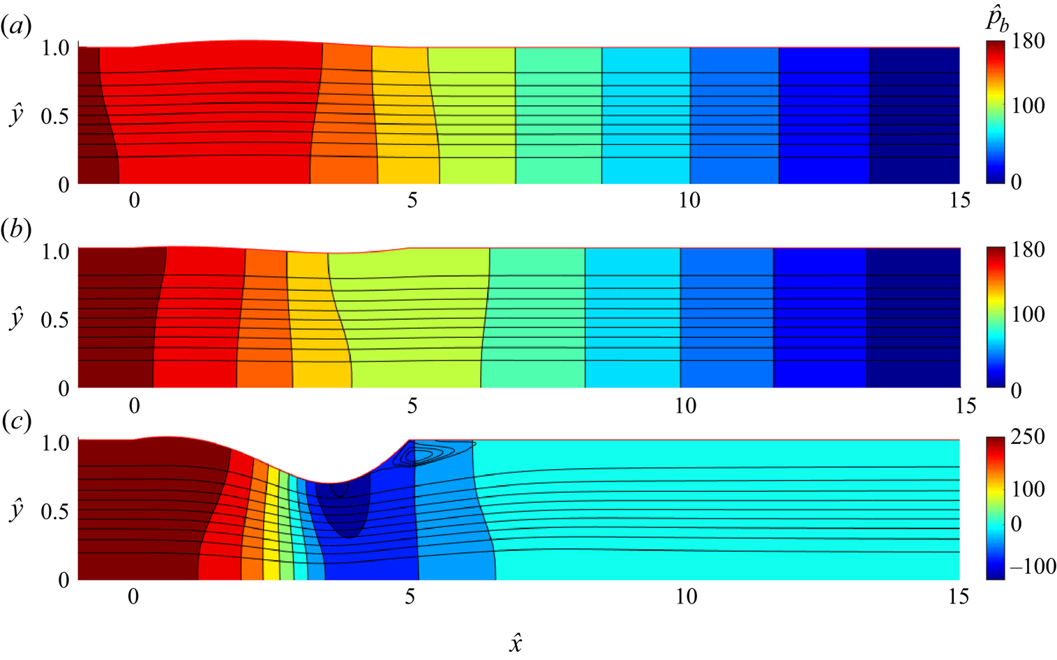
Figure 5. Streamlines and pressure contours for three branches of steady solutions for fixed Reynolds number ( $Re=500$) and fixed external pressure $\hat {p}_{ext}=1.52$: (a) the upper branch (branch I); (b) the intermediate branch (branch II); (c) the lower branch (branch III). Here, ${\hat {T}}_0=10$, ${\hat {e}}=0.01$ and ${\hat {\rho }}=0$.
3.2. Transition from the upper branch limit point
As the external pressure increases beyond the upper branch limit point the system abruptly transitions to the lower branch steady state. This transition is explored in figure 6, where we plot the unsteady evolution of the system from the upper branch limit point when the external pressure is instantaneously increased. In particular, we consider an unsteady simulation from the upper branch limit point at  $R=500$ for ${\hat {T}}_0=10$, displacing the external pressure from $\hat {p}_{ext}=1.52$ to $\hat {p}_{ext}=1.54$ (marked with a cross in figure 8). Over time the channel wall collapses monotonically toward the lower branch steady state (figure 6a). Initially, the rate of collapse is slow and the flow is laminar (figure 6b), but as the channel becomes increasingly constricted the rate of collapse increases and boundary layer separation takes place (figure 6c), where a re-circulation region becomes evident close to the downstream outlet of the compliant segment of the channel (figure 6d), creating a region of much lower pressure (figure 6e). A movie showing the entire transition is provided in the online supplementary material available at https://doi.org/10.1017/jfm.2021.1131.

Figure 6. Unsteady transition from the upper branch limit point to the lower steady branch for a thin wall ( ${\hat {e}}=0.01$) with no wall inertia ( ${\hat {\rho }}=0$): (a) time trace of the minimal channel width ( ${\hat {h}}_{min}$); streamlines and pressure colour map of the channel close to the outlet of the compliant segment at four selected times: (b) $t=215.0$; (c) $t=230.0$; (d) $t=245.0$; (e) $t=260.0$. The time points plotted in (b–e) are marked in panel (a). Here, $\hat {p}_e=1.54$, $Re=500$ and ${\hat {T}}_0=10$..
There is an interesting analogy between these observations and those reported for swirling flows in pipes (see for e.g. Lopez Reference Lopez1994; Herrada, Pérez-Saborid & Barrero Reference Herrada, Pérez-Saborid and Barrero2003), where fluid flows with a significant azimuthal velocity component through a rigid circular tube with an axisymmetric (fixed) sinusoidal indentation over a finite length. In this analogy the indentation of the pipe mirrors the collapse of the compliant segment of the channel, while the azimuthal fluid velocity component (and to some extent the compressibility of the fluid) extracts energy from the mean flow in a similar way to the compliance of the elastic wall. These swirling flows exhibit multiple (stable) steady solutions for a given set of parameters (when the Reynolds number is larger than a critical one) and the steady solutions can be described using bifurcation diagrams with three branches of steady solutions and two limit points, analogous to those presented in figure 4; this behaviour was recently termed ‘double hysteresis’ (Shtern Reference Shtern2018). These swirling flows also exhibit an unsteady transition from a nearly columnar flow to a recirculating flow when the swirling parameter is larger than a critical value (vortex breakdown), analogous to the spontaneous collapse of the channel we observe as the external pressure increases above the critical value ( $\hat {p}_{ext1}$). In the former case, centrifugal forces generate an adverse axial pressure gradient that induces a recirculating flow, whereas the channel collapse generates an adverse pressure gradient that drives detachment of the boundary layer adjacent to the flexible wall. The flow structures in figures 6–9 of Herrada et al. (Reference Herrada, Pérez-Saborid and Barrero2003) are reminiscent of the transition observed in figure 6, where in both cases the vortex breakdown occurs just downstream of the point of greatest indentation. The only significant difference comes in the cross-stream location of vortex shedding: the symmetry of the cylindrical geometry in the swirling flows results in vortex shedding near the axis of the tube, while in the collapsible channel the vortex shedding occurs near the flexible wall.
3.3. Linear stability results
Having computed the steady configurations of the system, we now analyse the temporal linear stability of the three different steady solution branches depicted in figure 4. For this large value of pre-tension ( ${\hat {T}}_0=10$) we find that the steady solutions along the section of the upper branch tested are globally stable to time-dependent perturbations (all the eigenvalues have $\omega _i<0$) for all external pressures greater than the outlet pressure (i.e. ${\hat {p}}_{ext}\geqslant 0$), while the solutions along the intermediate branch are always unstable (at least one eigenvalue has $\omega _i>0$ with $\omega _r=0$). Figure 7 illustrates the stability of the lower steady branch, showing the eigenvalue spectrum of the frequency $\omega$ for several values of the external pressure, ${\hat {p}}_{ext}$. In this case (and in figure 11 below) we focus only on the most unstable eigenvalues, illustrating those with $\omega _i>-0.5.$ We find that the lower branch is stable for sufficiently small external pressure, becoming globally unstable via a Hopf bifurcation when the external pressure exceeds a critical value, $\hat {p}_{ext}^\ast \approx 1.752$ (i.e. a pair of complex conjugate eigenvalues cross the real axis with non-zero $\omega _r$). At this critical point, the corresponding steady state is shown in figure 7(b), where it is inflated at the upstream end and collapsed at the downstream end (termed mode-2). The corresponding eigenfunction of the wall profile for the neutrally stable mode is shown in figure 7(c), which has two extrema (mode-2). We label the oscillatory modes associated with the lower branch with lower case Roman numerals (i), (ii), (iii) … in the order of increasing frequency, which is generally the order they become unstable as the external pressure increases, and so this primary instability is denoted mode-(i). These stability predictions agree well with the results presented by Heil (Reference Heil2004), where his figure 5 shows that the flow becomes unsteady and exhibits self-excited oscillations for $\hat {p}_{ext}=2.5$, well inside our unstable regime. These results are also qualitatively similar to the predictions of the one-dimensional model of Stewart (Reference Stewart2017), who showed that his lower branch of steady solutions becomes unstable to a mode-2 oscillation as the primary global instability of the system as the external pressure increases.

Figure 7. Stability of the lower steady branch to time-dependent perturbations for fixed Reynolds number ( $Re=500$) and fixed pre-tension ( ${\hat {T}}_0=10$): (a) five eigenvalue spectra in the $\omega$-plane for increasing values of ${\hat {p}}_{ext}$; (b) profile of the lower surface of the steady wall at neutral stability ( ${\hat {p}}_{ext} \approx 1.752$); (c) real and imaginary parts of the wall profile eigenfunction at neutral stability ( ${\hat {p}}_{ext} \approx 1.752$). Here, ${\hat {e}}=0.01$ and ${\hat {\rho }}=0$.
We overview the parameter space in figure 8 to summarise the regions of interest. We illustrate the region with multiple steady solutions by tracing the value of the external pressure at the limit points of the upper and lower steady branches ( $\hat {p}_{ext1}$ and $\hat {p}_{ext2}$, analogous to those found in figure 4) as a function of the Reynolds number; similar to Stewart (Reference Stewart2017), we find that this region with multiple steady states exists for Reynolds numbers greater than a threshold ( $Re>Re_{cusp} \approx 330$). We further plot the critical external pressure for the onset of oscillatory instability, $\hat {p}_{ext}^\ast$, as a function of the Reynolds number, finding that for the range of Reynolds numbers explored here the neutral stability curve lies entirely within the range where there is a unique steady solution along the lower steady branch, so $\hat {p}_{ext}^\ast >\hat {p}_{ext1}$. Note that we observe no instability of the upper steady branch for this choice of the wall pre-tension ( ${\hat {T}}_0=10$) across the range $0\leqslant {\hat {p}}_{ext} \leqslant {\hat {p}}_{ext1}$. It emerges below that this branch only becomes unstable for ${\hat {p}}_{ext} <0$ for this value of ${\hat {T}}_0$, which is not considered here. For large Reynolds number we might expect the neutral stability curve to enter the region of parameter space with multiple steady states (in a similar manner to Stewart Reference Stewart2017), but this possibility is discussed in more detail below.

Figure 8. Overview of the critical conditions for self-excited oscillations for pre-tension  ${\hat {T}}_0=10$, plotting the critical external pressure for instability as a function of the Reynolds number. The cross symbol indicates the point in parameter space which corresponds to the unsteady simulation shown in figure 6. Here, ${\hat {e}}=0.01$, ${\hat {\rho }}=0$.
3.4. The influence of the pre-tension in the solid
When the pre-tension of the elastic wall is reduced, we observe a decrease in the critical Reynolds number beyond which multiple steady flows exist, and the steady state bifurcation diagram and neutral stability curves become more complicated. To illustrate this complexity, in figure 9 we characterise the multiplicity of steady solutions that exist for a lower value of the pre-tension ( $\hat {T}_0=5$) while holding the Reynolds number fixed ( $Re=500$), plotting the minimal ( ${\hat {h}}_{min}$) and maximal ( ${\hat {h}}_{max}$) widths of the steady channel as a function of the external pressure, for the upper and lower branches of steady solutions, obtained following the same procedure as § 3.1. Similar to the case we considered in figure 4 ( $\hat {T}_0=10$), when the external pressure increases beyond a certain value, ${\hat {p}}_{ext}=\hat {p}_{ext1}$, there is a jump from a solution on the upper branch to a solution on the lower branch (where the channel becomes much more collapsed). In the same way, as we decrease the external pressure along the lower branch below a certain value, ${\hat {p}}_{ext}=\hat {p}_{ext2}$, there is a jump back to the upper branch.

Figure 9. Nonlinear steady solutions of the model for fixed Reynolds number ( $Re=500$) and pre-tension ( ${\hat {T}}_0=5$), showing the maximal and minimal channel widths as a function of the external pressure ${\hat {p}}_e$. Here, ${\hat {e}}=0.01$ and ${\hat {\rho }}=0$.
To overview these steady solutions across the parameter space, in figure 10 we plot the external pressure at the limit points of the steady solutions ( $\hat {p}_{ext1}$ and $\hat {p}_{ext2}$) as a function of the Reynolds number for a lower value of the pre-tension ( ${\hat {T}}_0=5$), where we find that the critical Reynolds number for multi-valued solutions has reduced ( $Re_{cusp} \approx 275$ in this case). To further illustrate the stability of these steady solutions, in figure 10 we also trace the critical external pressure for the onset of instability as a function of the Reynolds number, finding again that the lower branch of steady solutions (branch III) becomes unstable for external pressures greater than a critical value, $\hat {p}_{ext}^\ast$, and is stable otherwise (figure 10). This observation is similar to our observation for large pre-tension ( $\hat {T}_0=10$), with the only difference that now the loss of stability is closer to the region of multiplicity of steady solutions, with the two bounding curves almost overlapping for the largest Reynolds numbers considered. Tracing these curves to larger Reynolds numbers is an interesting direction of future work, where we might expect the neutral stability curve and the trace of the lower branch limit point to eventually intersect. Such an intersection was previously observed by Stewart (Reference Stewart2017), where the Hopf bifurcation (associated with the oscillation) and the saddle node bifurcation (associated with the steady solutions) interact in a co-dimension 2 bifurcation, suggesting a nearby homoclinic orbit (Glendinning Reference Glendinning1994).

Figure 10. Overview of the critical conditions for self-excited oscillations for lower pre-tension  ${\hat {T}}_0=5$, plotting the critical external pressure for instability as a function of the Reynolds number. The plus symbol indicates the point in parameter space which corresponds to the nonlinear portrait of the upper branch instability shown in figure 12. Here, ${\hat {e}}=0.01$, ${\hat {\rho }}=0$.
However, for this lower value of the pre-tension we also observe that steady solutions along the upper branch (branch I in figure 9) also become temporally unstable for external pressures below a critical value, denoted  $\hat {p}_{extI}^*$, and are stable otherwise (see figure 10). This means that for $Re>Re_{cusp}$ there is only a narrow interval of external pressures compatible with a steady stable flow, focused around the region with multiple steady solutions. Instability of the upper branch of steady solutions has recently been noted by Wang et al. (Reference Wang, Luo and Stewart2021a) using a flexible wall modelled as a thin nonlinear beam, but in their case the region of instability is located within and directly adjacent to the region with multiple steady solutions (Wang et al. Reference Wang, Luo and Stewart2021b), in contrast to that noted here. The fully developed limit cycles also exhibit some significant differences (see § 3.5 below).
To further explore this upper branch instability for lower pre-tension ( $\hat {T}_0=5$) and fixed Reynolds number ( $Re=400$), in figure 11(a) we plot the corresponding eigenvalue spectra for several values of the external pressure, where a complex conjugate pair of eigenvalues cross into the upper half-plane for ${\hat {p}} < {\hat {p}}_{extI}^* \approx 1.12$ (Note that ${\hat {p}}_{ext}^* \approx 1.66$), consistent with a Hopf bifurcation. At neutral stability the steady configuration of the flexible wall is entirely inflated with a single hump (termed mode-1, see figure 11b), while the neutrally stable eigenfunction of the oscillating wall profile is mode-2 (figure 11c), similar to the instability of the lower branch. Note that the frequency of oscillation along the upper branch is generally larger than the corresponding instability along the lower branch. Given that this oscillation also has a mode-2 structure of the wall shape eigenfunction, we label modes associated with the upper branch using Roman letters (a),(b), $\ldots$ in order of increasing frequency, which is generally the order they become unstable as the Reynolds number increases. The primary oscillatory mode associated with the upper branch is therefore labelled mode-(a). It is interesting to note that the instability of the mode-1 steady state exhibits a mode-2 eigenfunction profile, presumably because the prescribed upstream flux suppresses modes that induce large volume changes in the flexible segment of the channel (such as the mode-1 oscillations observed with prescribed upstream pressure e.g. Jensen & Heil Reference Jensen and Heil2003; Stewart et al. Reference Stewart, Waters and Jensen2009, Reference Stewart, Heil, Waters and Jensen2010).

Figure 11. Exploration of the lower branch instability for lower pre-tension  $\hat {T}_0=5$: (a) five eigenvalue spectra in the $\omega$ plane for increasing external pressure; (b) steady wall profiles for the choice of external pressure where the system is neutrally stable; (c) real and imaginary parts of the corresponding eigenfunction of the wall profile at neutral stability. Here, ${\hat {e}}=0.01$ and ${\hat {\rho }}=0$.
The upper branch neutral stability point,  ${\hat {p}}^\ast _{extI}$, can be traced (by numerical continuation) to larger values of the wall pre-tension; we find that the critical external pressure must become negative to induce instability for ${\hat {T}}_0=10$, explaining why it was not observed in figures 7 and 8, where we restrict attention to external pressures larger than the channel outlet pressure ( ${\hat {p}}_{ext}>0$).
We note that the neutral stability curves associated with both the upper and lower steady branches trace close to the region with multiple steady solutions as the Reynolds number increases, suggesting this region plays a key role in the structure of the dynamical system. Stewart (Reference Stewart2017) showed that the limit point on the upper steady branch (traced by the blue curve in figures 8 and 10) asymptotes to the saddle node bifurcation point for steady solutions of the inviscid system as the Reynolds number increases. Indeed, both Xu et al. (Reference Xu, Billingham and Jensen2013) and Stewart (Reference Stewart2017) identified the threshold where inviscid steady states emerge as an organising centre of the dynamical system, consistent with our observation. Conversely, the lower branch of steady solutions is entirely maintained by the fluid viscosity (Stewart Reference Stewart2017), and is thus absent in the inviscid limit.
3.5. Limit cycles of upper branch instability
Fully nonlinear simulations of self-excited oscillations growing from the lower branch of steady solutions have been widely reported elsewhere (e.g. Heil Reference Heil2004; Luo et al. Reference Luo, Cai, Li and Pedley2008). An instability of the upper branch of steady solutions was recently reported by Wang et al. (Reference Wang, Luo and Stewart2021a), who considered flow through a similar two-dimensional collapsible channel system modelling the flexible wall as a thin (nonlinear) beam with resistance to both bending and stretching (with no pre-stress), and the nonlinear limit cycles were explored using fully nonlinear simulations. However, the upper branch oscillations evident from the present model exhibit a significant difference in structure: for the oscillations reported by Wang the unstable region restabilises as the upper branch limit point is reached (Wang et al. Reference Wang, Luo and Stewart2021a) and remains confined to the neighbourhood of the region with multiple steady states (Wang et al. Reference Wang, Luo and Stewart2021b), whereas for the present model the system is stable in the neighbourhood of the upper branch limit point and instead the unstable region extends over a wide range of external pressures away from the region with multiple steady states (figure 10).
Given the difference in structure between our predictions and those of Wang et al. (Reference Wang, Luo and Stewart2021a), in figure 12 we examine the underlying dynamics of our upper branch oscillations using fully nonlinear simulations of our model (method described in § 2.5) at a point in parameter space within the upper branch neutral stability curve. In this case we choose  $Re=500$, $\hat {p}_{ext}=1$ and $\hat {T}_0=5$, marked with a plus inside the unstable region in figure 10. Initiating the simulation on the upper branch steady solution, numerical noise is enough to trigger an oscillatory instability evident in the time trace of the maximal channel width (see figure 12(a) with growth rate and frequency consistent with the global linear stability eigensolver), eventually saturating into a complicated nonlinear limit cycle (one period shown in figure 12b). A movie showing the flow field and vorticity over several periods of this limit cycle is provided in the online supplementary material.

Figure 12. The mechanism of upper branch instability for a thin hyperelastic wall ( ${\hat {e}}=0.01$) with no wall inertia ( ${\hat {\rho }}=0$): (a) the maximal channel width ${\hat {h}}_{max}$ as a function of time; (b) zoom-in over panel (a) over one period of oscillation; streamlines and pressure colour map of the channel close to the outlet of the compliant segment at six selected times over a period of oscillation including: (c) $t=1149.6$; (d) $t=1151.2$; (e) $t=1152.8$; (f) $t=1154$; (g) $t=1155$; (h) $t=1155.4$. The fully developed limit cycle of interest is enclosed in the red box in (a). The times corresponding to the snapshots in panels (c–h) are labelled in (b). Here, $Re=500$, $\hat {p}_{ext}=1$ and $\hat {T}_0=5$.
Over a period of this limit cycle the wall profile grows a single hump at the downstream end of the compliant segment (figure 12c); this hump propagates upstream reaching a global maximum (figure 12d) before being reflected back downstream again by the upstream rigid segment, where its amplitude subsequently decreases. As this hump propagates downstream a second hump appears at the downstream end of the compliant segment (figure 12e) which eventually dominates the first (figure 12f). However, these two humps do not coalesce but instead the  $x$-location of the maximum wall deflection changes discontinuously at the global minimum of ${\hat {h}}_{max}$ (figure 12(f), explaining the cusp in figure 12(b) at $t\approx 1138.2, 1145.5, 1152.8$). This second hump grows in amplitude, engulfing the remains of the first hump and shedding a low pressure vortex into the downstream rigid segment (figure 12g). This propagating vortex creates a so-called vorticity wave in the downstream rigid segment (particularly evident in figure 12c,g,h) while the large hump at the downstream end of the compliant segment drives a short region of channel collapse at the upstream end. As this vorticity wave propagates downstream, the single hump in the compliant segment propagates upstream, repeating the cycle. The nature of this oscillation exhibits many of the features of the nonlinear upper branch oscillations described by Wang et al. (Reference Wang, Luo and Stewart2021a), including the development of an upstream propagating hump. However, for their upper branch oscillations this hump is annihilated by the upstream rigid segment (not reflected) and the flow remains entirely laminar throughout, with no evidence of low pressure vortex shedding. However, the present model is restricted by the assumption of first-order elasticity, meaning that we cannot apply as many boundary conditions at each end of the beam as Wang et al. (Reference Wang, Luo and Stewart2021a) (who applied zero slope conditions at the end of the beam in addition to the clamped conditions).
These vorticity waves have previously been observed in channel flows with self-excited oscillations from a collapsed (lower branch) steady state (Luo & Pedley Reference Luo and Pedley1996; Luo et al. Reference Luo, Cai, Li and Pedley2008) or with prescribed (oscillatory) wall motion in one compartment (Stephanoff et al. Reference Stephanoff, Pedley, Lawrence and Secomb1983; Pedley & Stephanoff Reference Pedley and Stephanoff1985).
3.6. The influence of the wall thickness
In this subsection we analyse the influence of the dimensionless wall thickness,  $\hat {e}$, on the model predictions. We consider a particular case holding the pre-tension, external pressure and Reynolds number fixed ( $\hat {T}_0=5$, $\hat {p}_{ext}=2.98$ and $Re=50$). For these parameters, with wall thickness ${\hat {e}}=0.01$, the system has a unique steady wall shape where the external pressure is sufficiently large to collapse the channel wall ( ${\hat {h}}_{min}<1$). These parameters are chosen so that the system is just inside the unstable regime for lower branch oscillations ( $Re=50$ and ${\hat {T}}_0=5$ which has critical ${\hat {p}}^\ast _{ext}\approx 3.001$). In figure 13 we characterise how an increase in the wall thickness influences the underlying steady flow (figure 13a,b) and the critical conditions for the onset of lower branch oscillations (figure 13c,d). Considering the steady system first, figure 13(a) shows that the increase in wall thickness has little effect on the overall shape of the flexible wall for this value of Reynolds number; the channel becomes slightly less constricted as the wall thickness increases. Similarly, figure 13(b) shows that increasing wall thickness slightly reduces the maximal streamwise velocity through the constriction, $\hat {v}_{max}=\max _{x,y}({\hat {v}}_{1xb})$ (as expected by conservation of mass). However, the wall thickness plays a more significant role in determining the stability of these steady solutions. The increase of the wall thickness results in the initially unstable solution (for $\hat {e}=0.01$) becoming stable for a critical value of the wall thickness $\hat {e} \gtrsim 0.08$ (figure 13c), with a corresponding decrease in the frequency of oscillation (figure 13d).

Figure 13. The influence of the wall thickness on the steady and oscillatory solutions in the absence of wall inertia ( ${\hat {\rho }}=0$): (a) the minimal steady channel width ${\hat {h}}_{min}$ as a function of the wall thickness; (b) the maximal steady flow speed $v_{max}$ as a function of the wall thickness; (c) the growth rate of the primary oscillatory mode as a function of the wall thickness (mode-(i)); (d) the frequency of the primary oscillatory mode (mode-(i)) as a function of the wall thickness. Here, $\hat {T}_0=5$, $\hat {p}_{ext}=2.98$ and $Re=50$.
In order to quantify the effect of increasing the wall thickness on the stability of the system across the parameter space, in figure 14 we plot the critical external pressure for the onset of the primary oscillatory instability of the lower branch (mode-(i)), denoted as  $\hat {p}^*_{ext}$, as function of the Reynolds number for fixed pre-tension ( $\hat {T}_0=5$) and five different wall thicknesses ( ${\hat {e}}=0.01,0.2,0.4,{1,2}$). Note that we have limited our investigation to values of the Reynolds numbers smaller than the critical value required for multiple steady solutions ( $Re_{cusp}$), so the steady profile is unique. In the absence of wall inertia $(\hat {\rho }=0)$ the effect of the wall thickness on the critical conditions for instability remains weak for relatively thin walls ( ${\hat {e}}=0.01,0.2,0.4$): the steady flow remains almost unchanged (figure 13a,b) and there is only a mild stabilisation of the instability, characterised by an increase in the critical pressure needed to generate self-excited oscillations (figure 14). It emerges that the thickness of the wall must be of the order of the channel width (i.e. ${\hat {e}} \sim 1$) before there is any significant difference in the stability threshold. For example, for ${\hat {e}}=1$ and ${\hat {e}}=2$ the critical pressure for the onset of instability is more appreciably increased compared with ${\hat {e}}=0.01$ (figure 14a), while the oscillation frequency is decreased (figure 14b). Furthermore, for ${\hat {e}}=2$ the critical external pressure and oscillation frequency both saturate as the Reynolds number becomes large (figure 14). We show in § 3.7 below that changes to the stability of the system are even more prominent when we include wall inertia.

Figure 14. Overview of the critical conditions required for the onset of oscillations while changing the wall thickness, plotting the critical external pressure for the onset of oscillation  $\hat {p}_{ext}^*$ as a function of the Reynolds number for five different wall thicknesses ( ${\hat {e}}=0.01$, ${\hat {e}}=0.2$, ${\hat {e}}=0.4$, ${\hat {e}}=1$ and ${\hat {e}}=2$). Here, $\hat {T}_0=5$.
3.7. The influence of wall inertia
We now examine the influence of increasing wall inertia. It should be noted that the steady version of the full nonlinear equations (2.1) is independent of the wall inertia parameter  ${\hat {\rho }}$, and so all steady results are unchanged from those reported above. To study the additional influence of wall inertia on the onset of self-excited oscillations growing from the lower branch of static solutions, in figure 15 we trace the growth rate (figure 15a) and frequency (figure 15b) of the mode-(i) instability from figures 8 and 10 as a function of the wall inertia parameter $\hat {\rho }$; at neutral stability the eigenfunction profile of the oscillatory mode has two (three) extrema in the real (complex) part of the wall profile (figure 15c), meaning the number of extrema can change over a period of oscillation for these walls of finite thickness. For this choice of parameters the primary oscillatory mode of the lower branch (mode-(i)) is stable for ${\hat {\rho }}=0$, becoming unstable as the wall inertia parameter, ${\hat {\rho }}$, increases (figure 15a), while the corresponding oscillation frequency decreases (figure 15b). The perturbation growth rate for lower branch mode-(i) exhibits a local maximum at ${\hat {\rho }} \approx 10$ before asymptoting toward zero as the wall inertia parameter continues to increase. Hence, this mode of instability approaches stability with decreasing oscillation frequency as the wall gets heavier. However, as the wall inertia parameter increases a second mode of oscillation also becomes unstable at ${\hat {\rho }} \approx 12.72$ (figure 15a) with larger frequency than mode-(i) (figure 15b); we term this mode-(ii), which also has a perturbation wall profile with two extrema (figure 15d) albeit with a narrow boundary layer at the upstream end of the profile. Unlike the primary mode, the growth rate of this instability continues to increase as ${\hat {\rho }}$ increases for these parameter values, while the corresponding oscillation frequency again approaches zero (figure 15b). As the wall mass parameter becomes even larger, we eventually observe another mode becoming destabilised for ${\hat {\rho }} \approx 21.02$ with larger frequency (figure 15b) which we term mode-(iii), where the wall profile again exhibits two extrema with a narrow upstream boundary layer (see eigenfunction wall profile in figure 15e). Further increases in the wall inertia parameter destabilises mode-(iv) (figure 15a,b). Note that, in accordance with our naming convention, the oscillation frequency of each mode increases with increasing mode number (figure 15b). In summary, increasing the wall inertia parameter, for all other parameters held fixed, destabilises the primary global instability of the system, but also destabilises higher modes of instability.

Figure 15. The role of increasing wall inertia in the growth rate and frequency of self-excited oscillations for fixed wall thickness  ${\hat {e}}=0.2$: (a) the growth rate of the first four oscillatory modes as a function of the wall inertia parameter; (b) the corresponding frequency of the first four oscillatory modes as a function of the wall inertia parameter; spatial profiles of real and imaginary parts of the eigenfunctions at neutral stability for (c) mode-(i) ( ${\hat {\rho }} =0.631$); (d) mode-(ii) ( ${\hat {\rho }} =12.73$); (e) mode-(iii) ( ${\hat {\rho }} =21.02$). Here, $\hat {T}_0=5$, $\hat {p}_{ext}=2.98$ and $Re=50$.
In order to summarise the influence of increasing wall inertia across the parameter space, in figure 16 we plot the critical external pressure for the onset of lower branch oscillations,  ${\hat {p}}^\ast _{ext}$, as a function of the Reynolds number for constant wall thickness ( ${\hat {e}}=0.2$) and fixed pre-tension ( ${\hat {T}}_0=5$) for three different values of the wall inertia parameter ( ${\hat {\rho }}=0,10,50$). For small values of the wall inertia parameter ( ${\hat {\rho }}=0,10$) we find only mode-(i) across the section of parameter space considered (a direct continuation of mode-(i) identified in the absence of wall inertia); this mode becomes increasingly unstable as ${\hat {\rho }}$ increases (figure 16a), while the corresponding frequency of oscillation decreases (figure 16b). This observation is consistent with the work of Luo & Pedley (Reference Luo and Pedley1998), who found that increasing wall mass enlarges the unstable region of parameter space. However, consistent with figure 15, as the wall inertia parameter increases, additional (higher-frequency) modes of instability also arise in the system. In particular, we identify modes (i), (ii), (iii) and (iv), labelled in order of increasing frequency. In fact, it emerges that for ${\hat {\rho }}=50$, for the parameters investigated the mode-(ii) oscillation is more unstable than mode-(i) until $Re \approx 46$. Beyond this critical value mode-(iii) becomes the most unstable mode, while for even larger Reynolds numbers ( $Re \gtrsim 166$) there is another cross-over in parameter space and mode-(iv) becomes the most unstable mode. Note that the frequency of the oscillation increases with increasing mode number (figure 16b). These observations are again consistent with the predictions of Luo & Pedley (Reference Luo and Pedley1998), who found that a higher-frequency oscillatory mode eventually dominated the fundamental mode as the wall inertia parameter increased.

Figure 16. An overview of the critical conditions for the onset of instability for fixed wall thickness  ${\hat {e}}=0.2$ for three different values of the wall inertia parameter $\hat {\rho }=0,10,50$: (a) the critical external pressure for the onset of the four most unstable modes of the system (modes-(i) to (iv)) as a function of the Reynolds number; (b) the corresponding neutrally stable oscillation frequency of these four modes as a function of the Reynolds number. Here, ${\hat {T}}_0=5$.
Figure 16(a) also highlights that the structure of the neutral stability curve for mode-(iii) oscillations is somewhat different to the traces of mode-(i), (ii) and (iv), exhibiting a maximal Reynolds number and a two-branch structure analogous to the tongue structures seen in other collapsible channel systems (Luo et al. Reference Luo, Cai, Li and Pedley2008; Stewart Reference Stewart2017).
4. Discussion
In this paper we have developed a model for the flow of Newtonian fluid through a finite-length (asymmetric) flexible-walled channel, as a planar analogue of flow through a Starling resistor experiment. The flexible wall of the channel was assumed to be a pre-tensioned hyperelastic material of finite thickness, overcoming the limitation with more approximate models that require the elastic wall to be asymptotically thin (such as a membrane (e.g. Luo & Pedley Reference Luo and Pedley1996), a nonlinear beam (e.g. Luo et al. Reference Luo, Cai, Li and Pedley2008; Wang et al. Reference Wang, Luo and Stewart2021a) or an elastic shell (e.g. Heil Reference Heil2004)) and providing a much closer resemblance to the experiments where the tube walls are typically of the order of the tube radius (e.g. Bertram et al. Reference Bertram, Raymond and Pedley1990, Reference Bertram, Raymond and Pedley1991; Bertram & Castles Reference Bertram and Castles1999). It should be noted that in the limit of an asymptotically thin wall our hyperelastic model can be rationally reduced to either a membrane or an elastic shell depending on the assumptions. Flow through the channel is driven by a prescribed upstream flux against a prescribed downstream pressure, while the compliant segment of the channel is externally pressurised. This model is validated against previous predictions which approximated the wall using nonlinear shell theory (Heil Reference Heil2004), showing excellent agreement (figures 3, 4).
The numerical method used in this study is based on an arbitrary Lagrangian–Eulerian approach (Hirt, Amsden & Cook Reference Hirt, Amsden and Cook1974; Donea et al. Reference Donea, Huerta, Ponthot and Rodriguez-Ferran2004; Hron & Turek Reference Hron and Turek2006; Basting et al. Reference Basting, Quaini, Canic and Glowinski2017; Ryzhakov et al. Reference Ryzhakov, Rossi, Idelsohn and Onate2020), in that one can either move with the fluid (Lagrangian description) or view the flow from a fixed position (Eulerian description). The novelty of our method lies in the use of non-singular mappings between these two descriptions, in which all fields are solved simultaneously and which allow the method to be fully implicit. At the same time, we use high-order (fourth-order) finite differences or spectral Chebyshev collocation to discretise the transformed domains. Thus, while there are other such monolithic methods (e.g. Hron & Turek Reference Hron and Turek2006; Ryzhakov et al. Reference Ryzhakov, Rossi, Idelsohn and Onate2020), we are able to construct a stable method with high spatial accuracy. The numerical method used herein is well suited for solving other fluid–structure interaction problems (e.g. Bungartz & Schäfer Reference Bungartz and Schäfer2006) since it can handle large deformation of the solid with the help of these non-singular mappings; many standard implementations of fluid–structure interaction fail due to excessive mesh deformation.
The model predicts that at least one steady configuration of the system exists for all values of the parameters. For sufficiently large Reynolds numbers the system exhibits three co-existing steady states for a narrow range of the parameters. These states are connected by a pair of limit points, similar to earlier predictions using more approximate models (Luo & Pedley Reference Luo and Pedley2000; Stewart Reference Stewart2017) with two stable configurations (figures 4, 9): an upper branch (where the channel wall is entirely inflated) and a lower branch (where the channel wall is collapsed). Beyond the upper limit point the system transitions (dynamically) from the upper branch of steady solutions to the lower, where the wall profile becomes increasingly collapsed, the flow separates beyond the constriction and a low pressure vortex is shed into the downstream rigid segment (figure 6); such an observation has many similarities to swirling flows in pipes and open jets (Lopez Reference Lopez1994; Shtern & Hussain Reference Shtern and Hussain1996; Herrada et al. Reference Herrada, Pérez-Saborid and Barrero2003).
Similar to previous studies (Heil Reference Heil2004; Stewart Reference Stewart2017), we found an instability of the lower branch of steady solutions via a Hopf bifurcation when either the Reynolds number or the external pressure becomes sufficiently large (figures 8, 10). For the parameter values considered in this study we did not observe the neutral stability curve entering the region of multiple steady states. However, in line with observations of Stewart (Reference Stewart2017), we expect that the neutral stability curve will eventually terminate when it intersects the line of limit points along the lower branch of steady solutions.
However, our model also predicted that the upper branch of steady solutions could become unstable via a Hopf bifurcation to an entirely separate branch of mode-2 instabilities when the pre-tension is sufficiently low (figure 10). Note that an analogous instability of the upper branch has very recently been found in a model of Newtonian flow in a collapsible channel with a nonlinear elastic beam (Wang et al. Reference Wang, Luo and Stewart2021a). The fully developed limit cycle of our upper branch oscillations bears many similarities to those described by Wang et al. (Reference Wang, Luo and Stewart2021a), exhibiting a hump propagating upstream along the compliant segment and interacting with flow in the upstream rigid segment (figure 12); however, in our oscillations the hump is reflected by the upstream rigid segment and the flow sheds a low pressure vortex which drives a vorticity wave into the downstream rigid segment (Stephanoff et al. Reference Stephanoff, Pedley, Lawrence and Secomb1983; Pedley & Stephanoff Reference Pedley and Stephanoff1985).
Our new hyperelastic formulation provides an opportunity to investigate the role of wall thickness on the onset of instability. Previous studies of flow in thick-walled tubes or channels have been restricted to steady configurations (Marzo et al. Reference Marzo, Luo and Bertram2005; Zhang et al. Reference Zhang, Luo and Cai2018), while unsteady systems have typically considered asymptotically thin walls (Luo & Pedley Reference Luo and Pedley1996; Jensen & Heil Reference Jensen and Heil2003; Luo et al. Reference Luo, Cai, Li and Pedley2008). We found that, in the absence of wall inertia, increasing the wall thickness alone makes negligible difference to either the steady solutions (figure 13a,b) or the onset of oscillations (figures 13c,d, 14) until the wall thickness becomes comparable to the channel thickness (in this case the aspect ratio of the wall is relatively small  $h/L \lesssim 0.2$ and so thin-wall approximations are still appropriate). For even larger wall thicknesses the critical pressure for the onset of instability is significantly increased compared with the thin walls (figure 14), while the oscillation frequency is decreased (figure 14b). Furthermore, for the largest wall thickness considered the critical external pressure and oscillation frequency both saturate as the Reynolds number becomes large (figure 14).
The dimensionless parameter  $\hat {\rho }$ describes the strength of wall inertia compared with the internal elastic stress, but also represents an eigen-frequency of the elastic wall compared with the characteristic (inverse) time scale of the flow past the elastic wall. It is therefore important to characterise how these natural frequencies of wall vibration correlate to the other modes of self-excited oscillation of this system. Wall mass also plays an important role in physiological applications such as human phonation (Mittal, Erath & Plesniak Reference Mittal, Erath and Plesniak2013). We found that increasing the wall inertia parameter promotes the onset of self-excited oscillation by enlarging the unstable region of the primary (mode-2) global instability in the space spanned by Reynolds number and external pressure (figure 16); inertia-driven destabilisation was previously noted by Luo & Pedley (Reference Luo and Pedley1998). In addition, increasing the wall inertia parameter also destabilises higher-frequency modes of instability, which eventually dominate the primary global instability as the wall inertia parameter increases (figure 16), again consistent with the observations of Luo & Pedley (Reference Luo and Pedley1998). However, it turns out that the value of the parameter $\hat {\rho }$ is typically small for the silicone rubber tubes used in Starling resistor experiments; these tubes have been estimated to have a Young's modulus and Poisson ratio of $E=3.8$ MPa and $\nu =0.423$, respectively (Bertram Reference Bertram1987), resulting in a shear modulus of $\mu _2 = 1.335$ MPa (assuming an isotropic material). Silicone rubber also has an average density of $\rho _2=1240\ \textrm {kg}\ \textrm {m}^{-3}$. Starling resistor experiments in a tube with internal diameter 12 mm and a flow rate of the order of $60\ \textrm {ml}\ \textrm {s}^{-1}$ (Bertram & Tscherry Reference Bertram and Tscherry2006), exhibit a flow velocity of approximately $0.531\ \textrm {m}\ \textrm {s}^{-1}$. Flow of this velocity in a channel of thickness 1 mm corresponds to a flow rate per unit length in the out-of-plane direction of $q=5.31\times 10^{-4}\ \textrm {m}^2\ \textrm {s}^{-1}$. Using all this information, we estimate $\hat {\rho }\approx 2.62 \times 10^{-4}\ll 1$ for a compliant channel formed from silicone rubber.
Our hyperelastic formulation assumed first-order elasticity, with elastic stress proportional to the gradient of the strain energy function with respect to the strain tensor. We imposed lateral boundary conditions of no displacement along the face of the elastic solid in contact with the rigid wall. This approach cannot reproduce the resistance to bending of an elastic beam, since this would require strain gradient (second-order) elasticity, where the elastic stress has additional contributions due to the derivative of the strain energy function with respect to the strain gradient tensor; this approach would also require additional boundary conditions at the edges of the compliant segment. Indeed, Luo and coworkers considered a collapsible channel model where the (asymptotically thin) elastic wall exhibited resistance to both bending and stretching but no pre-tension, imposing clamped and zero slope conditions at each end of the flexible wall (Luo et al. Reference Luo, Cai, Li and Pedley2008; Wang et al. Reference Wang, Luo and Stewart2021a,Reference Wang, Luo and Stewartb). Their wall profiles accommodated this zero slope condition over very narrow boundary layers at each end of the compliant segment (see examples in Wang et al. Reference Wang, Luo and Stewart2021a). Furthermore, Wang et al. (Reference Wang, Luo and Stewart2021b) noted that increasing the resistance to bending of the beam narrowed the region of multiple steady states, and eventually suppressed the onset of self-excited oscillation. Similar to the present study, the model of Wang et al. (Reference Wang, Luo and Stewart2021a,Reference Wang, Luo and Stewartb) predicted self-excited oscillations growing from both the upper and lower branches of static solutions. However, their lower branch oscillations were typically of higher frequency and re-stabilised for sufficiently large external pressure (Wang et al. Reference Wang, Luo and Stewart2021b) (contrary to the present system where lower branch instability persisted as the external pressure increased, figures 8, 10). Both systems exhibited an upper branch instability of  $O(1)$ frequency, but in Wang et al. (Reference Wang, Luo and Stewart2021a,Reference Wang, Luo and Stewartb) the unstable zone remained localised to the neighbourhood of the upper branch limit point (contrary to the present system where the upper branch instability persisted to low external pressures, figure 10). However, it is unclear if these discrepancies are due to the differences in the constitutive assumptions between the two systems, or due to the absence of pre-tension in the work of Wang et al. (Reference Wang, Luo and Stewart2021a,Reference Wang, Luo and Stewartb). A more expansive comparison will be pursued in future work.
Supplementary movie
Supplementary movie is available at https://doi.org/10.1017/jfm.2021.1131.
Acknowledgements
Helpful discussions with Professor J.H. Snoeijer (University of Twente) are very gratefully acknowledged. We are very grateful to Professor M. Heil (University of Manchester) for providing the data used to plot figure 3(b).
Funding
M.A.H. and S.B.T. acknowledge funding from the Spanish Ministry of Economy, Industry and Competitiveness under Grants DPI2016-78887 and PID2019-108278RB and from the Junta de Andalucía under Grant P18-FR-3623. P.S.S. acknowledges funding from Engineering and Physical Sciences Research Council (UK) grants EP/P024270/1, EP/N014642/1 and EP/S030875/1.
Declaration of interests
The authors report no conflict of interest.
Supporting data
Supporting data for this paper can accessed at https://dx.doi.org/10.5525/gla.researchdata.1113.
Appendix. Convergence study of the numerical method
To illustrate the mesh independence of the numerical results we compute the real and imaginary components of the eigenvalue  ${\hat {\omega }}$ obtained from the global linear stability eigensolver for different discretisations of the domain, changing the number of mesh points $\xi _1$, $\xi _2$, $\chi _1$ and $\chi _2$ (listed in § 2.2). A typical example for an unstable point on the upper branch of steady solutions is provided in table 1, where we find that the real and imaginary parts of $\hat {\omega }$ show only negligible variations as the mesh is refined. The data listed in boldface correspond to the numerical mesh used in this work.
Table 1. Mesh sensitivity for an unstable case on the upper branch of steady solutions for a thin wall ( $\hat {e}=0.01$) with no wall inertia ( $\hat {\rho }=0$), listing the real and imaginary parts as a function of the discretisation parameters $\xi _1$, $\xi _2$, $\chi _1$ and $\chi _2$. The row listed in bold corresponds to the parameters used for the simulations in the main text. Here $\hat {T}_0=5$, $\hat {p}_{ext}=0.82$ and $Re=400$.


 Open access