


1. Introduction
Buoyancy and rotational forces drive and shape many large-scale flows in nature, such as swirling convection currents of conductive material in the Earth's outer core that generate the Earth's magnetic field (Cardin & Olson Reference Cardin and Olson1994; Glatzmaier et al. Reference Glatzmaier, Coe, Hongre and Roberts1999; Jones Reference Jones2000; Sarson Reference Sarson2000; Aubert, Gastine & Fournier Reference Aubert, Gastine and Fournier2017; Schaeffer et al. Reference Schaeffer, Jault, Nataf and Fournier2017; Guervilly, Cardin & Schaeffer Reference Guervilly, Cardin and Schaeffer2019), deep convection in the world's oceans (Marshall & Schott Reference Marshall and Schott1999; Gascard et al. Reference Gascard, Watson, Messias, Olsson, Johannessen and Simonsen2002; Wadhams et al. Reference Wadhams, Holfort, Hansen and Wilkinson2002; Budéus et al. Reference Budéus, Cisewski, Ronski, Dietrich and Weitere2004) and trade winds near the Earth's surface in the atmosphere (Hadley Reference Hadley1735). The influence of these forces is also observed beyond our own planet: as deep convection in the interior of gaseous planets (Busse & Carrigan Reference Busse and Carrigan1976; Busse Reference Busse1994; Yadav & Bloxham Reference Yadav and Bloxham2020) and zonal flows in their atmosphere (Ingersoll Reference Ingersoll1990; Sanchez-Lavega, Rojas & Sada Reference Sanchez-Lavega, Rojas and Sada2000; Porco et al. Reference Porco2003; Heimpel & Aurnou Reference Heimpel and Aurnou2007; Heimpel, Gastine & Wicht Reference Heimpel, Gastine and Wicht2016; Cabanes et al. Reference Cabanes, Aurnou, Favier and Le Bars2017), as well as in the convection zone of stars like our Sun (Miesch Reference Miesch2000; Cattaneo, Emonet & Weiss Reference Cattaneo, Emonet and Weiss2003; Balbus et al. Reference Balbus, Bonart, Latter and Weiss2009; Hindman, Featherstone & Julien Reference Hindman, Featherstone and Julien2020).
Understanding the dynamics of these geophysical and astrophysical flows is paramount, however, their sheer size, remoteness and complexity preclude their direct investigation. A relatively simple, but highly relevant framework to investigate these flows is provided by the problem of rotating Rayleigh–Bénard convection (RRBC), where a rotating fluid layer is heated from below and cooled from above. In this system, the Rayleigh number  ${{Ra}}$ parameterises the strength of the thermal forcing, the Ekman number $\mathit {Ek}$ (and, alternatively, the convective Rossby number ${{Ro_{C}}}$) measures the strength of rotation, and the Prandtl number ${Pr}$ involves the diffusive properties of the fluid. Large-scale flows are characterised by extreme values of these governing parameters. In the Earth's outer core, ${{Ra}}$ is estimated to be $\textit {O}({10^{20} - 10^{30}})$, $\mathit {Ek}\sim \textit {O}({10^{-15}})$ and ${Pr}\sim \textit {O}({10^{-2} - 10^{-1}})$. Such conditions are certainly unfeasible for present-day simulations and experiments, yet studies at moderate parameter values have made great strides towards understanding the flow phenomenology in RRBC – see Kunnen (Reference Kunnen2021) for a recent review. In particular, it has been observed that a plethora of convection states exists in the range between rapidly rotating and non-rotating convection. Specifically, the parameter space of RRBC is partitioned into several regimes where the flow manifests as: quasi-steady convection cells (Chandrasekhar Reference Chandrasekhar1961); convective Taylor columns (only at ${Pr}\gtrsim 2$) (Sakai Reference Sakai1997; Sprague et al. Reference Sprague, Julien, Knobloch and Werne2006; Grooms et al. Reference Grooms, Julien, Weiss and Knobloch2010; Kunnen, Clercx & Geurts Reference Kunnen, Clercx and Geurts2010; Julien et al. Reference Julien, Rubio, Grooms and Knobloch2012; King & Aurnou Reference King and Aurnou2012; Rajaei, Kunnen & Clercx Reference Rajaei, Kunnen and Clercx2017; Noto et al. Reference Noto, Tasaka, Yanagisawa and Murai2019; Chong et al. Reference Chong, Shi, Ding, Ding, Lu, Zhong and Xia2020; Shi et al. Reference Shi, Lu, Ding and Zhong2020), plumes (Sprague et al. Reference Sprague, Julien, Knobloch and Werne2006; Kunnen et al. Reference Kunnen, Clercx and Geurts2010; Julien et al. Reference Julien, Rubio, Grooms and Knobloch2012; Rajaei et al. Reference Rajaei, Kunnen and Clercx2017; Maffei et al. Reference Maffei, Krouss, Julien and Calkins2021); geostrophic turbulence (Sprague et al. Reference Sprague, Julien, Knobloch and Werne2006; Julien et al. Reference Julien, Rubio, Grooms and Knobloch2012; Maffei et al. Reference Maffei, Krouss, Julien and Calkins2021; Rubio et al. Reference Rubio, Julien, Knobloch and Weiss2014; Stellmach et al. Reference Stellmach, Lischper, Julien, Vasil, Cheng, Ribeiro, King and Aurnou2014); rotation-affected convection (Ecke & Niemela Reference Ecke and Niemela2014; Kunnen et al. Reference Kunnen, Ostilla-Mónico, van der Poel, Verzicco and Lohse2016); and non-rotating convection (Malkus Reference Malkus1954; Kraichnan Reference Kraichnan1962; Spiegel Reference Spiegel1971; Castaing et al. Reference Castaing, Gunaratne, Heslot, Kadanoff, Libchaber, Thomae, Wu, Zaleski and Zanetti1989; Ahlers, Grossmann & Lohse Reference Ahlers, Grossmann and Lohse2009; Lohse & Xia Reference Lohse and Xia2010). The cellular regime is typically found in the range $1 \lesssim {{Ra/Ra_c}} \lesssim 2$ ( ${{Ra}}_c\sim \mathit {Ek}^{-4/3}$ is the critical Rayleigh number for onset of convection), and consists of narrow quasi-steady cells with horizontal size $\ell _c\sim \mathit {Ek}^{1/3}$ (Chandrasekhar Reference Chandrasekhar1961). Columns manifest at larger ${{Ra/Ra_c}}$, and are surrounded by ‘shields’ of opposite vertical vorticity and opposite temperature fluctuation. With increasing ${{Ra/Ra_c}}$, the shields become weaker and the vortical columns interact with each other. As a result, their vertical coherence is affected, leading to the development of plumes. At larger ${{Ra/Ra_c}}$, the geostrophic turbulence regime manifests. The combination of turbulence and strong rotational constraint leads to a quasi-two-dimensional dynamics that enables the transfer of kinetic energy from small to large spatial scales. This upscale energy transfer can lead to the formation of large-scale vortices (LSVs). In the rotation-affected regime, no upscale energy transfer is present (Kunnen et al. Reference Kunnen, Ostilla-Mónico, van der Poel, Verzicco and Lohse2016) as rotational forces are no longer dominant, instead the turbulent flow is thought to be dominated by buoyancy. Finally, in the non-rotating convection regime, Coriolis forces have no dynamical effect.
Numerous investigations into the interplay amongst the forces governing RRBC have been primarily focussed on the determination of the most relevant forces in geophysical and astrophysical settings. These studies aim to determine the dominant force balance in these large-scale flows in order to estimate the characteristic flow velocity and characteristic length scale of the convective motions therein (Stevenson Reference Stevenson1979; Aubert et al. Reference Aubert, Brito, Nataf, Cardin and Masson2001; Christensen Reference Christensen2002; Aubert Reference Aubert2005; King & Buffett Reference King and Buffett2013; King, Stellmach & Buffett Reference King, Stellmach and Buffett2013; Aurnou et al. Reference Aurnou, Calkins, Cheng, Julien, King, Nieves, Soderlund and Stellmach2015; Gastine, Wicht & Aubert Reference Gastine, Wicht and Aubert2016; Guervilly et al. Reference Guervilly, Cardin and Schaeffer2019; Aurnou, Horn & Julien Reference Aurnou, Horn and Julien2020). However, the role of subdominant forces has not been addressed extensively. A complete view of the interplay between all forces is required to effectively characterise the flow and its transitional behaviours between regimes. In this study, we focus on fully understanding the force balance, from the leading contributors to the subdominant forces. Previous efforts have been made in this direction in the field of rotating magnetoconvection (Soderlund, King & Aurnou Reference Soderlund, King and Aurnou2012; Calkins et al. Reference Calkins, Julien, Tobias and Aurnou2015; Yadav et al. Reference Yadav, Gastine, Christensen, Wolk and Poppenhaeger2016; Aubert et al. Reference Aubert, Gastine and Fournier2017; Aubert Reference Aubert2019; Schwaiger, Gastine & Aubert Reference Schwaiger, Gastine and Aubert2021). Self-sustained convective dynamos in planetary systems operate in a rotationally constrained regime. There, a balance is thought to hold amongst the Coriolis, pressure gradient, buoyancy and Lorentz forces, also known as magneto–Archimedean–Coriolis (MAC) balance. Hence, many studies seek to determine the specific parameter values and length scales at which the contribution of viscous and inertial forces becomes negligible, and therefore a MAC balance is possible. In our simulations of non-magnetic, rotating convection in a horizontal plane fluid layer, we access both low-supercriticality flow regimes, where viscous effects are expected to be significant, and highly supercritical regimes, where we foresee an increased importance of inertial forces. Similar low- and high-supercriticality RRBC flows have been studied by means of asymptotically reduced equations (Sprague et al. Reference Sprague, Julien, Knobloch and Werne2006; Julien et al. Reference Julien, Rubio, Grooms and Knobloch2012; Plumley et al. Reference Plumley, Julien, Marti and Stellmach2016; Maffei et al. Reference Maffei, Krouss, Julien and Calkins2021), valid at  $\mathit {Ek},{{{Ro_{C}}}} \rightarrow 0$. In these studies the geostrophic regimes (cells, columns, plumes and geostrophic turbulence with LSVs) are charted. Here, we assess the force balance of the full Navier–Stokes equations in these regimes and at larger ${{Ra/Ra_c}}$ in the rotation-affected regime. We identify flow transitions as distinct changes in the dominant or subdominant force balance, leading to a natural identification of each regime. We mainly consider the case of no-slip walls. This type of boundary condition is especially relevant to realistic settings such as laboratory experiments and large-scale flows in nature.
The remainder of this paper is structured as follows. Section 2 introduces the equations of motion of RRBC, as well as the equations used to calculate the force magnitudes. In § 3, we describe the numerical method and tabulate the parameter values for the simulations. In § 4.1 we present the flow structures observed for the explored parameter values. The midheight magnitude of the forces is discussed in § 4.2 as a function of the flow supercriticality. There, we also identify the characteristic force balance of the distinct flow regimes. The interplay amongst the forces in the region close to the no-slip walls is investigated in § 4.3. Finally, in § 5 we present our conclusions.
2. Governing equations and dimensionless parameters
We consider the buoyancy-driven flow between two parallel horizontal walls, with relative temperature difference  $\Delta T = T_{bottom} - T_{top}>0$, separated by a vertical distance $H$. The rotation vector $\varOmega \hat {\boldsymbol {z}}$ is parallel to the vertical unit vector $\hat {\boldsymbol {z}}$, whereas the gravitational acceleration is $\pmb {g}=-g\hat {\boldsymbol {z}}$. The flow is incompressible, and the kinematic viscosity, thermal diffusivity and thermal expansion coefficient of the fluid are $\nu$, $\kappa$ and $\alpha$, respectively. We model rotating thermal convection by using the non-dimensional Navier–Stokes and heat equations in the Boussinesq approximation (Chandrasekhar Reference Chandrasekhar1961),
 $$\begin{gather} \frac{\partial \pmb{u}}{\partial t} ={-} ( \pmb{u} \pmb{\cdot} \pmb{\nabla} ) \pmb{u} - \frac{1}{{{Ro_{C}}}} \hat{\boldsymbol{z}} \times \pmb{u} - \pmb{\nabla} p + \sqrt{\frac{Pr}{Ra}} \nabla^{2} \pmb{u} + \theta \hat{\boldsymbol{z}} , \end{gather}$$
 $$\begin{gather}\frac{\partial \theta}{\partial t} + ( \pmb{u} \pmb{\cdot} \pmb{\nabla} ) \theta = \frac{1}{\sqrt{RaPr}} \nabla^{2} \theta , \end{gather}$$
with the incompressibility constraint
 \begin{equation} \pmb{\nabla} \boldsymbol{\cdot} \pmb{u} = 0 . \end{equation}
We use  $H$,
$H$,  $\Delta T$ and the characteristic ‘free-fall’ velocity scale $U_{{\scriptsize ff}}=\sqrt {g \alpha \Delta T H}$ to obtain the non-dimensional velocity $\pmb {u}$, temperature $\theta$, pressure $p$ and time $t$. Equations (2.1) and (2.2) involve three non-dimensional parameters,
 \begin{equation} {{Ra}} = \frac{g\alpha\Delta T H^{3} }{\nu \kappa}, \quad {Pr} = \frac{\nu}{\kappa}, \quad {{Ro_{C}}} = \frac{\sqrt{g\alpha\Delta T / H}}{2 \varOmega} , \end{equation}
where  ${{Ra}}$ is the Rayleigh number, ${Pr}$ is the Prandtl number and the convective Rossby number ${{Ro_{C}}}$ parameterises the (inverse) strength of rotation. Alternatively, the strength of rotation can be quantified by means of the Ekman number $\mathit {Ek} = \nu / (2 \varOmega H^{2})$, which provides the ratio of viscous to Coriolis forces. A convenient relation between the various dimensionless parameters is ${{Ro_{C}}} = \mathit {Ek} ({{Ra}} / {Pr})^{1/2}$.
The velocity field in (2.1)–(2.3) must fulfil the impenetrable no-slip boundary condition  $\pmb {u}=\pmb {0}$ at the walls. Cases with stress-free boundary conditions comply with $\partial u/\partial z = \partial v/\partial z = 0$ and $w=0$ at the walls. The temperature field must meet the conducting boundary condition $\theta =1$ at the bottom and $\theta =0$ at the top.
Rotation, contrary to convection, has a stabilising effect on the flow. Therefore, at low values of the Rayleigh number and sufficiently strong rotation (low  $\mathit {Ek}$ and ${{Ro_{C}}}$), no convective motions take place, and the heat transfer from bottom to top boundary is exclusively due to conduction. In a laterally unbounded fluid layer subject to rapid rotation ( $\mathit {Ek} \lesssim 10^{-3}$), the critical Rayleigh number $Ra_c$ for the onset of convection is given by
 \begin{equation} Ra_c =\begin{cases}
17.4(\mathit{Ek} / {Pr} )^{{-}4/3} & \text{for }
{Pr}<0.68,\\[2pt] 8.7\mathit{Ek}^{{-}4/3} & \text{for } {Pr} \ge
0.68 \end{cases} \end{equation}
\begin{equation} Ra_c =\begin{cases}
17.4(\mathit{Ek} / {Pr} )^{{-}4/3} & \text{for }
{Pr}<0.68,\\[2pt] 8.7\mathit{Ek}^{{-}4/3} & \text{for } {Pr} \ge
0.68 \end{cases} \end{equation}
(Chandrasekhar Reference Chandrasekhar1961; Aurnou et al. Reference Aurnou, Bertin, Grannan, Horn and Vogt2018). Past this threshold, bulk convection starts in the form of oscillatory structures for  ${Pr}<0.68$, or steady cells for ${Pr} \ge 0.68$. Based on this critical value we define supercriticality as ${{Ra}}/Ra_c$, where $Ra_c$ takes either definition in (2.5) depending on the Prandtl number of a given study case. Our results are presented as a function of ${{Ra/Ra_c}}$ throughout this work.
The characteristic horizontal length scale  $\ell _c$ (normalised by the domain height $H$) of the onset structures is given by
 \begin{equation} \ell_c =\begin{cases} 2.4 (\mathit{Ek} / {Pr} )^{1/3} & \text{for } {Pr}<0.68,\\[2pt] 2.4 \mathit{Ek}^{1/3} & \text{for } {Pr} \ge 0.68 \end{cases} \end{equation}
(Chandrasekhar Reference Chandrasekhar1961; Heard & Veronis Reference Heard and Veronis1971; Julien et al. Reference Julien, Aurnou, Calkins, Knobloch, Marti, Stellmach and Vasil2016), again, valid for a laterally unbounded layer of fluid and rapid rotation ( $\mathit {Ek} \lesssim 10^{-3}$).
From (2.1), the governing forces of RRBC (the inertial, Coriolis, pressure gradient, viscous and buoyancy forces) are, in dimensionless form,
 \begin{equation} \left.\begin{array}{c@{}}
\displaystyle\pmb{F}_I
={-}{{(\boldsymbol{u}\boldsymbol{\cdot}\boldsymbol{\nabla})\boldsymbol{u}}}
, \quad \pmb{F}_C
={-}{\dfrac{1}{{Ro_{C}}}\hat{\boldsymbol{z}}\times
\boldsymbol{u}}, \quad \pmb{F}_P ={-}{\boldsymbol{\nabla}
p},\\[8pt] \displaystyle\pmb{F}_V =
{\sqrt{\dfrac{Pr}{{Ra}}}\nabla^2 \boldsymbol{u}}, \quad
\pmb{F}_B = {{\theta\hat{\boldsymbol{z}}}} ,
\end{array}\right\} \end{equation}
\begin{equation} \left.\begin{array}{c@{}}
\displaystyle\pmb{F}_I
={-}{{(\boldsymbol{u}\boldsymbol{\cdot}\boldsymbol{\nabla})\boldsymbol{u}}}
, \quad \pmb{F}_C
={-}{\dfrac{1}{{Ro_{C}}}\hat{\boldsymbol{z}}\times
\boldsymbol{u}}, \quad \pmb{F}_P ={-}{\boldsymbol{\nabla}
p},\\[8pt] \displaystyle\pmb{F}_V =
{\sqrt{\dfrac{Pr}{{Ra}}}\nabla^2 \boldsymbol{u}}, \quad
\pmb{F}_B = {{\theta\hat{\boldsymbol{z}}}} ,
\end{array}\right\} \end{equation}
respectively. Thus, the geostrophic balance can be written as  $\pmb {F}_C=-\pmb {F}_P$. To estimate the magnitude of these forces, we follow a procedure inspired by that used by Aubert et al. (Reference Aubert, Gastine and Fournier2017), Yadav et al. (Reference Yadav, Gastine, Christensen, Wolk and Poppenhaeger2016), Aubert (Reference Aubert2019), Schwaiger, Gastine & Aubert (Reference Schwaiger, Gastine and Aubert2019) and Maffei et al. (Reference Maffei, Krouss, Julien and Calkins2021). We compute the plane-averaged root mean square (r.m.s.) of each force. That is, for a given force $\pmb {F}(\boldsymbol {x})$ with $x$-,
$x$-,  $y$- and $z$-components $F_x(\boldsymbol {x})$, $F_y(\boldsymbol {x})$ and $F_z(\boldsymbol {x})$, its r.m.s. value is here defined as
 \begin{equation} F(z)=\sqrt{\langle (F_x-\langle F_x \rangle)^{2} + (F_y-\langle F_y \rangle)^{2} + (F_z-\langle F_z \rangle)^{2} \rangle} , \end{equation}
where  $\langle \cdot \rangle$ denotes averaging along the horizontal directions; therefore, $F$ is a function of the vertical coordinate $z$ only. In practice, on our laterally periodic domain, $\langle F_x \rangle \approx \langle F_y \rangle \approx \langle F_z \rangle \approx 0$ for the corresponding components of the inertial, Coriolis and viscous forces. For the pressure-gradient force and the buoyancy force, the deviations from the mean force components, e.g. $F_x-\langle F_x \rangle$, are considered in order to disregard the underlying mean vertical profiles of pressure and temperature; these profiles describe the mean hydrostatic balance in the system. Therefore, (2.8) enables the faithful calculation of the magnitude $|\pmb {F}(\boldsymbol {x})|$ of the governing forces contributing to the dynamics in RRBC. We note that the plane-averaging procedure considers that the flow is statistically homogeneous in the horizontal directions. Hence, we are able to evaluate the spatial dependence of the force balance solely in terms of the vertical coordinate. The force components are calculated at each grid position on a horizontal cross-section. We consider a one single-time volume snapshot well within the statistically stationary state; for other snapshots within this state the results agree within 5 % on average.
3. Numerical set-up
Equations (2.1)–(2.3) are solved using direct numerical simulation on a horizontally periodic Cartesian domain. The simulations are performed using two codes, both based on the principal set-up of the Verzicco code (Verzicco & Orlandi Reference Verzicco and Orlandi1996; Ostilla-Mónico et al. Reference Ostilla-Mónico, Yang, van der Poel, Lohse and Verzicco2015). The codes differ in their approach to resolve the temperature field: one resolves both velocity and temperature on a single grid, and the other resolves temperature on a different grid than that for velocity. This distinction is due to the diffusive properties of the fluid, parameterised by the Prandtl number. Recall that the smallest active length scales for velocity and temperature fluctuations, i.e. the Kolmogorov length scale  $\eta _K$ and the Batchelor length scale $\eta _B$, respectively, are related by $\eta _B=\eta _K{Pr}^{-1/2}$. Hence, $\eta _K<\eta _B$ for fluids with low Prandtl number ${Pr}<1$, whereas $\eta _B$ is smaller for high ${Pr}>1$. The latter property is exploited by the multiple-grid code in that it uses a finer grid to resolve the smaller temperature features, and a coarser grid to resolve the three-component velocity field. We use the single-grid code to simulate low- $Pr$ fluid flows, and the multiple-grid code for cases at high $Pr$. A complete list of the cases investigated can be found in table 1.
Table 1. Parameters for the simulations: Prandtl number  ${Pr}$; Ekman number $\mathit {Ek}$; Rayleigh number ${{Ra}}$; convective Rossby number ${{Ro_{C}}}$; supercriticality ${{Ra/Ra_c}}$; and domain aspect ratio $\varGamma$. The slight difference in $Pr$ between the $Pr\approx 5$ simulation series is for comparison with (ongoing) experiments in our group (Cheng et al. Reference Cheng, Aurnou, Julien and Kunnen2018, Reference Cheng, Madonia, Aguirre Guzmán and Kunnen2020). The Nusselt number ${Nu}$ is the mean of five ways of measuring the convective heat transfer (discussed in the text). These measurements converge within 5 % of the mean value ${Nu}$. The number of grid points to resolve the velocity field are $N_x$ and $N_z$ ( $N_y=N_x$), and the refinement factors for temperature $m_x$ and $m_z$ ( $m_y=m_x$). The last column indicates the observed flow morphology: convective cells (C); convective Taylor columns (T); plumes (P); LSVs; or rotation-affected convection (RA). All cases are simulated with no-slip walls. Some cases, denoted with the superscript ‘ $^{*}$’, are also independently simulated with stress-free boundaries. In the case denoted with ‘ $^{{\dagger} }$’ there are signs of upscale energy transfer, but no LSVs develop.

The single-grid code is a Cartesian adaptation of the original Verzicco cylinder convection code (Verzicco & Orlandi Reference Verzicco and Orlandi1996; Verzicco & Camussi Reference Verzicco and Camussi2003), where the governing equations are discretised by second-order finite-differences with dynamic time stepping for the time advancement. The multiple-grid code, which also used this numerical scheme (Ostilla-Mónico et al. Reference Ostilla-Mónico, Yang, van der Poel, Lohse and Verzicco2015), allows refinement of the grid for temperature in the  $x$-,
$x$-,  $y$- and $z$-directions independently, through the refinement factors $m_x$, $m_y$ and $m_z$. In our domains the lateral sides are of equal length, thus $m_y=m_x$. The refinement is relative to the grid for velocity, thus $m_x$, $m_y$ and $m_z$ are selected based on the ratio $\eta _K/\eta _B={Pr}^{1/2}$, and making sure to allocate an appropriate number of grid points within the thermal boundary layers (discussed below).
For all simulations the domain aspect ratio  $\varGamma =W/H$ allows a sufficiently large sampling of convective structures, whose characteristic length scale $\ell _c$ is given by (2.6). This procedure ensures the convergence of spatially averaged statistics. At low $Pr$, the domain size is $10\ell _c\times 10\ell _c\times 1$ (normalised by the domain height $H$). The multiple-grid strategy allows us to simulate high- $Pr$ fluid flows much more efficiently compared with the single-grid code, thus facilitating the exploration of wider domains of size $20\ell _c\times 20\ell _c\times 1$ at high $Pr$.
$Pr$.
Both codes use a grid with uniform horizontal spacing and non-uniform vertical distribution. In this way, a larger density of grid points can be placed near the walls to resolve the thin boundary layers. We verify, a posteriori, that a minimum of 11 grid points is allocated within the thinner (kinetic or thermal) boundary layer, which is enough to appropriately resolve it.
To validate the bulk resolution, we compare the grid spacing with the Kolmogorov and Batchelor length scales,  $\eta _K$ and $\eta _B$. We find that for low- ${Pr}$ runs the bulk resolution is $\Delta z_u/\eta _K < 3$ and $\Delta z_\theta /\eta _B < 1$, where $\Delta z_u$ and $\Delta z_\theta$ are the vertical grid spacing for the velocity and temperature field, respectively. For simulations at high $Pr$, we find $\Delta z_u/\eta _K < 3$ and $\Delta z_\theta /\eta _B < 3.7$. For all cases the horizontal grid spacing is smaller than the vertical one.
To further confirm the adequacy of the grid, we compute the time-averaged convective heat transfer  ${Nu}$ in five different ways: as the plane-averaged wall-normal temperature gradient at the bottom and at the top wall; as the volume-averaged convective flux; and the last two are based on exact relations for the dissipation rate of kinetic energy and thermal variance (Shraiman & Siggia Reference Shraiman and Siggia1990). For all cases the maximum difference between a given ${Nu}$ and the mean of all ${Nu}$ converges to better than a few per cent. This convergence is achieved over simulation times of the order of $10^{2}$ convective time units. The mean ${Nu}$ for all simulation cases is reported in table 1.
4. Results
4.1. Flow structures
Our RRBC survey spans a wide range of parameter values that jointly resolve over three decades of supercriticality  ${{Ra/Ra_c}}$. This allows the exploration of distinct flow regimes: C, T, P, LSVs and RA. In our set of simulations at
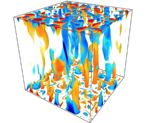
  ${Pr}\approx 5$, we observe the regimes of cells, convective Taylor columns, plumes and large-scale vortices. We present visualisations of the temperature fluctuations in these regimes in figures 1(a) to 1(d), respectively. The large-scale vortices in figure 1(d) are better visualised in terms of the horizontal kinetic energy of the flow, as we show in figure 2(a). All of our simulation cases at ${Pr}=100$ lie within the plumes regime; we show two example cases in figures 1(e) and 1(f). For the exploration of highly supercritical regimes we make use of a lower Prandtl number, ${Pr}=0.1$. The reason is that sufficiently small values of ${Pr}$ (i.e. smaller than 0.68, see (2.5)) act to decrease the critical Rayleigh number for onset of convection $Ra_c$. Thus, for a given value of ${{Ra}}$ and $\mathit {Ek}$, low- ${Pr}$ fluid flows can achieve a larger degree of supercriticality than those at high ${Pr}$. In other words, inertial effects are amplified in low- ${Pr}$ fluids (Julien et al. Reference Julien, Rubio, Grooms and Knobloch2012; Aurnou et al. Reference Aurnou, Bertin, Grannan, Horn and Vogt2018). At ${Pr}=0.1$ we also observe large-scale vortices and, at larger ${{Ra/Ra_c}}$, we identify rotation-affected convection – see figures 1(g) and 1(h), respectively. Just like at ${Pr}\approx 5$, the LSVs are more clearly visualised in terms of the horizontal kinetic energy of the flow – we show this in figure 2(b). In the rotation-affected regime, convection becomes more three-dimensional and, in the particular case displayed in figure 1(h), the large parcel of hot fluid (red patch at the top) and large parcel of cold fluid (blue patch) resemble a large overturning cell similar to that observed in non-rotating convection. However, in this case, the magnitude of the Coriolis force is still appreciable as we shall discuss in § 4.2. Finally, in order to discuss the observed flow regimes with increasing supercriticality, we present our results starting from simulations at ${Pr}\approx 5$ and $100$, and then at ${Pr}=0.1$.

Figure 1. Temperature fluctuations for selected cases in the observed flow regimes. In the captions, T stands for convective Taylor columns, LSVs for large-scale vortices, RA for rotation-affected convection,  $Pr$ is Prandtl number and ${{Ra/Ra_c}}$ is flow supercriticality. Owing to the low $\mathit {Ek}\sim 10^{-7}$ considered for all cases, the domain aspect ratio $\varGamma = W/H = \textit {O}({Ek^{1/3}})$ ( $W$ and $H$ are its width and height) is smaller than unity, i.e. the computational domains are narrower than they are tall. Thus, for clarity, the domains are stretched horizontally by a factor $1/\varGamma$. The colour scale is chosen to highlight the flow features. Red denotes above-average temperature and blue is for below-average temperature.


4.2. Force balance in the bulk
In figure 3(a,c,e) we plot the magnitudes of the governing forces as a function of  ${{Ra/Ra_c}}$. The plots correspond to our results from simulations at Prandtl numbers ${Pr}\approx 5$, $100$ and $0.1$, respectively. The forces are calculated at half the domain height; we find that these results are representative of the bulk dynamics. Figure 3(a) shows the forces at ${Pr}\approx 5$, where we observe cells, convective Taylor columns, plumes and large-scale vortices. The figure shows that in these regimes not only are the Coriolis and pressure-gradient forces larger than the other forces in the flow, but they are also in close balance with each other. Thus, the flows are indeed in geostrophic balance at leading order. This is also observed for plumes at ${Pr}=100$, in figure 3(c), and LSVs at ${Pr}=0.1$, in figure 3(e). The simulation cases with stress-free boundary conditions at ${Pr}\approx 5$ and $0.1$ are also directed by the geostrophic balance, as seen in figures 3(a) and 3(e), respectively. The presence of a leading-order geostrophic balance in rotationally constrained convection is exploited in quasi-geostrophic models (Charney Reference Charney1948; Busse Reference Busse1970; Charney Reference Charney1971; Cardin & Olson Reference Cardin and Olson1994; Julien, Knobloch & Werne Reference Julien, Knobloch and Werne1998; Aubert, Gillet & Cardin Reference Aubert, Gillet and Cardin2003; Gillet & Jones Reference Gillet and Jones2006; Julien et al. Reference Julien, Knobloch, Milliff and Werne2006; Sprague et al. Reference Sprague, Julien, Knobloch and Werne2006; Calkins et al. Reference Calkins, Noir, Eldredge and Aurnou2012; Julien et al. Reference Julien, Rubio, Grooms and Knobloch2012; Rubio et al. Reference Rubio, Julien, Knobloch and Weiss2014; Julien et al. Reference Julien, Aurnou, Calkins, Knobloch, Marti, Stellmach and Vasil2016) to simplify the governing equations in the limit of rapid rotation.

Figure 3. Force balance (a,c,e) and local Rossby number  ${{Ro_\ell }}$ (b,d,f), both at midheight, as a function of supercriticality ${{Ra/Ra_c}}$ for simulations at (a,b) $Pr\approx 5$, (c,d) $100$ and (e,f) $0.1$. The convective Rossby number ${{Ro_{C}}}=\mathit {Ek}\sqrt {{{Ra}}/{Pr}}$ is plotted along with ${{Ro_\ell }}$ for comparison. Filled and open symbols correspond to simulations with no-slip and stress-free boundary conditions, respectively. Vertical dotted lines denote our estimated transition between C and T. Vertical dash–dotted and dashed lines are the predicted transitions between T and P in Cheng et al. (Reference Cheng, Stellmach, Ribeiro, Grannan, King and Aurnou2015) and Nieves, Rubio & Julien (Reference Nieves, Rubio and Julien2014), respectively. Vertical solid lines are our estimated transitions between plumes and large-scale vortices (LSVs, at $Pr\approx 5$), and between LSVs and RA convection (at $Pr=0.1$). Horizontal dashed lines indicate ${{Ro_\ell }}{,{{Ro_{C}}}}=1$, the red dotted line is the predicted scaling in King et al. (Reference King, Stellmach and Buffett2013), and the (thick) black dotted lines result from the least-squares fit of cases with plumes at ${Pr}\approx 5$.
To further illustrate the dominant role of rotation, we directly compute the local Rossby number  ${{Ro_\ell }}$ as the ratio of the local estimates of inertial to Coriolis forces: ${{Ro_\ell }}=F_I/F_C$. Notice that this Rossby number is different from the convective Rossby number ${{Ro_{C}}}$ in (2.4a–c). In figure 3(b,d,f) we plot both local and convective Rossby numbers. Let us first discuss ${{Ro_\ell }}$, shown as black squares in the aforementioned figures. Figure 3(b) shows that ${{Ro_\ell }}<1$ for all the geostrophic regimes (i.e. cellular, columnar, plumes and LSVs regimes), which is a clear sign of rotational constraint. Figures 3(d) and 3(f) reveal the same for plumes at ${Pr}=100$ and LSVs at ${Pr}=0.1$, respectively. Nevertheless, in figure 3(f) for ${Pr}=0.1$ cases, we see that ${{Ro_\ell }}$ becomes larger than 1 for values of supercriticality larger than $60$. This is due to the decrease in strength of the Coriolis force and the increase in inertial force at ${{Ra/Ra_c}}>60$, as evidenced in figure 3(e). This indicates that the flow transitions to a state where rotation affects the flow, but no longer dominates it. In this so-called regime of rotation-affected convection, geostrophy does not constitute the primary force balance in the flow. Instead, pressure gradient and inertial forces are dominant. The green symbols in figure 3(e) represent the quantity $|{{\pmb {F}_C+\pmb {F}_P}}|$, which is only comparable to $F_P$ in this regime because $F_C$ is much smaller; we shall discuss this quantity below. In figure 3(b), the local Rossby number ${{Ro_\ell }}$ for cells and columns is fitted by the predicted scaling ${{Ra}}^{2}$ for rotationally constrained convection in King et al. (Reference King, Stellmach and Buffett2013) with a r.m.s. error of 3.7 %. This scaling is suggested for ${{Ra}}\mathit {Ek}^{3/2}<10$, or ${{Ra/Ra_c}}\lesssim 14$ at $\mathit {Ek}=3\times 10^{-7}$, as in our simulations (see table 1). Moreover, the predicted scaling is for a flow in visco–Archimedean–Coriolis (VAC) balance, i.e. the triple balance between viscous, buoyancy and rotational forces. Below we confirm that these regimes do exhibit this force balance, and show that it is subdominant in our simulations (see table 2). Also in figure 3(b), a least-squares fit of the ${{Ro_\ell }}$ values for plumes at ${Pr}\approx 5$ yields a scaling $({{Ra/Ra_c}})^{0.8}$. This scaling fits the ${{Ro_\ell }}$ data of plumes at ${Pr}=100$, too, with an r.m.s. error of approximately 10 %. Overall, ${{Ro_\ell }}$ proves to be a good indicator of the underlying dynamical balance of the distinct flow regimes. Conversely, the convective Rossby number ${{Ro_{C}}}$ fails to provide such diagnosis; though both Rossby numbers are comparable for our ${Pr}=100$ cases (figure 3d). Interestingly, in figure 3(b), the crossing of ${{Ro_\ell }}$ and ${{Ro_{C}}}$ (at ${{Ra/Ra_c}} \approx 3$) illustrates the effect of turbulence: upon decreasing ${{Ra/Ra_c}}$, the flow is no longer turbulent and ${{Ro_\ell }}$ steeply decreases as inertial forces plummet.
Table 2. Dominant and subdominant force balances at midheight ( $z=0.5$) for each flow regime. Here, ${F_{ageos}}= |\pmb {F}_{ageos}| \equiv | {{\pmb {F}_C+\pmb {F}_P}} |$ measures the ageostrophy of the flow, i.e. the deviation from geostrophic balance caused by the presence of the remaining forces.

The leading-order balance between Coriolis and pressure-gradient forces in the regimes of cells, columns, plumes and LSVs constrains the flow to two dimensions, in accordance with the Taylor–Proudman theorem (Proudman Reference Proudman1916; Taylor Reference Taylor1917). However, the participation of other forces (buoyancy, viscous and inertial) in the force balance (see figure 3a,c,e) leads to deviations from geostrophy, denoted by the difference between Coriolis and pressure-gradient forces  ${{\pmb {F}_C+\pmb {F}_P}}$. As a result, these geostrophic flows are actually ageostrophic at higher order. Figure 3(a) shows that for cells and columns, at ${{Ra/Ra_c}}<6$, $|{{\pmb {F}_C+\pmb {F}_P}}|$ mostly originates from buoyancy with some contribution of the viscous force, whereas the magnitude of the inertial force remains relatively small. These observations concur with results from asymptotic studies in Julien et al. (Reference Julien, Rubio, Grooms and Knobloch2012). The absence of inertial forces, and thus the presence of a VAC balance in rotationally constrained convection is leveraged in single-mode theories by Grooms et al. (Reference Grooms, Julien, Weiss and Knobloch2010) and Portegies et al. (Reference Portegies, Kunnen, van Heijst and Molenaar2008) to provide an analytical model for the convective Taylor columns. Nonetheless, inertia does increase rapidly with ${{Ra/Ra_c}}$. In fact, at ${{Ra/Ra_c}}\gtrsim 6$, inertia becomes part of the subdominant force balance. The participation of inertial forces in this subdominant balance affects the vertical coherence of the flow, which results in its transition from vertically aligned columns to plumes with weaker vertical coherence. For the ${Pr}=100$ cases shown in figure 3(a), the magnitude of the inertial force is smaller due the larger kinematic viscosity of the fluid (relative to its thermal diffusivity). However, inertia becomes increasingly important with ${{Ra/Ra_c}}$, leading to plumes with an ever greater degree of vertical incoherence, as displayed in figure 1(e,f). In the LSV regime at ${Pr}\approx 5$ and ${{Ra/Ra_c}}\gtrsim 37$, inertia becomes larger than $|{{\pmb {F}_C+\pmb {F}_P}}|$, although it does remain smaller than $F_C$ and $F_P$. This is also observed at ${Pr}=0.1$, see figure 3(e). Whilst inertial forces are the main source of ageostrophy for plumes and LSVs, buoyancy also participates in the force balance. This is more clearly evidenced in figure 4, where the force balance of cases at ${Pr}\approx 5$ is decomposed into its horizontal and vertical components (similar results are obtained at ${Pr}=0.1$ and $100$; a combination of the horizontal and vertical components according to (2.8) results in the full force balance displayed in figure 3a). In figure 4(a), as expected, the geostrophic balance in all cases is seen to dominate the horizontal force balance, whereas the balance between the inertial force and $|{{\pmb {F}_C+\pmb {F}_P}}|$ indicates that inertia is the primary cause of ageostrophy in the plumes and LSV regimes. On the other hand, figure 4(b) reveals that for all cases there is an approximate balance between the buoyancy force and vertical pressure-gradient force. The presence of this so-called hydrostatic balance highlights the importance of buoyancy. It is therefore reasonable to assume that the dynamics of plumes and LSVs results from the balance between the Coriolis, inertial and buoyancy forces, also known as the Coriolis–inertia–Archimedean (CIA) balance, with some contribution of the viscous force in the plumes regime. These observations are consistent with results from asymptotic simulations (Julien et al. Reference Julien, Rubio, Grooms and Knobloch2012). In figure 3(e), we see that at ${{Ra/Ra_c}}\gtrsim 60$, the inertial force is part of the dominant force balance, and the flow transitions to the rotation-affected regime. Finally, from figures 3(a) and 3(b), we can estimate an upper limit for the LSV regime or, equivalently, the transition to RA convection, as the ${{Ra/Ra_c}}$ value at which the inertial force becomes part of the dominant force balance or, similarly, the value at which ${{Ro_\ell }}$ becomes larger than one. We estimate that this occurs at ${{Ra/Ra_c}}\approx {400}$. In table 2 we present a summary of the dominant and subdominant force balances in all flow states.

Figure 4. (a) Horizontal and (b) vertical force balance at midheight as a function of the flow supercriticality  ${{Ra/Ra_c}}$, for simulations at $Pr\approx 5$. Vertical lines are as in figure 3.
To further illustrate how changes in the force balance affect the flow, we analyse the midheight r.m.s. values of the horizontal velocity  $u_{{RMS}}$ and vertical velocity $w_{{RMS}}$ as a function of ${{Ra/Ra_c}}$. Following the definitions in Kunnen, Geurts & Clercx (Reference Kunnen, Geurts and Clercx2009) and Kerr (Reference Kerr1996): $u_{{RMS}}=\sqrt {\langle u^{2}\rangle + \langle v^{2}\rangle }$ and $w_{{RMS}}=\sqrt {\langle w^{2}\rangle }$, where $\langle \cdot \rangle$ denotes time- and plane-averaging. At all heights, we have verified that $\langle u\rangle \approx \langle v\rangle \approx 0$, so that no mean horizontal flows are established across the periodic domain and that $\langle w\rangle \approx 0$ owing to the incompressibility constraint. Figure 5 shows that for cells and columns, at ${{Ra/Ra_c}}\lesssim 6$, the participation of buoyancy in the subdominant force balance yields large vertical velocity fluctuations. Conversely, the smaller contribution of inertial forces may be associated with low variability of horizontal velocities, strengthening the Taylor–Proudman constraint and so the vertical alignment of the flow structures in this regime. In the plumes regime, where inertial forces are as important as buoyancy, we see that the magnitude of horizontal velocity fluctuations is comparable to that of vertical fluctuations. Throughout the LSV regime at both ${Pr}\approx 5$ and $0.1$, where the magnitude of inertial forces is even larger, horizontal velocity fluctuations are larger. This may result in a nearly two-dimensional turbulent state, where energy can be transferred from small to large scales, leading to the formation of LSVs (the dynamics of LSVs in presence of no-slip walls is discussed in Aguirre Guzmán et al. (Reference Aguirre Guzmán, Madonia, Cheng, Ostilla-Mónico, Clercx and Kunnen2020)). Finally, in the rotation-affected regime, seen at ${Pr}=0.1$ and ${{Ra/Ra_c}}\gtrsim 60$, $u_{{RMS}}$ shows little variation with ${{Ra/Ra_c}}$, whereas the loss of rotational constraint (i.e. the decreasing importance of the Coriolis force) allows for larger vertical velocity fluctuations. In fact, their magnitude becomes as large as the horizontal fluctuations. This suggests that the flow approaches a rather isotropic dynamics, such as the one for non-rotating convection.

Figure 5. Root mean square of horizontal and vertical velocities,  $u_{{RMS}}$ and $w_{{RMS}}$, respectively, at midheight $z=0.5$. Filled and open symbols correspond to simulations with no-slip and stress-free boundary conditions, respectively. Red, green and blue symbols are results from simulations at ${Pr}\approx 5$, 100 and 0.1, respectively. Colour-coded vertical lines and regime labels are as in figure 3.
We have thus identified and discussed the characteristic force balance of the observed flow regimes of RRBC, as well as established connections between its changes with flow supercriticality and the transitions amongst these regimes. In particular, we have evaluated the r.m.s. value of the governing forces at midheight, and as such representative of the bulk. In the next section, we analyse the force balance close to the no-slip walls, and provide a comparison with the balance in the bulk.
4.3. Force balance near no-slip walls
In this section, we investigate the interplay between forces at a close distance from the no-slip walls. Specifically, we analyse the force balance at a distance  $\delta _u$ from the bottom wall, where $\delta _u$ is the thickness of the kinetic boundary layer. Due to symmetry this analysis is also valid for the force balance near the top wall. The discrepancy between the force magnitudes computed at $z=\delta _u$ and those at $z=1-\delta _u$ (i.e. near the top wall) is less than 5 %. To determine the thickness $\delta _u$ of this layer, we adopt the conventional definition that uses the location of the peak value in the vertical profile of the r.m.s. horizontal velocity $u_{{RMS}}(z)$ (the profiles are time- and plane-averaged). We then employ (2.8) to determine the magnitudes of the forces at this height. The results are shown in figures 6(a), 6(c) and 6(e) for simulations at ${Pr}\approx 5$, $100$ and $0.1$, respectively. These figures show that also near the walls the flow is primarily geostrophic in regimes displaying cells, columns, plumes and LSVs, whereas the rotational constraint is lost once it transitions to the rotation-affected regime. In particular, in figure 6(f), the transition from rotation-dominated ( ${{Ro_\ell }}\lesssim 1$) to rotation-affected ( ${{Ro_\ell }}\gtrsim 1$) convection occurs at approximately the same supercriticality as at midheight, i.e. ${{Ra/Ra_c}}\approx 60$ (at ${Pr}=0.1$; compare figures 3f and 6f). Therefore, with increasing supercriticality, the flow loses rotational constraint at roughly equal ${{Ra/Ra_c}}$ at both considered heights.

Figure 6. Force balance (a,c,e) and local Rossby number  ${{Ro_\ell }}$ (b,d,f), both at the kinetic boundary layer, as a function of ${{Ra/Ra_c}}$ for simulations at (a,b) $Pr\approx 5$, (c,d) $100$ and (e,f) $0.1$. Filled and open symbols correspond to simulations with no-slip and stress-free boundary conditions, respectively. Vertical and horizontal lines, as well as regime labels, are as in figure 3.
Figures 6(a) and 6(b) shows that, overall, the near-wall magnitude of the forces in the subdominant balance of cells, columns, plumes and LSVs is considerably larger than in the bulk. For instance,  $|{{\pmb {F}_C+\pmb {F}_P}}|\sim 10^{-2}$ in the bulk and $10^{-1}$ near the walls (compare, e.g. the green symbols in figures 3a and 6a). This indicates that the flow is more ageostrophic near the walls. In the cellular and columnar regimes, such ageostrophy is largely caused by viscous forces (see figure 6a). The force balance per component, shown in figure 7, reveals that, in the presence of small vertical velocities $w_{{RMS}}$ (due to Ekman pumping from the boundary layer; discussed below), the buoyancy force is closely balanced by the vertical pressure-gradient force (also in the plumes and LSV regime). Thus, cells and columns also exhibit a VAC balance close to the walls, in fair agreement with asymptotic simulations. Nonetheless, as in the bulk, the inertial force is seen to steeply increase with ${{Ra/Ra_c}}$, in fact, more sharply and dominantly near the walls than in the bulk (compare the grey stars in figures 3a and 6a). Consequently, $F_I$ is part of the subdominant force balance in the columnar regime. The effects of inertia persist in the subdominant balance of plumes and LSVs. Therefore, in these two regimes, similar to the bulk, the near-wall flow adopts a CIA balance, with some participation of viscous forces. Eventually, $F_I$ takes over the dominant force balance that, along with the reduction of the Coriolis force, leads to the transition to the rotation-affected regime. A summary of the dominant and subdominant force balances for all regimes is shown in table 3.

Figure 7. (a) Horizontal and (b) vertical force balance at the kinetic boundary layer as a function of the flow supercriticality  ${{Ra/Ra_c}}$, for simulations at $Pr\approx 5$. Vertical lines are as in figure 3.
Table 3. Dominant and subdominant force balances at the kinetic boundary layer for each flow regime. As in table 2,  ${F_{ageos}}= | {{\pmb {F}_C+\pmb {F}_P}} |$ measures the ageostrophy of the flow.

The early influence of inertial forces near the walls can be associated with the presence of large horizontal velocity fluctuations  $u_{{RMS}}$ at the site of convergence (divergence) of fluid due to Ekman pumping (suction), and the retardation of vertical velocities $w_{{RMS}}$ near the walls. That is, considering the schematic in figure 8, the vertical flux $w A_{cross}$ in a column/plume of cross-sectional area $A_{cross} = {\rm \pi}R^{2}$ is fed by a boundary-layer flux $u A_{cyl}$ through a cylindrical area $A_{cyl} = 2 {\rm \pi}R \delta _u$, where $R$ is the typical radius of the columns/plumes. Hence, the fluxes must be equal, i.e. $w A_{cross} = u A_{cyl}$, from which we get $w/u = 2 \delta _u /R$. From (2.6), $R \approx \ell _c / 2 \sim \mathit {Ek}^{1/3}$. Furthermore, we expect $\delta _u \sim \mathit {Ek}^{1/2}$ for Ekman boundary layers (Pedlosky Reference Pedlosky1979). Therefore, $w/u \sim \mathit {Ek}^{1/6} \ll 1$. Thus, horizontal flow ( $\sim u_{{RMS}}$) near the wall (inside the Ekman layer) is much larger than vertical flow ( $\sim w_{{RMS}}$) emanating from the boundary layer. This is observed in figure 9. We note that also for stress-free cases (open symbols in figure 9), $u_{{RMS}}$ is larger than $w_{{RMS}}$. In this case, a near-wall flux is also expected to feed the columns/plumes, though no estimation on its scaling can be currently made due to the scarcity of stress-free cases. Finally, the presence of inertial forces in the near-wall subdominant force balance does not necessarily imply the loss of vertical coherence as it does in the bulk (which causes the regime transition between columns and plumes). Yet, at larger ${{Ra/Ra_c}}$, the loss of rotational constraint close to the walls, which happens at roughly the same ${{Ra/Ra_c}}$ as in the bulk, does suggest a nearly complete relaxation of the Taylor–Proudman constraint. This, along with the observed dominant role of inertial forces, has a great impact on the structure of the kinetic boundary layer. In a separate study, we find that the thickness $\delta _u$ of this layer scales as $\mathit {Ek}^{1/2}$ in all the geostrophic regimes (cells, columns, plumes and LSVs; at all Prandtl numbers), as predicted in linear Ekman boundary layer theory for rotationally constrained flows (Pedlosky Reference Pedlosky1979). However, in the rotation-affected regime (at ${Pr}=0.1$), where the kinetic boundary layer is no longer rotationally constrained, $\delta _u$ does not exhibit the theoretical scaling $\mathit {Ek}^{1/2}$. Therefore, the kinetic boundary layer at values of ${{Ra/Ra_c}}$ beyond the geostrophically balanced regimes is certainly not of Ekman type. The loss of rotational constraint in the near-wall region may allude to a transition to the proposed ‘unbalanced boundary layer’ regime for $\mathit {Ek}\lesssim 10^{-7}$ (Cheng et al. Reference Cheng, Aurnou, Julien and Kunnen2018), distinguished by the breakdown of geostrophy in the thermal boundary layers. In this regime, nonetheless, the flow is not well-understood and warrants further investigation.

Figure 8. Schematic figure of geostrophic convection near a bottom no-slip wall. Vertical flux,  $w A_{cross}$, in a column/plume of cross-sectional area, $A_{cross}$, is fed by a boundary-layer flux, $u A_{cyl}$, through a cylindrical area, $A_{cyl}$.

Figure 9. Root mean square of horizontal and vertical velocities,  $u_{{RMS}}$ and $w_{{RMS}}$, at the bottom kinetic boundary layer ( $z=\delta _u$, dark-coloured symbols) and at the top kinetic boundary layer ( $z=1-\delta _u$, light-coloured symbols). Filled and open symbols correspond to simulations with no-slip and stress-free boundary conditions, respectively. Red, green and blue symbols are results from simulations at ${Pr}\approx 5$, 100 and 0.1, respectively. Colour-coded vertical lines are as in figure 3.
5. Conclusions
To summarise, we find that in rapidly rotating Rayleigh–Bénard convection the dominant force balance is geostrophy, the balance between the Coriolis force and the pressure-gradient force, as anticipated in previous literature (Sprague et al. Reference Sprague, Julien, Knobloch and Werne2006; Julien et al. Reference Julien, Rubio, Grooms and Knobloch2012; Nieves et al. Reference Nieves, Rubio and Julien2014; Plumley et al. Reference Plumley, Julien, Marti and Stellmach2016). The geostrophic regimes display cells, convective Taylor columns, plumes and large-scale vortices. We find that in these regimes the flow is also in leading geostrophic balance near the no-slip walls.
In simulations at  ${Pr}=0.1$, we find that the geostrophic balance breaks down at large supercriticality past the regime of large-scale vortices. This results in the flow transition from the rotation-dominated state to rotation-affected convection. This transition originates from the sudden decrease of the magnitude of the Coriolis force, along with an increment in the strength of inertial forces. We find that this loss of rotational constraint occurs synchronously (at approximately the same ${{Ra/Ra_c}}$) in the bulk and in the boundary-layer region.
The geostrophic flows are ageostrophic at higher order, caused by the contribution of the remaining forces (inertia, viscous and buoyancy forces). For cells and columns, ageostrophy is due to viscosity and buoyancy, thus leading to a VAC balance. Inertia is smaller, but steeply increases with  ${{Ra/Ra_c}}$. For plumes, inertial forces enter the subdominant balance, along with viscous and buoyancy forces. For LSVs, inertia becomes the main source of ageostrophy. Plumes and LSVs can be considered in CIA balance, with some participation of viscous forces in the plumes regime. In rotation-affected convection, inertial and pressure-gradient forces constitute the dominant force balance; the subdominant balance is formed by the Coriolis, viscous and buoyancy forces.
In the bulk, the presence of inertial forces in the subdominant force balance marks the loss of vertical coherence of the columnar structures in the flow, and thus the commencement of the plumes regime. Near the no-slip boundaries, inertial effects become part of the subdominant force balance at smaller  ${{Ra/Ra_c}}$ within the columnar regime, although, remarkably, without deteriorating their structure. The reason is that, near the walls, this enhanced inertial force results from the convergence (and divergence) of fluid to the site of formation of vortical structures at the Ekman boundary layer. This effect persists in the subdominant force balance of plumes and LSVs.
Whilst buoyancy displays a leading participation in the vertical force balance near the walls, its role may be negligible in the overall dominant (or even subdominant) force balance for cells, columns and plumes. This is in contrast to the bulk, where the buoyancy force participates in the subdominant balance. This is despite having approximately the same order of magnitude ( ${\sim }10^{-2}$) at both locations. The reason is that viscous forces (for cells, columns and plumes) and inertial forces (for columns and plumes) are approximately one order of magnitude larger close to the boundaries, thus increasing the overall degree of ageostrophy of the flow by one order of magnitude in this region.
Acknowledgements
Volume renders are produced using VAPOR (www.vapor.ucar.edu), a product of the Computational Information Systems Laboratory at the National Center for Atmospheric Research.
Funding
A.J.A.G., M.M., J.S.C. and R.P.J.K. received funding from the European Research Council (ERC) under the European Union's Horizon 2020 research and innovation programme (grant agreement no. 678634). We are grateful for the support of the Netherlands Organisation for Scientific Research (NWO) for the use of supercomputer facilities (Cartesius) under grants nos. 15462, 16467 and 2019.005.
Declaration of interests
The authors report no conflict of interest.
Data availability statement
The data that support the findings of this study are available from the corresponding author, R.P.J.K., upon reasonable request.
Author contributions
A.J.A.G. performed the simulations, analysed the data and drafted the manuscript. M.M., J.S.C. and R.O.M. aided in interpreting the results. H.J.H.C. and R.P.J.K. designed the study and supervised the work. All authors provided critical feedback on the final version of the manuscript.


 Open access