


1. Introduction
Multiple bluff bodies appear in a wide range of engineering applications such as cables of bridges, transmission wires, tubes in heat exchangers and off-shore support structures. The wake structure and the resultant fluid forces in multiple bodies are found to be significantly different from that of a single body. It is therefore important to understand the nature of the wake interaction between two or more bluff bodies so that an optimal flow control strategy can be devised.
Significant work can be found in the literature regarding flow past two cylinders and their mutual interference effects (Williamson Reference Williamson1985; Zdravkovich Reference Zdravkovich1987; Kang Reference Kang2003; Sumner Reference Sumner2010; Zhou & Mahbub Alam Reference Zhou and Mahbub Alam2016). Relative angular position of the two cylinders with respect to the free stream and spacing between them are the two main parameters characterising the two-cylinder problem. Studies have been conducted for different values of spacing between the cylinders and in various configurations such as side-by-side, tandem or a general staggered configuration. Spacing is characterised by  $T/D$, the ratio of distance between the cylinder axes ( $T$) to the diameter of the cylinders ( $D$). Zdravkovich (Reference Zdravkovich1987) categorised the wake structure of two stationary cylinders based on the spacing and identified them as: ‘the single bluff body regime’ for $1.0\le T/D\le 1.2$, ‘the biased bistable regime’ for $1.2 \le T/D \le 2.5$ and ‘the synchronised vortex streets’ or ‘the parallel vortex streets regime’ for $2.5 \le T/D \le 6.0$. Williamson (Reference Williamson1985) has further shown in the parallel vortex street regime that the two streets can either be in the in-phase or in the antiphase modes, that is, they can either be asymmetrical or symmetrical about the wake centreline, respectively.
Bluff body flow control has been studied extensively in the past, a comprehensive detail can be seen in the review article by Choi, Jeon & Kim (Reference Choi, Jeon and Kim2008). In particular, flow control by forcing at the surface has been one of many active control techniques that have been employed. It has been primarily applied for a single cylinder geometry through various techniques such as imparting rotations to the cylinder (Kang, Choi & Lee Reference Kang, Choi and Lee1999; Mittal & Kumar Reference Mittal and Kumar2003; Kumar, Cantu & Gonzalez Reference Kumar, Cantu and Gonzalez2011a; Chikkam & Kumar Reference Chikkam and Kumar2019), imparting rectilinear oscillations in streamwise direction (Xu, Zhou & Wang Reference Xu, Zhou and Wang2006; Leontini, Lo Jacono & Thompson Reference Leontini, Lo Jacono and Thompson2013; Kim & Choi Reference Kim and Choi2019), transverse direction, (Williamson & Roshko Reference Williamson and Roshko1988; Blackburn & Henderson Reference Blackburn and Henderson1999; Carberry, Sheridan & Rockwell Reference Carberry, Sheridan and Rockwell2005) and the axial direction (Lewis & Gharib Reference Lewis and Gharib1993). Apart from the rectilinear oscillations, many researchers have studied the effect of rotational oscillations on the wake of a circular cylinder: a technique that has received significant interest in the recent past due to its ability to modify the wake structure, alter the drag force and enhance the mixing characteristics in the flow. The first experimental work on the rotationally oscillating cylinder was done by Taneda (Reference Taneda1978) where an electrolytic precipitation technique and hydrogen bubble technique were used to visualise the flow field in the Reynolds number  $(Re)$ range of 30–300. It was observed that the wake width (referred as the ‘dead water region’) reduced as a result of increasing the frequency of oscillations. Wu, Mo & Vakili (Reference Wu, Mo and Vakili1989) carried out numerical and experimental studies to observe the wake of a rotationally oscillating cylinder at $Re = 300$ and observed that the tangential motion at the cylinder surface was responsible for the reduction in the vortex size and the distance between two rows of the vortices. They also found that the Drag force increased by about $20\,\%$ at the resonant frequency.
The characteristics of vortices in the wake of a circular cylinder have been observed to be affected significantly by the rotational oscillations (Fujisawa, Kawaji & Ikemoto Reference Fujisawa, Kawaji and Ikemoto2001; Thiria, Goujon-Durand & Wesfreid Reference Thiria, Goujon-Durand and Wesfreid2006; Kumar et al. Reference Kumar, Lopez, Probst, Francisco, Askari and Yang2013; Sunil, Kumar & Poddar Reference Sunil, Kumar and Poddar2022). Thiria et al. (Reference Thiria, Goujon-Durand and Wesfreid2006) closely analysed the advection of the shed vortices and observed a phase lag between the cylinder motion and the shedding of vortices as a function of forcing frequency. This phase lag was related to either amplification or reduction of fluctuation content in the wake at resonant and higher frequencies, respectively. Kumar et al. (Reference Kumar, Lopez, Probst, Francisco, Askari and Yang2013) performed experimental studies at  $Re = 185$ in the forcing amplitude range of ${\rm \pi} /8$ to ${\rm \pi}$ radians and the frequency ratio between 0 to 5. With the help of phase-averaged particle-image velocimetry (PIV) results they demonstrated that the circulation values of the shed vortices decreased with an increase in $FR$ beyond $FR = 1.0$. It was also shown that the wake switches from a two-dimensional street to a three-dimensional structure for a certain range of forcing parameters.
One of the most important observations made in the study of the rotationally oscillating cylinders is the reduction and amplification in the drag coefficient. Significant work, both experimental and numerical, has been done to explore and understand this aspect. Tokumaru & Dimotakis (Reference Tokumaru and Dimotakis1991) conducted experiments on a circular cylinder under rotary oscillations at  $Re = 15\,000$ and reported that drag could be reduced by as much as $80\,\%$ for certain ranges of velocity amplitude and forcing Strouhal number. This result was verified by Shiels & Leonard (Reference Shiels and Leonard2001) in their computations where they showed that such drag reduction is possible only at considerably high Reynolds numbers and higher oscillation amplitudes and frequencies. Du & Dalton (Reference Du and Dalton2013) carried out large eddy simulations (LES) computations at $Re = 150$ and $15000$, and again observed a significantly high reduction in drag (but not as much as that estimated by Tokumaru & Dimotakis (Reference Tokumaru and Dimotakis1991)) for the high- $Re$ case.
Unlike the case of flow control of a single cylinder, relatively less work has been done on the two-cylinder problem. Although numerous efforts have been made to study the wake structure of two cylinders, an extensive classification of which can be found in the review articles by Sumner (Reference Sumner2010) and Zhou & Mahbub Alam (Reference Zhou and Mahbub Alam2016), there are relatively few studies concerning active flow control of two cylinders in side-by-side arrangement. Some of the techniques that have been employed are imparting steady rotations to the cylinders (Yoon et al. Reference Yoon, Chun, Kim and Ryong Park2009; Kumar, Gonzalez & Probst Reference Kumar, Gonzalez and Probst2011b), flow control by heating one of the cylinders (Kumar, Laughlin & Cantu Reference Kumar, Laughlin and Cantu2009), inclusion of convective heat transfer from side walls (Sanyal & Dhiman Reference Sanyal and Dhiman2017), steady transverse oscillations of one of the cylinders (Lai et al. Reference Lai, Zhou, So and Wang2003), of both the cylinders (Bao, Zhou & Tu Reference Bao, Zhou and Tu2013), using splitter plates on both cylinders (Octavianty & Asai Reference Octavianty and Asai2016), using splitter plate between the two cylinders (Oruç et al. Reference Oruç, Akar, Akilli and Sahin2013) and with cylinders having different diameter (Lee et al. Reference Lee, Lu, Chou and Kuo2012), among others.
To the best of the authors’ knowledge, the interaction of two rotationally oscillating cylinders has not been studied thus far, given the significant flow control and drag benefits that can be achieved with a single rotationally oscillating cylinder. Since many features of flow past a single rotationally oscillating cylinder have been found to be favourable, it would be interesting to explore the characteristics of two rotationally oscillating cylinders and the associated wake interaction, which is precisely the focus of the present work. Such an arrangement can potentially be used in practical applications related to drag reduction or fluid mixing. For example, mixing chambers and conduits in food processing industries, heat transfer applications in shell and tube type heat exchangers and wake modification for submarines and torpedoes. With that said, the objectives of the present investigation are as follows .
(i) To capture the interactive wake structures using flow visualisation.
(ii) To study the effects of the forcing amplitude and frequency on the wake structure and on the resultant forces acting on the cylinders.
(iii) To study the effects of the spacing between the cylinders and the oscillation phase on the wake structure and the forces acting on the cylinders.
(iv) To study the phase-averaged behaviour of the wake and understand the dependence of vorticity on the forcing parameters.
(v) To determine the optimum values of the forcing parameters that lead to minimum drag and maximum mixing in the flow.
(vi) To determine the drag coefficient of two cylinders by direct measurement technique.
The present problem consists of two circular cylinders of diameter  $D$ that are separated by a distance $T$ between their centres, as shown schematically in figure 1. The two cylinders are forced to oscillate about their own axes in either same direction (in-phase motion) or in the opposite direction (antiphase motion). The forced oscillations are of the nature, $\theta = \theta _0\sin (2{\rm \pi} {\rm ft})$, where $\theta _0$ is the oscillation amplitude and $f$ is the oscillation frequency. The forced oscillation frequency is normalised by the vortex shedding frequency of a single stationary cylinder at the given Reynolds number and is denoted by $FR$.
$FR$.

Figure 1. Schematic of the problem showing two oscillating phases: (a) in-phase; (b) antiphase.
2. Experimental set-up
Experiments were carried out in a water tunnel (model 0710, Rolling Hills Inc.) powered by a 1.5-HP centrifugal pump which maintained the recirculation of water. The schematic of the experimental set-up is shown in figure 2. The test section of the water tunnel is 0.25 m deep, 0.46 m long and 0.18 m wide and its side walls are made of 6-mm-thick tempered glass allowing the light source to illuminate the required region of visualisation. The top part of the test section is a transparent plate made of Plexiglas (acrylic material) which was 0.18 m wide, 0.5 m long and 0.012 m thick. It has a wide slot at one end to allow a pair of sliding blocks, that housed the bearings fitted to the two cylinders, to be fixed at any given spacing as shown in figure 2. The water surface level in the test section was kept high enough to maintain a continuous contact with the top plate at all times. The flow velocity in the test section needed to achieve  $Re = 150$ based on the cylinder diameter was $0.018\,{\rm m}\,{\rm s}^{-1}$. The water temperature in the tunnel was maintained at $25^{\circ }\pm 2^{\circ }$ with the help of a thermometer. An anodised aluminium plate was placed at the bottom of the test section which also contained a slot corresponding to the top plate allowing the two sliding blocks to be placed at the exact same spacing as in the top plate.

Figure 2. Schematic of the experimental set-up for flow visualisation and PIV. Dye tubes were absent in the PIV experiments.
2.1. Cylinders and motion control
The cylinders used in the experiments were stainless steel rods of length 270 mm and diameter 8 mm. The aspect ratio based on the wetted length was 31.25 and the blockage in the tunnel test section due to the two cylinders was 8.88 %. Simultaneous rotary oscillations of both the cylinders was achieved using timing belts and pulleys as shown in the top view of figure 2. Two timing belts and four pulleys were used to connect the cylinders to the motor adaptor. An AC servo motor (model SM0602AE4, Shanghai Moons Electric Co. Ltd) was used to impart the sinusoidal rotary oscillations at various amplitudes and frequencies. It was connected to a computer-controlled servo motor drive through a user interface that controlled the oscillation amplitude by varying the position count of the motor encoder. The motor was also coupled to a waveform signal generator (model DG 1000, RIGOL) which provided the required analogue sinusoidal signals of known frequency.
2.2. Flow visualisation
Flow visualisation was done by planar laser-induced fluorescence (LIF) technique. The plane of visualisation was illuminated using a 3-W continuous laser. The laser beam was transformed into a sheet using a cylindrical lens housed in a collimator that was used to adjust the sheet thickness and its alignment. The wake structure was captured with a digital camera (model: D810, Nikon) at 60 frames per second. An 18–55 mm multiple focal length lens mounted onto the camera provided a capture area corresponding to a distance of  $x = 35D$ downstream. The dye substance used was rhodamine-B solution and the dye injection system consisted of a pressurised apparatus in order to pump the dye liquid into the tunnel test section continuously. L-shaped stainless steel hollow tubes of diameter 0.9 mm were placed in the test section at a location $15D$ upstream of the cylinders.
2.3. Particle-image velocimetry
Time- and phase-averaged PIV measurements were carried out to obtain the velocity field of the wake. The laser used was a double pulsed Quantel Evergreen laser (532 nm– $300\,{\rm mJ}\,{\rm pulse}^{-1}$) and the images were captured using a TSI PowerView Plus 8MP CCD camera. The laser and the camera were synchronised using a TSI 610036 laser pulse synchroniser. The water in the tunnel was seeded with $10\,\mathrm {\mu }$m diameter silver-coated hollow glass spheres and illuminated in a horizontal plane at mid-section of the cylinders with the laser sheet. The laser sheet was focused down to a thickness of less than 1 mm. A PIV system using INSIGHT 4G platform from TSI was used to control and assess the camera and laser firing. The size of the captured images was $3312\times 2488$ pixels and the physical area covered by the images was $170\,{\rm mm}\times 130\,{\rm mm}$ ( $22D\times 16D$) corresponding to a magnification of about $0.052\,{\rm mm}\,{\rm pixel}^{-1}$. The image processing was done using a $32\times 32$ rectangular interrogation window with 50 % overlap in the horizontal and vertical directions resulting in a spatial resolution of 0.83 mm. For the phase-averaged PIV experiments, the synchroniser trigger pulse was configured to signal the laser and the camera to function at the maximum amplitude of oscillation, that is, for the extreme position of the cylinders in every cycle. Phase lock refers to the extremum of oscillation, that is, at $\theta _0 = {\rm \pi}/8$. ${\rm \pi} /4$, ${\rm \pi} /2$, $3{\rm \pi} /4$ and ${\rm \pi}$. The position of the cylinder was read using the internal encoder of the motor with a tolerance of 0.01– $0.02\,^{\circ }$. The images were acquired at four times the forcing frequency for $FR=0.50$ to $FR=2.50$ and at two times the forcing frequency for $FR=4$ and $FR=5$. For each combination of the $FR$ and $\theta _0$, 100 image pairs were acquired and processed using PIVlab GUI-based software and frames corresponding to a fixed phase were averaged using a MATLAB code.
2.4. Hot film anemometry
A single-fibre film sensor probe (model 55R11 using Mini-CTA 54T42, Dantec Dynamics) was used to acquire the frequency content of the wake. It was mounted on a thin cylindrical support rod and was placed at a downstream distance of approximately  $x/D = 2.0$. Data were acquired at a sampling rate of 1000 samples s $^{-1}$ for a duration of 30 s. The vortex shedding frequency of a single stationary cylinder was determined from power spectrum calculations at various Reynolds numbers. In the present investigation, the vortex shedding frequency of the single stationary cylinder at $Re = 150$ was determined to be 0.3667 Hz corresponding to a $St$ value of 0.172. A lower sampling rate of 100 samples s $^{-1}$ was also tried along with longer duration trials of more than 30 s and the value of shedding frequency was found to be unchanged.
2.5. Direct drag measurement set-up
Drag force acting on the two cylinders is measured directly using a strain-gauge-based load cell system. A dumbbell-shaped load cell as shown in figure 4 was used to measure the voltage signals through the strain gauges. It was made of aluminium and was designed and tested in-house. Different shapes and sizes were modelled using computer-aided design and subsequent stress analysis was carried out and the best suitable design was fabricated. Four strain gauges were mounted at the maximum stress points on the load cell. The strain gauges were connected in a balanced Wheatstone full bridge configuration. An NI TB4330 terminal board was used to connect the four terminals from the load cell to the chassis (NI PXIe 1073) and from the chassis the signals were transferred to a computer on which LabVIEW was installed. The load cell was mounted as a cantilever beam with one end fixed and the other free to deform. The force acting on the cylinders is transferred to the load cell through a sharp pointer and a lever arm mechanism was used for load amplification (with a factor of  $1:11$). A similar strategy was used by Dewey et al. (Reference Dewey, Boschitsch, Moored, Stone and Smits2013) for measuring drag on flexible pitching panels and Bhattacharyya et al. (Reference Bhattacharyya, Khan, Sunil, Kumar and Poddar2023) for measuring drag on a tapered cylinder. The cylinders were held in hanging position inside the tunnel so as to keep them from touching the tunnel's bottom surface with a clearance of less than 1 mm from the bottom. They were mounted on the assembly (see figure 3) which was also fitted with a motor and two spur gears. Four air bushings (from New Way Air Bearings) are used in the set-up to create a nearly friction-less platform for the assembly. The bushings were supplied with pressurised air at 6 bar from an air compressor. A filter cum regulator and a moisture separator was used through the 6-m-long pipeline between the compressor and the air bushings. In order to dampen the effect of vibrations from the surrounding, padding was done using foam sheets and also two L-angle cross bars were used to cancel the vibrations of the frame. The entire frame was tilted with a forward bias angle of $0.5^{\circ }$ to have a continuous contact between the pointer and the load cell.

Figure 3. Direct drag measurement set-up and components.
To ensure accuracy in the drag measurement, calibration was performed each time before conducting the experiment. A set of known weights was used to obtain the calibration curve (see figure 4) and its slope which was used to determine the drag force magnitude. Since the set-up is designed to allow oscillations of the cylinders, the vibrations from the motor and gears were inevitable. However, the experiments were carried out in such a manner that only the effect due to the cylinder drag could be read by the load cell.

Figure 4. Dumbbell-shaped load cell used in the present drag measurement set-up and the calibration curve.
3. Results and discussion
The flow around a single rotationally oscillating cylinder has been studied extensively in the past and various characteristics have been explored and described. On the other hand, two stationary cylinders in side-by-side configuration have also been studied to a considerable extent. In the present problem essentially these two conditions coexist and together influence the wake structure and other properties. There are two ways to discuss the present problem: compare with a single rotationally oscillating cylinder and/or compare with two stationary cylinders. The results in the present article are presented in such a way that the comparison is made both with a single rotationally oscillating cylinder and two stationary cylinders wherever seemed necessary. The present investigation focuses on the effects of the following four control parameters on the wake structure and the resultant forces acting on the two cylinders.
(i) Spacing between the cylinders.
(ii) Forcing frequency.
(iii) Forcing amplitude.
(iv) Phase of the oscillation (in-phase and antiphase).
Experiments have been conducted by varying each of these parameters while keeping others fixed. Observations made from the flow visualisation and analysed PIV results are presented to elucidate the effects of the above-mentioned parameters. The following subsections are aimed at discussing these effects individually in detail. The flow visualisation is discussed first followed by quantitative results from PIV.
3.1. Flow visualisation
Extensive flow visualisation study was conducted using planar LIF technique and all the cases in the parameter space were considered. The videos obtained were analysed visually and many qualitative features are observed and described in this section. The observations are categorised based on the four forcing parameters as follows.
3.1.1. Effect of spacing between the cylinders
Figure 5 shows the dependence of the wake structure on spacing while keeping the forcing parameters fixed at  $FR=0.8$, $\theta _0 = {\rm \pi}$ and antiphase forcing. The wake structure of the single cylinder is basically different from the regular von Kármán vortex street (observed for a stationary cylinder at $Re = 150$) in terms of the vortex size, the inter-vortex spacing, etc. These features are characteristic of a rotationally oscillating cylinder as discussed by Kumar et al. (Reference Kumar, Lopez, Probst, Francisco, Askari and Yang2013). The present discussion may be perceived as a description of morphological changes occurring in the wake structure due to proximity of the second cylinder at various spacings. The primary effect is observed at the inner shear layers between the cylinders. At $T/D = 1.4$, the vortex pair formed by the inner shear layers is forced into the wake downstream and it gets engulfed into one of the two outer shear layer vortices alternately. The wake structure repeats after every two cycles of oscillation. The interaction between the vortices is such that the outer vortex of the first cylinder interacts with the inner vortex pair to temporarily form a P+S unit while the other outer vortex advects as a single vortex. Subsequently, in the next cycle, the outer vortex of the second cylinder engulfs the inner vortex pair but also interacts further with the previously formed unit in such a way that the repetitive structure essentially forms a $\tfrac {1}{2}$(P+2S) structure based on the terminology of Williamson & Roshko (Reference Williamson and Roshko1988). Increasing the spacing to $T/D = 1.8$ creates sufficient conditions to cause symmetry in the wake structure. The inner and outer shear layers respectively form counter rotating vortex pairs that advect downstream. The mode shape changes to the 2P mode. As the spacing is still relatively low, the inner vortices are restrained in the gap region periodically and subsequently pair with the outer vortices causing an increase in the wake width. Increasing the spacing to $T/D = 2.5$ reduces the proximity effect to a considerable extent. The inner vortices are relatively less restrained in the gap region due to the increased spacing. Once formed, the inner vortex pair interacts with the outer vortices in such a way that the relative angular position of the vortices with respect to the wake centreline reduces, in other words the vortex pair alignment angle reduces (shown in the figure with white markings). With further increase in $T/D$ to 4.0, the vortex pairs are more closely spaced and are relatively stronger which is also discussed later in the section on circulation. It can also be observed that the centres of the inner vortices at the end of each cycle gets closer to the cylinders as the spacing is increased and also the vortex pair alignment angle reduces further. Increasing the spacing to a much higher value of $T/D = 7.5$, it is observed that the two vortex streets appear to be almost independent. The two vortex streets are seen to be mirror images of each other and on comparing the wake structure with that of the single cylinder, it can be observed that the vortices undergo relatively lesser diffusion in the far wake suggesting some wake interference still occurring between the two streets.

Figure 5. Effect of spacing on the wake structure at  $FR=0.8$, $\theta _0 = {\rm \pi}$ with antiphase forcing. The number on each frame represents the spacing $T/D$ and the white marking shows the vortex pair alignment angle.
3.1.2. Effect of phase of oscillation
Since the roll up of shear layers from the surface of the cylinders to form vortices and the subsequent vortex dynamics dictates the wake structure, the phase difference between the two oscillating cylinders is observed to be of crucial importance. If the phase difference is zero, which is referred to as the in-phase condition, vortices are formed on the same sides of the two cylinders and the opposite is true for the antiphase mode. Another important factor affecting the wake structure is the sign of the vortices, the vortices shed in the in-phase mode are of the same sign and those shed in the antiphase mode are of the opposite sign. Figure 6 shows the effect of phase difference on the wake structure at two different spacing values of  $T/D = 2.5$ and 4.0.

Figure 6. Effect of oscillation phase on the wake structure at  $FR = 0.8$ and $\theta _0 = {\rm \pi}$: (a) $T/D = 2.5$ in-phase, (b) $T/D = 2.5$ antiphase, (c) $T/D = 4.0$ in-phase and (d) $T/D = 4.0$ antiphase.
In the antiphase mode, a pair of vortices is shed from the outer shear layers and a pair from the inner shear layers, alternately, in every half cycle. Since these vortices are of similar strength and opposite sign, they advect downstream parallel to the wake centreline. The wake structure, as seen in figure 6(b,d), may be called the 2P-a mode where ‘a’ refers to the antiphase condition and 2P stands for two pairs of vortices in one cycle of oscillation. The mechanism of vortex formation in the antiphase mode remains similar at  $T/D = 2.5$ and 4.0; however, the size and the strength of the vortices and the spacing between them is different.
In the case of in-phase oscillation, the nature of formation and detachment of the vortices is different for  $T/D = 2.5$ and 4.0. At $T/D = 2.5$, in the first half-cycle of oscillation, there is a noticeable delay observed between the detachment of the inner and outer vortices. Further, in the second half-cycle, the inner vortex of the first cylinder gets subjected to the induced motion of the second cylinder which forces it to approach and coalesce with the outer vortex of the second cylinder. Simultaneously, a part of the inner vortex of the second cylinder also gets carried away outwards intruding the coalescence and essentially forming a counter-rotating pair of vortices of unequal strengths. This process repeats for the other side of the wake in the next cycle leading to a pattern that can be called the 2P-i mode where ‘i’ refers to in-phase. The net induced velocity in the region between these pairs of vortices is in the upstream direction leading to formation of a zone of low velocity along the wake centreline which is evident from figure 6(a).
At  $T/D = 4.0$, a completely different wake structure is observed in the in-phase mode (see figure 6c). Since the two consecutive vortices shed from each of the cylinders are of opposite sign, the induced velocity is in a direction perpendicular to the wake centreline. As a result, the fluid between any two subsequent vortices is displaced towards the region between the two vortices of the other cylinder leading to a structure that can be called 2S+2S. This structure, however, dissipates in the far wake as these vortices tend to coalesce at a point that depends on the forcing amplitude. The coalescence occurs because of the same sign of the subsequent vortices unlike the case in antiphase oscillation.
3.1.3. Effect of forcing frequency
Figure 7 shows the effect of forcing frequency on the wake structure at  $T/D = 4.0$, an amplitude of ${\rm \pi}$ radians and antiphase forcing. The wake structure at $FR = 0$ is identified as the coupled vortex wake structure and at small values of forcing frequency like $FR = 0.25$, the wake structure is almost similar to the stationary case. At $FR = 0.5$, an interesting type of lock-in is observed where the roll up of vortices from both the sides of the cylinders is one-third part due to destructive interference and two-thirds due to constructive interference. This observation was carefully made from the flow visualisation video graph after repeated cycles of oscillation. The pattern shown in figure 7 (the frame corresponding to $FR=0.5$) repeats after every one and a half cycle of cylinder oscillation which can be called the 2/3(2P+2S) structure. Increasing the $FR$ to 0.8 leads to a very organised and symmetric wake structure which stems from complete constructive interference occurring at the cylinder surfaces. The inner and outer shear layer vortices are of similar strength (observed in the phase-averaged measurements and discussed in the section on circulation) in this case due to which the vortex pairs advect with the same velocity downstream. The vortices tend to slightly drift sideways and the inclination increases as they advect downstream leading to an increase in the wake width. As the vortices advect downstream, the inner cores of the vortices leave the plane of visualisation due to three-dimensionality forming a pyramidal structure which was clearly observed during the experiments. At $FR = 1.0$, an interesting development occurs in the wake structure which is the change in mode shape from single row to the double row mode. The spacing between vortices reduces and so does the wake width. At a certain distance downstream, the vortices tend to merge and get smeared out resulting in randomness and perhaps enhanced mixing in the far wake downstream. As $FR$ is increased to 1.2 and 1.5, the wake width reduces further and the distance between the two rows of vortices reduces. The far wake in these two cases slightly resembles the antiphase shedding mode of the vortex wake. On increasing $FR$ to 2.5, small-scale vortices are produced and the first shed vortex moves closer to the cylinders. Four rows of vortices can be observed in the near wake. These small-scale vortices coalesce and form a large vortex as observed earlier. Further, these vortices advect downstream in a manner similar to the in-phase mode of the vortex wake. As $FR$ is further increased to 4.0 and 5.0 the locked-on vortices are of even smaller size and the lock-in length decreases as the frequency is increased. For $FR = 4.0$, the far wake formed after the merger is predominantly in the antiphase mode with some instances of in-phase mode in between. At $FR = 5.0$, the far wake vortex street switches between the in-phase and antiphase modes with an almost equal probability for both the modes to occur.

Figure 7. Effect of forcing frequency on the wake structure at  $T/D = 4.0$, $\theta _0 = {\rm \pi}$ with antiphase forcing. The number on each frame represents the frequency ratio $FR$.
$FR$.
3.1.4. Effect of forcing amplitude
The oscillation amplitude of the cylinders is varied from  ${\rm \pi} /8$ to ${\rm \pi}$ radians. The effect of forcing amplitude and forcing frequency on the wake structure is observed to be coupled in nature since the mechanism of vorticity flux from the cylinder surfaces is influenced by both the parameters simultaneously. For example, the type of interference that occurs at $FR = 1.2$ for low forcing amplitudes is similar to that occurring at $FR = 0.8$ for higher amplitudes. In the present section, a high value of forcing frequency is hence chosen so that the effect of forcing amplitude could be observed independently.
Figure 8 shows the effect of forcing amplitude on the wake structure at  $T/D = 4.0$, $FR = 5.0$ and in the antiphase oscillation mode. The high forcing frequency considered in the present discussion is always associated with presence of the locked-on small-scale vortices in the near wake. The difference in the wake structure, however, is due to the forcing amplitude. At low amplitude of ${\rm \pi} /8$, the small-scale vortices from each of the cylinders amalgamate to form larger vortices that advect downstream in a manner similar to the unforced coupled vortex wake of two stationary cylinders which is mostly observed to be in the antiphase mode. On increasing the amplitude to ${\rm \pi} /4$, the extent of the small-scale vortices is observed to increase slightly. In other words, the lock-in length slightly increases. On further increase in the forcing amplitude to ${\rm \pi} /2$, a significant increase in the lock-in length and a change in mode shape is observed. The two rows of vortices can be seen to extend to a much larger distance downstream. The nature of this transition to elongated shape is possibly due to a secondary instability developing at higher amplitudes as also indicated by Kumar et al. (Reference Kumar, Lopez, Probst, Francisco, Askari and Yang2013). Further increase in the amplitude to 3 ${\rm \pi} /4$ and ${\rm \pi}$ leads to shortening of the lock-in length. This retreat of the elongated structures in the wake with further increase in forcing amplitude (see figure 8 for $\theta _0$ = 3 ${\rm \pi} /4$ and ${\rm \pi}$) is found to be similar, in principle, to the response of the wake structure of an elliptic cylinder on increasing the Reynolds number as discussed by Hourigan et al. (Reference Hourigan, Thompson, Sheard, Ryan, Leontini and Johnson2007). The interaction between the individual vortex wakes beyond the point of coalescence is very minimal at forcing amplitudes of ${\rm \pi} /2$ and $3{\rm \pi} /4$ but appears to be more enhanced in the higher amplitude case of ${\rm \pi}$.

Figure 8. Effect of forcing amplitude on the wake structure at  $T/D = 4.0$, $FR = 5.0$ and antiphase forcing. The number on each frame represents the oscillation amplitude.
3.2. Streamwise mean velocity profiles
To study the effect of forcing on the velocity field in the wake, time averaged (over 200 frames) streamwise mean velocity profiles are plotted and shown in figure 9. The streamwise location is fixed at  $x/D = 4.0$. The ${U}_{mean}$ velocity profile for $T/D = 1.4$ has a smaller double-dip structure compared with all the other profiles and is also slightly asymmetric in nature (see figure 9a). This is due to its different mode shape, as also seen in figure 5, where due to the lower spacing, the gap flow is not large enough to cause a reduction in the velocity deficit along the wake centreline making it similar to a single bluff body. At $T/D = 1.8$, the velocity profile switches to the double-dip shape since there is a considerable flow component through the gap between the cylinders. It is further observed that maximum deficit in ${U}_{mean}$ occurs for the case of $T/D = 2.5$ and at the same time, the flow acceleration along the wake centreline is also highest for the case of $T/D = 2.5$. At higher values of $T/D = 4.0$ and 7.5, we observe that the velocity deficit behind each of the cylinders reduces and the profiles appears to be broader in shape. The reduction in deficit is due to a decrease in the net induced velocity between the counter rotating vortices in each of the rows which is in turn due to the decrease in the vortex pair alignment angle as discussed in § 3.1. At $T/D = 7.5$, the deficit reduces further and the flow velocity attains the free stream value along the wake centreline. Figure 9(b) shows the effect of oscillation phase on the streamwise mean velocity profiles. The profile at $T/D = 2.5$ displays a single dip with a large deficit for the in-phase case due to the presence of stagnation zone induced by vortices as seen in figure 6(a). The antiphase case shows a typical double-dip profile as the flow is relatively more accelerated along the mid-section due to counter-rotating vortices. The profile at $T/D = 4.0$, for the in-phase case, is observed to be significantly different since the wake displays a different mode shape (see figure 6c) where only a small deficit is observed due to relatively higher advection velocity of the vortices (observed during the experiments).

Figure 9. Effect of the forcing parameters on  ${U}_{mean}$ profiles at $x/D = 4.0$, (a) spacing ( $\theta _0 = {\rm \pi}$, $FR = 0.8$ and antiphase forcing), (b) phase ( $\theta _0 = {\rm \pi}$, $FR = 0.8$), (c) frequency ( $\theta _0 = {\rm \pi}$, $T/D = 4$ and antiphase forcing) and (d) amplitude ( $T/D = 4$, $FR = 5$ and antiphase forcing).
Figure 9(c) shows the variation of  ${U}_{mean}$ profiles with frequency. At $FR = 0.5$, the time-averaged velocity profile appears similar to that of the stationary case even though the instantaneous wake structure is entirely different. As the $FR$ is increased to 1.0, which is the resonant case, a drastic increase in the velocity deficit is observed. The effect of rotational oscillation of the cylinders is maximum at this forcing frequency, in other words there exists complete constructive interference between the cylinder motion and the evolving vortices. It may be effectively seen as flow past an obstacle with increased level of bluffness, resulting in lower base pressure in the near wake. With further increase in $FR$ to 1.5 and 2.5, the velocity deficit starts to reduce since the interference effect on the vortex formation is only partial, that is, the cylinder surface motion and the rolling up of shear layers are partly corotating and partly counter-rotating which leads to occurrence of both constructive and destructive interference. At $FR = 5.0$, the presence of small scale vortices and a region of low velocity along the centreline in the near wake once again leads to an increase in the velocity deficit. Figure 9(d) shows the effect of amplitude. The profiles for $\theta _0 = {\rm \pi}/8$ and ${\rm \pi} /4$ appear similar to the case of two stationary cylinders due to the coupled vortex wake structure. As the amplitude is increased to ${\rm \pi} /2$, a region of very low velocity is observed to exist along the cylinder centrelines which occurs due to the change in mode shape occurring at $\theta _0 = {\rm \pi}/2$ as discussed previously. The width of the profile is also low due to the narrower wake width present at $FR = 5.0$. The behaviour of the streamwise velocity profiles at higher amplitudes is similar to that of ${\rm \pi} /2$ at the considered location of $x/D = 4.0$.
3.3. Cross-stream mean velocity profiles
Figure 10 shows the variation of  ${V}_{mean,p}$ (where the subscript $p$ refers to the phase-locked condition) across the wake at $x/D = 4.0$ which was obtained from the phase-averaged (over 100 frames) PIV data at the same forcing conditions mentioned in the previous section while the phase was locked at maximum amplitude position of the cylinders. It can be noted that the magnitude of ${V}_{mean,p}$ is greatly amplified by the presence of second cylinder when compared with the single-cylinder case. With an increase in spacing between the cylinders, the lateral deflection of the fluid increases considerably (see figure 10a). The velocity induced in the cross-stream direction by the vortex pairs increases significantly when the vortices are more aligned along the cylinder centreline. In addition to this, the higher vortex strength at higher $T/D$ values also contributes to the cross-stream motion of the fluid. The case corresponding to the single cylinder displays a single-sided deflection because of the phase-locked condition. Figure 10(b) shows the variation of ${V}_{mean,p}$ with phase. For the antiphase forcing condition, one can observe that, at both $T/D = 2.5$ and 4.0, the variation of ${V}_{mean,p}$ is symmetrical in nature with both positive and negative values corresponding to the instantaneous position of the vortices. For the in-phase forcing condition, a significant deflection of the flow can be observed in the cross-stream direction which is due to the same sign of the vortices and the considered angular position of the cylinders. One can also observe the unequal nature of the profile at $T/D = 2.5$ since vortex pairs from each of the cylinders advect alternately in the downstream direction (see figure 6a) unlike the case of $T/D = 4.0$ where the vortices from both the cylinders advect simultaneously (see figure 6c).

Figure 10. Effect of the forcing parameters on  ${V}_{mean,p}$ profiles at $x/D = 4.0$: (a) spacing ( $\theta _0 = {\rm \pi}$, $FR = 0.8$ and antiphase forcing), (b) phase ( $\theta _0 = {\rm \pi}$, $FR = 0.8$), (c) frequency ( $\theta _0 = {\rm \pi}$, $T/D = 4$ and antiphase forcing) and (d) amplitude ( $T/D = 4$, $FR = 5$ and antiphase forcing).
Figure 10(c) shows the effect of frequency. One can observe that there is maximum amount of flow deflection at  $FR = 0.8$ which is due to the presence of stronger vortex pairs. The variation at $FR = 1.0$ and 1.5 is also considerable but could not be captured completely in the phase-locked condition at the chosen downstream location. At higher forcing frequencies, minimum variation in ${V}_{mean,p}$ is observed since the vortices are relatively weaker. Figure 10(d) shows the effect of amplitude. The variation of ${V}_{mean,p}$ is considerable at lower amplitudes of ${\rm \pi} /8$ and ${\rm \pi} /4$ due to higher amounts of vortex deflection in the cross-stream direction. One can observe that, at the chosen location of $x/D = 4.0$, the small-scale vortices coalesce to form a bigger vortex which further gets swayed in cross-stream direction to form the coupled vortex wake structure. At forcing amplitudes of ${\rm \pi} /2$ and $3{\rm \pi} /4$, there is minimum amount of cross-stream entrainment and, hence, negligible variation of ${V}_{mean,p}$ at the downstream location considered. At much higher amplitude of ${\rm \pi}$, the shortening of the lock-in length results in formation of large scale vortices at a relatively smaller distance downstream which further leads to an increase in ${V}_{mean,p}$ variation across the wake.
3.4. Streamwise mean velocity recovery
The behaviour of the near-wake region for flows around bluff bodies is crucial in determining characteristics such as recirculation length, wake width, cross-stream entrainment and eventually the drag force. A reduction in recirculation length corresponds to faster recovery of mean velocity along the wake centreline and further contributing to drag reduction (Dutta, Panigrahi & Muralidhar Reference Dutta, Panigrahi and Muralidhar2008). This behaviour is also reported in the case of streamwise oscillating cylinder (Dutta, Panigrahi & Muralidhar Reference Dutta, Panigrahi and Muralidhar2007; Konstantinidis, Balabani & Yianneskis Reference Konstantinidis, Balabani and Yianneskis2003). In the present forcing conditions, however, the surface acceleration of the cylinder affects the recirculation region in a different way. At resonant frequencies, the recirculation region (based on the peak value of  ${u}_{rms}$ along the centreline of the cylinder) reduces and at higher frequencies it spans the entire lock-in length of the vortex wake. It is later discussed in § 3.9 that drag attains a maximum value at resonant frequencies and a minimum value at higher frequencies. It may hence be noted that recirculation region and the corresponding recovery of mean streamwise velocity alone does not influence drag, instead other factors such as the extent of velocity fluctuations and also the wake width together with the size of recirculation region influence the drag force in the case of rotationally oscillating cylinder. The nature of velocity recovery in the downstream direction in the present forcing scenario demonstrates the possibility of vortex coalescence and also indicates the presence of low-velocity regions in the wake.
In the present section the recovery of  ${U}_{mean}$ and its variation with forcing parameters along the centreline of one of the cylinders is discussed as shown in figure 11. The values of forcing parameters are kept consistent with those in § 3.2. Figure 11(a) shows the effect of spacing. At $T/D = 7.5$, the two wakes are essentially independent and the mean velocity recovery is that of an equivalent single rotationally oscillating cylinder. As the spacing is reduced to $T/D = 4.0$, the recovery rate is relatively lower in the near wake and then steadily increases downstream. With further reduction in spacing to lower values, the trend is observed to be opposite where initially there is a delay observed in recovery followed by a substantial increase downstream until it reaches the asymptotic value. On comparing the two extreme cases of spacing, under the present condition of forcing, it may be deduced that as the cylinders are brought closer, the vortex pair alignment angle increases along with an increase in the lateral distance between the two vortex pairs which causes reasonable acceleration of the fluid in the far wake towards the asymptotic value. In the case of a single cylinder or $T/D = 7.5$, the fluid particles in the immediate downstream region of the cylinders are constantly swayed across without any proximity effects of the second cylinder and, hence, always contain a considerable component of streamwise velocity compared with the case of a stationary cylinder where there would be a stagnation region. This possibly explains the sudden rise in ${U}_{mean}$ value for $T/D = 7.5$ and for the single cylinder.

Figure 11. Effect of the forcing parameters on  ${U}_{mean}$ recovery along the centreline of the top cylinder: (a) spacing ( $\theta _0 = {\rm \pi}$, $FR = 0.8$ and antiphase forcing), (b) phase ( $\theta _0 = {\rm \pi}$, $FR = 0.8$), (c) frequency ( $\theta _0 = {\rm \pi}$, $T/D = 4$ and antiphase forcing) and (d) amplitude ( $T/D = 4$, $FR = 5$ and antiphase forcing).
Figure 11(b) shows the effect of oscillation phase. There is a significant difference observed in the recovery trend of  ${U}_{mean}$ in the in-phase and antiphase cases for $T/D = 2.5$. The wider structure of the wake present in the case of in-phase forcing leads to a poorer recovery whereas a steep increase is observed in the antiphase case indicating a faster recovery and lesser deficit in velocity. The recovery of ${U}_{mean}$ in the in-phase forcing case of $T/D = 4.0$ shows a completely opposite behaviour to that of $T/D = 2.5$. There is a large increase in the mean velocity value in the immediate downstream ( $x/D = 2$) region of the wake and it recovers completely around $x/D = 7$ and then again starts to decrease gradually further downstream. The decrement in the downstream part is attributed to the merger of vortices as also seen in figure 6(c). An important observation that can be made about the difference in the recovery trend at these two spacings is the proximity interference effect which is more dominant in the $T/D = 2.5$ case where the inner vortices of each of the cylinders are highly influenced by the motion of the other cylinder. At higher value of $T/D = 4.0$, the vortices detach from the cylinders rather independently and later interact with other vortices in the wake.
Figure 11(c) shows the effect of forcing frequency. At  $FR = 1.0$, it can be observed that the mean velocity remains low in the near wake which is due to the resonance frequency state resulting in stronger vortices and an extended region of momentum deficit. This effect starts to reduce at moderate values of forcing frequencies such as $FR = 1.5$ and 2.5 and also the far-wake structure becomes relatively more ordered leading to an increase in the recovery of ${U}_{mean}$. One can expect a high asymptotic value of ${U}_{mean}$ at these forcing frequencies. At $FR = 5.0$, there is an initial delay in the recovery of ${U}_{mean}$ due to the stagnation region formed and later a high recovery rate is observed beyond the lock-in length.
Figure 11(d) shows the effect of forcing amplitude. The recovery trend of  ${U}_{mean}$ observed at lower amplitudes is similar to that of the unforced wake whereas at higher amplitudes the narrow and elongated near-wake structure delays the initial recovery. It is also observed that, at higher forcing amplitudes beyond the lock-in length, the recovery is enhanced due to the coupled vortex wake structure present in the far wake. An interesting observation from the plot is the asymptotic limit of the ${U}_{mean}$ that is attained at different forcing amplitudes. At lower amplitudes, even though the initial recovery is high, the maximum value attained is around 75 % of the ${U}_{\infty }$ whereas at $\theta _0 = {\rm \pi}/2$ and $3{\rm \pi} /4$, the asymptotic value reached is relatively higher which leads to a much lower momentum deficit in the wake. This behaviour is an indicative of the lower values of drag observed at these forcing amplitudes.
3.5. Peak velocity deficit
The magnitude of the peak deficit in  ${U}_{mean}$ at a point in the near wake of the cylinder is indicative of the influence of the cylinder bluntness and the momentum of the wake fluid. It may be noted that the global wake structure in the present forcing conditions depends on factors such as vortex coalescence, narrowing of the wake width, small-scale vortices and velocity fluctuations. In the present section, however, only the mean velocity defect and its variation with forcing is studied (see figure 12). The streamwise location is fixed at $x/D = 4.0$. For the single stationary cylinder, in the present setting of $Re = 150$, the peak value of the deficit is observed to be 0.3, in other words, the maximum deficit is 30 % and this value increases significantly with forcing as seen in figure 12(a). It can be noted that the peak deficit is independent of forcing amplitude for $FR<1.0$ and a similar behaviour can be seen for lower amplitudes in figure 12(b) which indicates that the mean velocity deficit is more prominent for amplitudes of ${\rm \pi} /2$ and higher and for $FR>1.0$. The drastic increase in the peak velocity deficit at $FR = 1.0$ is attributed to the change in mode shape from a single row to the double row structure in the wake where the two rows of vortices induce a velocity in the upstream direction along the cylinder centreline. This effect prevails even for higher values of amplitudes and $FR$ owing to the presence of the double row mode.

Figure 12. Effect of forcing on the peak velocity deficit at  $x/D = 4$: (a,b) single cylinder, (c,d) two cylinders in in-phase and antiphase, respectively, at $\theta _0 = {\rm \pi}$.
Figure 12(c,d) show the variation of peak deficit with  $FR$ at a fixed amplitude of ${\rm \pi}$ for different spacing values. The values are extracted only from one of the two cylinder ${U}_{mean}$ profiles. It can be observed that if the forcing amplitude is relatively higher, the value of the peak deficit follows a scaling behaviour for $FR>1.0$ and the trend remains the same for both in-phase and antiphase forcing for all values of spacing. When $FR<1.0$, the presence of second cylinder affects the local velocity field differently for in-phase and antiphase conditions and the nature of vortex interaction in the wake for different forcing conditions essentially influences the ${U}_{mean}$ value. For example, at $T/D = 4.0$, the velocity deficit at $FR = 1.0$ is very low in the in-phase forcing compared with the value in antiphase forcing. Similarly, at $T/D = 1.4$, the peak deficit value at $FR = 0.5$ is much lower in the in-phase forcing than in the antiphase forcing and the opposite behaviour can be seen at $FR = 1.0$. Another observation that can be made from the $Y$-axis values in figure 12(c,d) is that the peak deficit is higher for lower $T/D$ when the cylinders are stationary.
To further investigate the variation of the peak deficit with forcing, scaling analysis using linear least squares method was carried out. The peak deficit scaled with forcing amplitude shows a reasonable fit to the data when considered in two parts, one for  $0.25< FR<0.8$ and the other for $1.2< FR<5.0$ (see figure 13b). The value of the scaling exponent $n$ is 0.5 as shown in the inset in figure 13(b). For the case of scaling with $FR$, such a scaling could not be obtained. However, linear fits are done to approximate the data as shown in figure 13(a). For the case of two cylinders in figure 12(c,d), the peak deficit could closely be approximated by fourth-order polynomial fit for the data beyond $FR$ 1.0 as shown with the dashed curves in the figure.

Figure 13. Variation of scaled peak deficit for the single cylinder at  $x/D = 4$: (a) with $\theta _0$ and (b) with $FR$. The value of scaling exponent, $n$ is 0.5 for $1.2< FR<5.0$ and 0.1 for $0.25< FR<0.8$. The inset shows the residual variation with $n$.
$n$.
3.6. Wake width
In this section the wake width and its variation with forcing is discussed. The wake width  $w$ in the present study is defined as the cross-stream separation of $y$ location where the ${U}_{mean}$ attains the ${U}_{\infty }$ value. This definition is also used in Dutta et al. (Reference Dutta, Panigrahi and Muralidhar2008). The downstream location where the wake width is measured is $x/D = 20$. The objective is to study the wake behaviour at a distance relatively far from the cylinder so that the factors such as vortex coalescence and lock-in length can also be included. Figure 14 shows the variation at different values of $T/D$. It can be noted that the wake width for a single cylinder is maximum at $FR = 0.5$ and minimum at $FR = 2.5$ and 4.0 whereas the maxima and minima for the two-cylinder wakes is seen to be also affected by the phase difference and the spacing. The single-cylinder wake at $FR = 0.5$ undergoes transition from an unforced-like wake to the locked-on wake resulting in considerable transverse deflection of the fluid and as $FR$ reaches 1.0, the wake mode switches to the locked-on double-row mode where the width reduces but still remains higher than the stationary value. As $FR$ increases further, the two rows of vortices move closer towards the wake centreline leading to a reduction in the wake width. At much higher values of $FR$, the effect of lock-in starts to reduce and the wake behaves as an unforced wake.

Figure 14. Variation of wake width with  $FR$ at different $T/D$. Wake width is calculated at $x/D = 20$, and only $\theta _0 = {\rm \pi}$ is considered.
At  $T/D = 1.4$, the wake width attains a maximum value at $FR = 0.5$ for the in-phase forcing. This is attributed to its distinctive wake structure (discussed further in § 4.1.3) where there is large amount of fluid displacement across the wake. On the other hand, the antiphase forcing results in a narrower wake when compared with a stationary cylinder. At higher forcing frequencies, there is no noticeable difference between the single- and two-cylinder wake widths. At $T/D = 1.8$, the variation in the wake width is similar to the $T/D$ 1.4 case except for two major differences. At $FR = 4.0$ and 5.0, the increased gap between the cylinders avoids the formation of stagnation zone which, in turn, leads to a narrower wake in the downstream portion. Furthermore, the presence of 2P-a mode along with the high value of vortex pair alignment angle present in the antiphase case at $FR = 0.8$ gives rise to high wake width as also discussed in § 3.1.1.
At  $T/D = 2.5$, there is a noteworthy difference between the in-phase and the antiphase forcing, wherein the in-phase nature of vortex shedding apparently creates more diffusion in the far wake and, as such, large-scale structures are not formed leading to low values of wake width ( $FR = 1.5$ and 2.5) and in the antiphase forcing, coalescence of vortices in the far wake gives rise to an increase in wake width. One can also note that at $FR = 0.8$, the wake width is much higher in the case of in-phase forcing due to larger deflection of the fluid laterally. At $T/D = 4.0$, the trend is similar to that of the single cylinder beyond $FR = 1.0$, but for $FR<1.0$, the in-phase forcing case has a slightly larger wake width.
3.7. Fluctuation intensity
Variation in the fluctuation levels indicate a possible enhancement or diminution in the amount of mixing occurring in the wake. The following expression is employed to study the fluctuation levels in the wake where the root-mean-squared value of the fluctuating components is normalised with  ${U}_{\infty }$:
 \begin{equation} I = \frac{\sqrt{(u_{rms}^2 + v_{rms}^2)}}{U_{\infty}}. \end{equation}
 In this section, only the effect of frequency is discussed while the other forcing parameters are fixed. Figure 15 shows the time-averaged fluctuation intensity fields for different values of  $FR$. The surface acceleration of the cylinders essentially results in injection of additional vorticity into the evolving vortices. Figure 15(b) shows a moderate increase in fluctuation levels when the cylinders are forced to oscillate at $FR = 0.5$. At the resonant forcing frequency, one can observe that the wake contains peak fluctuation intensity in most of the downstream region. Beyond $FR = 1.0$, the cylinders and the evolving vortices, due to higher oscillation frequency, undergo destructive interference and the strength of the vortices reduces in the wake resulting in relatively low levels of fluctuation as seen in figure 15(e). At much higher value of $FR = 5.0$, the lock-in length, which is the effective region of influence of the cylinder oscillation in the wake, is observed to decrease which further leads to coalescence of vortices forming large-scale rotating structures and again causing the fluctuation levels to increase downstream (see figure 15f).

Figure 15. Effect of forcing frequency on the fluctuation intensity  $I$ distribution at $\theta _0 = {\rm \pi}$, $T/D = 4.0$ and antiphase forcing: (a) stationary, (b) $FR = 0.5$, (c) $FR = 1.0$, (d) $FR = 1.5$, (e) $FR = 2.5$ and ( f) $FR = 5.0$.
3.8. Circulation and vorticity field
The characteristics of the wake vortices in the present investigation are studied by phase averaging the PIV data, that is, obtaining PIV data for a particular value of the angular position of the cylinders and then averaging over multiple cycles of oscillation. In the present investigation, the position of maximum angular displacement of the cylinders was selected at each value of forcing frequency and amplitude for both in-phase and antiphase forcing conditions. The vorticity of the nearest shed vortex from both the outer and inner shear layers of one of the cylinders is first obtained and then a threshold cut-off of 5 % of the peak vorticity is applied to determine an area of positive or negative vorticity followed by an area integral performed to obtain the value of circulation. It was observed that upon changing the cut-off to 10 %, the circulation values only changed by a small amount ( $\le 6\,\%$). The circulation values are non-dimensionalised using the free stream velocity ${U}_{\infty }$ and diameter of the cylinder $D$ i.e. ${\varGamma }/ {U}_{\infty } D$.
First, the procedure was carried out on a single rotationally oscillating cylinder and the variation of the circulation is determined as shown in figure 16. The oscillation amplitude is fixed at  ${\rm \pi}$ radians. It can be observed that the peak value of circulation occurs around the resonant frequency and a decreasing trend is observed as the frequency is increased. This variation is consistent with the observations made by Kumar et al. (Reference Kumar, Lopez, Probst, Francisco, Askari and Yang2013). The reduction in the strength of the vortices is due to the effect of destructive interference between the cylinder surfaces and the evolving vortices, that is, during the vortex formation process the cylinder and the forming vortex rotate in the same direction if the forcing frequency is higher and thereby causing weakening of the vortices. On the other hand, in the resonant frequency band, the cylinder and the forming vortex rotate in the opposite direction which causes an additional influx of vorticity and an increase in the strength of the vortices. In the present investigation, the presence of an additional cylinder and its proximity effects under the forcing conditions lead to an increase or decrease in the relative strength of the vortices. The spacing between the cylinders also affects the vortices forming at the cylinder surfaces considerably. As $T/D$ is decreased, the similarity in the strength and size of the outer and inner shear layer vortices of each of the cylinders starts to reduce. Figure 16 also shows the relative behaviour of the outer and inner shear layer vortices and their dependence on spacing for both in-phase and antiphase oscillations. The $\theta _0$ and $FR$ were fixed at ${\rm \pi}$ and 1.0, respectively. At higher values of spacing, minimum variation in the circulation values is observed with oscillation phase and also no significant difference is observed between the inner and outer shear layer vortices. This can be attributed to relatively lower amount of interaction between the shed vortices at higher values of $T/D$. As the spacing is reduced, the proximity interference between the inner shear layers of the two cylinders leads to a decrease in the strength of these inner vortices as compared to the outer vortices which are exposed to the free stream on the other side. This leads to a gradient in vorticity in the outward cross-stream direction also causing an increase in the wake width.

Figure 16. Variation of circulation with  $FR$ at $\theta _0 = {\rm \pi}$ for a single cylinder and the variation with spacing at $FR = 1.0$ and $\theta _0 = {\rm \pi}$. OSL and ISL denote outer and inner shear layers, respectively.
The variation of the circulation values with forcing frequency at various forcing amplitudes is shown in figure 17 for both in-phase and antiphase oscillations at  $T/D = 2.5$. The insets in the figure show the forcing condition and the nearest shed vortex considered for the phase-averaged calculations. It is observed that the interaction between the inner and outer shear layer vortices of the two cylinders gives rise to a difference in their circulation values as can be seen in figure 17(a,c). When the cylinders oscillate in the antiphase manner, no significant difference is observed in the circulation values of outer and inner shear layer vortices since these vortices are symmetric about the wake centreline advecting downstream with equal velocity. However, for the in-phase oscillation case, the strength of the outer shear layer vortices is much higher than that of the inner vortices at resonant frequency and also the peak value occurs for a relatively lower value of $FR$. At higher values of $FR$, neither the amplitude nor the oscillation phase has any significant effect on the vortex strength since the near-wake structure at higher forcing frequencies is essentially the same at all amplitudes where the small-scale vortices of the locked-in region are seen to dominate. The effect of forcing amplitude on the vortex strength is observed to be of relatively lesser significance.

Figure 17. Variation of circulation with forcing frequency at different oscillation amplitudes at  $T/D = 2.5$. The insets show the corresponding vortices considered: (a) inner shear layer vortex with in-phase forcing, (b) inner shear layer vortex with antiphase forcing, (c) outer shear layer vortex with in-phase forcing and (d) outer shear layer vortex with antiphase forcing.
The values of circulation beyond  $FR$ 1.0 are observed to follow a decaying trend as also noted by Kumar et al. (Reference Kumar, Lopez, Probst, Francisco, Askari and Yang2013). There is no noticeable effect of the phase or amplitude on the circulation values beyond $FR$ 1.0. A power law curve fit of the form $y=ax^{b}$ is done for all the circulation values for the first detached vortex and they are also shown in figure 18. The constants $a$ and $b$ for different configurations of the cylinders are presented in table 1.

Figure 18. Power law fits of the form  $y=ax^{b}$ for circulation values in different configurations for $FR\ge 1.0$ and $T/D = 2.5$. The data points represent the averaged values for various amplitudes.
Table 1. Values of the coefficients in the power law expression  $y=ax^{b}$ for different configurations of the two cylinders at $T/D = 2.5$. Single-cylinder data are also listed for comparison.

Figure 19 shows the vorticity contours obtained from the phase-averaged data. The vorticity is normalised by the free stream velocity U $_\infty$ and diameter of the cylinder $D$, i.e. $\omega D/U_\infty$. The amplitude is fixed at $\theta _0 = {\rm \pi}$ and only two spacing values are considered in the present discussion. The qualitative wake structure is already discussed in the earlier sections, here the phase-averaged contours of vorticity are discussed with an objective to elucidate the changes occurring in the mode shape while the forcing frequency is varied. At $T/D = 2.5$, in the in-phase forcing condition, the wake structure undergoes transformation from the 2P-i mode (at $FR = 0.8$) to the P+S mode (at $FR = 1.2$) whereas in the antiphase case, no such mode shape change is observed. At higher frequency value of $FR = 2.5$, the wake structure follows the 2P-double row mode in both in-phase and antiphase forcing conditions. At $T/D = 4.0$, a different transition is observed at $FR = 1.0$. The 2S+2S wake structure in the in-phase case and the 2P wake structure in the antiphase case both change to the double row mode at $FR = 1.2$. However, the topological configuration for both the cases is different as shown in the insets.

Figure 19. Contours of vorticity at  $\theta _0 = {\rm \pi}$ for different values of $FR$ and $T/D$. The contour levels shown do not include extreme values of the vorticity.
3.9. Determination of drag
An estimate of drag is made using the time-averaged PIV data based on the mean momentum deficit in the streamwise direction and also due to the contributions from velocity fluctuations by applying a momentum balance approach over a control volume around the cylinders (Dutta et al. Reference Dutta, Panigrahi and Muralidhar2008). Figure 20 shows the schematic of the control volume used for drag calculation. The control surfaces labelled 2 and 3 have a length  $L$ and the edge containing the cylinders was considered as the free stream region with a constant ${U}_{\infty }$ value for all the calculations. The size of the domain and the free stream velocity value was kept constant for all the cases considered in order to have consistency in the results. In addition to this, an assumption prevalent in our study is that the flow is two dimensional which strictly is not true since the forcing conditions greatly alter the flow in the third dimension depending on the forcing frequency and amplitude (Kumar et al. Reference Kumar, Lopez, Probst, Francisco, Askari and Yang2013; Bhattacharyya et al. Reference Bhattacharyya, Khan, Verma, Kumar and Poddar2022). In the present study a region consisting of $22D$ downstream and $13D$ cross-stream was considered and the integrals given by the following equations were computed:
 $$\begin{gather} C_d=\frac{2}{(2D)} \int_{-\infty}^{\infty} \frac{\bar{U}}{U_{\infty}}\left(1-\frac{\bar{U}}{U_{\infty}}\right) \,{{\rm d} y}, \end{gather}$$
 $$\begin{gather}C_d=\frac{2}{(2D)} \int_{-\infty}^{\infty} \frac{\bar{U}}{U_{\infty}}\left(1-\frac{\bar{U}}{U_{\infty}}\right)\, {{\rm d} y} + \frac{2}{(2D)} \int_{-\infty}^{\infty} \frac{v^{2}_{rms}-u^{2}_{rms}}{{U_{\infty}}^2}\, {{\rm d} y}. \end{gather}$$
Figure 20. Schematic of control volume specification for drag calculation. The control surface 1 is assumed to possess a constant  ${U}_{\infty }$ value.
This method of drag estimation by measurement of the velocity profiles depends upon the downstream location and ideally a distance of around  $30D$ is considered adequate (Antonia & Rajagopalan Reference Antonia and Rajagopalan1990). In the present experiments we had a PIV window corresponding to $22D$ which for some of the cases gave rise to conditions where the terms in (3.2) and (3.3) failed to attain constant values with respect to the downstream distance. Keeping this in mind, a more detailed analysis was attempted by considering the contributions from various other possible sources. One such factor is the pressure distribution at the streamwise measurement location as suggested by Jin, Wu & Choi (Reference Jin, Wu and Choi2021). In order to express the pressure distribution in terms of the velocity field, the y-component of the Navier–Stokes equation was considered after neglecting the mean transverse velocity and streamwise gradient of the Reynolds stresses:
 \begin{equation} \frac{\partial{P}_{avg}}{\partial{y}} = \frac{\partial{v^{2}_{rms}}}{{\partial{y}}}. \end{equation}
Bernoulli's condition was applied at control surface 4 of the control volume and the resulting expression for pressure is given by
 \begin{equation} P_{avg}(y) = P_{\infty} + \tfrac{1}{2} \rho ({U_{\infty}}^2 - {U_0^{2}}) - \rho v^{2}_{rms} (y), \end{equation}
where  $U_0$ is the value of velocity at the edge of control surface 4. Further, expressing in terms of pressure coefficient and adding to (3.3) gives rise to
 $$\begin{align} C_d&=\frac{2}{(2D)}
\int_{-\infty}^{\infty}
\frac{\bar{U}}{U_{\infty}}\left(1-\frac{\bar{U}}{U_{\infty}}\right)
\,{{\rm d} y} + \frac{2}{(2D)} \int_{-\infty}^{\infty}
\frac{v^{2}_{rms}-u^{2}_{rms}}{{U_{\infty}}^2}\, {{\rm d}
y}\nonumber\\ &\quad + \frac{1}{(2D)} \int_{-\infty}^{\infty}
\left(\frac{U_0^{2}}{{U_{\infty}}^2} - 1\right)\, {{\rm d}
y}. \end{align}$$
$$\begin{align} C_d&=\frac{2}{(2D)}
\int_{-\infty}^{\infty}
\frac{\bar{U}}{U_{\infty}}\left(1-\frac{\bar{U}}{U_{\infty}}\right)
\,{{\rm d} y} + \frac{2}{(2D)} \int_{-\infty}^{\infty}
\frac{v^{2}_{rms}-u^{2}_{rms}}{{U_{\infty}}^2}\, {{\rm d}
y}\nonumber\\ &\quad + \frac{1}{(2D)} \int_{-\infty}^{\infty}
\left(\frac{U_0^{2}}{{U_{\infty}}^2} - 1\right)\, {{\rm d}
y}. \end{align}$$
A more recent study by Sunil et al. (Reference Sunil, Kumar and Poddar2022) has further investigated the effects of other additional terms such as the streamwise component of momentum flux across control surfaces 2 and 3 and variation of transverse mean velocity at control surface 4. The following equation represents the contribution of these terms in addition to those present in (3.6):
 \begin{align} &C_d=\frac{2}{(2D)} \int_{-\infty}^{\infty} \frac{\bar{U}}{U_{\infty}}\left(1-\frac{\bar{U}}{U_{\infty}}\right) \,{{\rm d} y} + \frac{2}{(2D)} \int_{-\infty}^{\infty} \frac{v^{2}_{rms}-u^{2}_{rms}}{{U_{\infty}}^2} \,{{\rm d} y}\nonumber\\ &\quad + \frac{2}{(2D)} \int_{-\infty}^{\infty} \frac{\bar{V}}{U_{\infty}}\, {{\rm d} y} + \frac{1}{(2D)} \int_{-\infty}^{\infty} \left(\frac{U_0^{2}}{{U_{\infty}}^2} - 1\right) \,{{\rm d} y} + \frac{2}{(D)} \int_{0}^{L} \frac{\overline{V_3}}{U_{\infty}}\left(1-\frac{\overline{U_2}}{U_{\infty}}\right)\, {{\rm d} x} \nonumber\\ &\quad - \frac{2}{(D)} \int_{0}^{L} \frac{\overline{V_2}}{U_{\infty}}\left(1-\frac{\overline{U_3}}{U_{\infty}}\right)\,{{\rm d} x}. \end{align}
 Since there are two cylinders, the total drag force obtained is non-dimensionalised by  $(2D)$ to obtain ${C}_{d}$ above as follows:
 \begin{equation} C_d= \frac{F_{drag}}{\frac{1}{2}\rho{U_{\infty}}^2 (2D)}. \end{equation}
It was noted that the drag coefficient values resulting from (3.2) and (3.3) underestimated the drag coefficient and the modified version in (3.6) significantly improved the drag estimation. A good agreement with the direct force measurement values was observed. The possible reason for this difference is the considerable amount of transverse velocity fluctuation occurring at control surface 4 and the difference in values of free stream velocity at control surfaces 1 and 4. It is further be observed that the contributions from the additional terms in (3.7) are found to be insignificant.
In the present investigation, a strain-gauge-based direct drag measurement set-up was also designed and constructed in our laboratory with an objective of determining the precise value of drag. Multiple trials of calibration were performed initially with different load cells and the low magnitude of the drag force required the measurements to be highly sensitive. The experiments were repeated more than 10 times each and the standard deviation is indicated in the presented data. To validate the data obtained from the set-up,  ${C}_{d}$ values for a single stationary cylinder at various $Re$ are obtained and shown in figure 21 with the existing data from Panton (Reference Panton1984) and von Wieselsberger (Reference von Wieselsberger1921). To the best of the authors’ knowledge, there is no evidence of experimentally obtained value of ${C}_{d}$ for the case of two cylinders at $Re = 150$. Comparison is made with the numerical results obtained by Zhao (Reference Zhao2013).

Figure 21. Validation: (a)  ${C}_{d}$ variation of single stationary cylinder with $Re$ and (b) ${C}_{d}$ variation of two stationary cylinders with spacing at $Re = 150$.
It can be seen in figure 21(b) that the  ${C}_{d}$ value initially increases with spacing and then decreases approaching the single cylinder value. The variation follows a trend similar to that of Zhao (Reference Zhao2013). An important observation is that the drag is not directly proportional to the increase in spacing, instead, it reaches a maximum value at $T/D = 2.5$ and further approaches the value of the isolated cylinder which marks the transition between the biased bistable wake mode and the coupled vortex street mode observed for $T/D\leq 2$ and $T/D\geq 2.5$, respectively, based on the terminology of Zdravkovich (Reference Zdravkovich1987).
In order to study the effect of the forcing parameters on drag of two cylinders, first a single rotationally oscillating cylinder was considered and the drag variation with forcing was studied followed by the two-cylinder cases. Any relative enhancement or reduction in drag in the case of two cylinders is then attributed to the interaction between the two vortex streets. The oscillation amplitude was fixed at  ${\rm \pi}$ radians and variation with forcing frequency is plotted as shown in figure 22. The values are normalised with the stationary cylinder value, ${C}_{d0}$. The drag coefficient as expressed by (3.6) and (3.7) is found to agree well with the direct force measurement data which are shown in solid symbols. Beyond $FR>2.5$, the direct force measurements could not be made due to constraints from the motor vibrations. It can be observed in figure 22(a) that there is a peak value at $FR = 1.0$ and a considerable diminution at higher forcing frequencies. On comparing the behaviour of the wake at resonant frequencies in terms of circulation value, the fluctuation intensity and the mean velocity deficit, a strong correlation can be observed, that is, the forcing condition for maximum drag is the same condition at which a peak in circulation as well as fluctuation intensity is observed. On the other hand, the reduction in drag at higher frequencies can be related to the minima in circulation values and fluctuation intensity, respectively. Hence, the mechanism of formation and propagation of vortices in the wake of a rotationally oscillating cylinder at a given forcing condition may either lead to a sizable enhancement or reduction in drag compared with the stationary cylinder value. An interesting observation that can be made at $FR = 5.0$ is that the ${C}_{d}$ value tends to increase, this behaviour can be related to its wake structure where the locked-in portion starts to reduce and the far wake contains larger rotating structures compared with $FR = 4.0$ where the entire wake is composed of small-scale vortices.

Figure 22. Variation of drag coefficient with  $FR$ at $\theta _0 = {\rm \pi}$: (a) single cylinder; (b) two cylinders, in-phase at $T/D = 1.4$; (c) two cylinders, antiphase at $T/D = 1.4$. Here ${C}_{d0}$ refers to the value of drag of stationary cylinder(s). The different expressions for ${C}_{d}$ as represented by (3.2)–(3.7) are shown in different colours.
To study the effect of forcing on the drag of two cylinders, three values of  $T/D$ were chosen and both in-phase and antiphase forcing conditions were considered as shown in figures 22(b,c) and 23. The oscillation amplitude was fixed at ${\rm \pi}$ radians and the values obtained are normalised by the drag coefficient of two stationary cylinders at the corresponding $T/D$. It can be observed that the peaks and the minima in drag are noticeably different for the three spacing values considered.

Figure 23. Variation of drag coefficient with  $FR$ at $\theta _0 = {\rm \pi}$: (a) $T/D = 2.5$ in-phase; (b) $T/D = 2.5$ antiphase; (c) $T/D = 4.0$ in-phase; (d) $T/D = 4.0$ antiphase. Here ${C}_{d0}$ refers to the value of drag of stationary cylinder(s). The different expressions for ${C}_{d}$ as represented by (3.2)–(3.7) are shown in different colours.
At  $T/D = 1.4$, in the antiphase forcing condition, the wake is observed to be similar to that of the two stationary cylinders at low forcing frequencies whereas in the case of in-phase forcing, the value of drag is seen to be relatively higher. There is an interesting behaviour occurring at $FR = 0.5$ (see part C of figure 25) where the contribution from mean velocity deficit and fluctuations is significantly large but the contribution due to pressure is in the opposite trend owing to the low value of $U_0$ at control surface 4. Beyond $FR = 1.0$, the condition of maximum constructive interference is observed to prevail at $FR = 1.2$ irrespective of the phase of oscillation and, hence, there is a peak observed for both the cases. Further increase in frequency to $FR = 2.5$ causes a slight reduction in drag. At much higher values of $FR = 4.0$ and 5.0, the drag force again increases which suggests that beyond the locked-in region, the resultant wake structure is more than twice as effective as two isolated cylinders since it contains amalgamated structures from the vortex streets of the two cylinders.

Figure 24. Wake mode shapes and boundaries for  $T/D = 1.4$, (a) in-phase and (b) antiphase: A, near-wake biased; B, near-wake biased and locked-on; C, 2S, single bluff body wake, in-phase; D, 2S, double row; E, far-wake single vortex street; F, $\tfrac {1}{2}$(P+2S); G, $\tfrac {1}{2}$(2S), single bluff body wake, antiphase; H, 2P double row; ( $\cdots$) unidentifiable/irregular wake pattern.

Figure 25. Different wake modes: A, near-wake biased; B, near-wake biased and locked-on; C, 2S single bluff body wake, in-phase; D, 2S, double row; and E, far-wake single vortex street.
Upon increasing the spacing to  $T/D = 2.5$, the trend in the variation of ${C}_{d}$ in the antiphase forcing case appears similar to that of the single cylinder. However, in the in-phase condition, although there is a similarity in the trend at moderate to high frequencies, there is a completely opposite behaviour at resonant frequencies. At $FR = 0.8$, the value of drag shoots up to more than three times the value of the stationary case. The wake structure corresponding to this condition is the 2P in-phase mode (see part I in figure 26). A larger wake width with an increased deficit plus higher convection velocity of the vortices (observed during the flow visualisation) present in this case leads to such high values of drag. At higher forcing frequencies, there seems to be no appreciable deviation from the stationary case for both in-phase and antiphase cases.

Figure 26. Different wake modes: F,  $\tfrac {1}{2}$(P+2S); G, $\tfrac {1}{2}$(2S), single bluff body wake, antiphase; H, 2P double row; I, 2P in-phase; J, P+S; E, far-wake single vortex street.
At a much higher value of  $T/D = 4.0$, the combined effect of the two cylinders is such that a minimum drag condition is achieved, that is, for $FR \ge 2.5$. It is also noted that the phase of oscillation does not seem to have any pronounced effect. This suggests that the coupled vortex wake structure which is prevalent at $T/D = 4.0$ is most susceptible to the effects of rotational oscillation when compared with other spacing values as far as drag reduction is concerned. Even at resonant frequencies the magnitude of drag increment is relatively lesser at this value of spacing. At higher forcing frequencies, the two vortex streets in the far wake interact in a manner that leads to an effectively smaller wake deficit in addition to containing negligible amounts of velocity fluctuation which results in low value of drag.
In most of the cases it can be seen that the drag coefficient as per (3.6) and (3.7) agrees well with the direct force measurement values with some exceptions occurring may be due to uncertainties in the experiments and the assumption of a two-dimensional wake in the control volume analysis.
4. Wake mode shapes
In the present investigation, due to a large parameter space, a number of new wake structures have been observed. In all earlier studies, only rectilinear oscillation methods have been employed for the case of two cylinders. The rotational oscillation control in the present experiments has uncovered various possible wake modes and interactions as discussed in the following. The wake modes and their boundaries in the frequency amplitude plane have been plotted in figures 24, 28 and 29 and the terminology is kept consistent with that of Williamson & Roshko (Reference Williamson and Roshko1988) for the two-cylinder wake modes and also with that of Sellappan & Pottebaum (Reference Sellappan and Pottebaum2014) who discussed the wake modes of a single rotationally oscillating cylinder. The wake modes are categorised based on three spacing values namely  $T/D = 1.4$, 2.5 and 4.0. The other two $T/D$ values, 1.8 and 7.5 did not contain any significantly different wake structures and hence have not been shown separately.

Figure 27. Different wake modes: K, 2P antiphase; L, far-wake synchronised; M, synchronised/coupled vortex street; N, large wavelength structure; O,  $\tfrac {2}{3}$ (2P+2S); P, 2S+2S intertwined.

Figure 28. Wake mode shapes and boundaries for  $T/D = 2.5$, (a) in-phase and (b) antiphase: I, 2P in-phase; J, P+S; K, 2P antiphase; L, far-wake synchronised; H, 2P (double row); ( $\cdots$) unidentifiable/irregular wake pattern.

Figure 29. Wake mode shapes and boundaries for  $T/D = 4.0$, (a) in-phase and (b) antiphase: M, synchronised/coupled vortex street; N, large wavelength structure; P, 2S+2S intertwined; J, P+S; O, $\tfrac {2}{3}$ (2P+2S); K, 2P antiphase; L, far-wake synchronised; H, 2P (double row); ( $\cdots$) unidentifiable/irregular wake pattern.
4.1.  $T/D = 1.4$

4.1.1. Near-wake biased mode (A)
This mode is observed at low forcing frequencies since there is very little interaction between the movement of the cylinder surface and the evolving vortices. The wake structure is similar to that of two stationary cylinders at the corresponding  $T/D$. Changeover of wide and narrow wake regions is observed with no specific time interval. This wake structure is also called the flip-flop mode or the bistable mode. The far wake is observed to be irregular and chaotic in nature.
4.1.2. Near-wake biased and locked-on mode (B)
At higher forcing frequencies, the vortices are locked-on to the cylinder oscillation frequency. However, since the spacing is low, the gap flow region again starts to resemble the biased bistable mode with wide and narrow regions. These regions are identical to those of the regular bistable mode in form and structure except that there are small-scale vortices superimposed. The far wake appears to be irregular.
4.1.3. Single bluff body wake, in-phase (C)
An interesting observation was made whenever the cylinders oscillate at  $FR = 0.5$, that a peculiar interaction takes place in the wake (this peculiarity of $FR = 0.5$ is also found at other $T/D = 4.0$). The rotary movement of the cylinders forces the shear layers to deflect either ways and thereby leading to form a single vortex in every half cycle. It can be called the 2S mode as it appears like the regular von Kármán vortex street. This wake structure is seen only in the in-phase case. (See Movie 1 from the supplementary movies available at https://doi.org/10.1017/jfm.2023.549.)
4.1.4. 2S double row mode (D)
This wake structure is observed for a larger range of frequencies and amplitudes. There is a clear shift of mode shape from that of  $FR = 0.5$. The inner shear layer vortices are deflected and smeared out with the opposite outer shear layer vortices alternately to form two vortices in one complete cycle. The wake structure is of double row type with a stagnation region forming between the two rows.
4.1.5. Far-wake single vortex street mode (E)
At higher forcing frequencies, the near wake contains locked-on small-scale vortices whose extent depends on the amplitude. However, the far-wake structure which was irregular and distorted at lower frequencies, now appears as a single vortex street resulting from coalescence of the vortices beyond the lock-in length. Depending upon the phase of oscillation, at  $\theta _0 = {\rm \pi}/2$, there is either a biased or an unbiased near wake present in the in-phase and the antiphase mode of oscillation, respectively, as seen in the figure (B+E). At much higher amplitudes of $3{\rm \pi} /4$ and ${\rm \pi}$, the near wake consists of outer shear layer vortices having the 2S double row wake structure and the far wake is a result of coalescence of these vortices beyond the lock-in length (D+E) (see Movie 2).
4.1.6. $\frac {1}{2}$(P+2S) mode (F)

In this wake mode, eight vortices, from every two cycles of oscillation, interact and merge to form the P+2S structure. The amplitude is considerably larger. The inner two vortices merge with one of the two outer vortices in such a way that a part of it gets detached and coalesces with the upcoming outer vortex of the same cylinder and the remaining unit effectively forms a single vortex (S). The other outer vortex advects as a single vortex (S) on the other side of the wake. This process does not repeat in the next cycle, instead, the inner vortices after merging with the outer vortex further coalesce with the pair formed in the previous cycle to effectively form a pair (P). Hence, the name  $\tfrac {1}{2}$(P+2S).
4.1.7. Single bluff body wake, antiphase (G)
The mechanism of vortex formation is completely different in the antiphase case. In one cycle of cylinder oscillation, the two inner vortices amalgamate with either of the outer vortices and further merge with the other outer vortex to form a single vortex in one complete cycle. This process repeats on the other side in the next cycle forming an S+S structure in two cycles. Hence, for one cycle, it is called  $\tfrac {1}{2}$(S+S). This pattern is only found at lower amplitudes because of the relatively smaller time period of oscillation (see Movie 3).
4.2. $T/D = 2.5$

At intermediate value of  $T/D = 2.5$, the inner shear layers are seen to be relatively more significant than those observed in the $T/D = 1.4$ case. The near wake is no longer biased and the wake structure near the resonant frequency band is entirely different in both in-phase and antiphase cases. At lower frequencies, the wake structure is highly irregular and has unidentifiable patterns.
4.2.1. 2P double row mode (H)
Higher forcing frequency leads to narrowing of the two individual wakes and, as such, no observable interaction is found in the near wake. Since the shed vortices are a result of destructive interference, that is, the direction of rotation of the cylinders and the vortices is the same, they tend to detach more readily from the cylinder surface. This wake mode covers the entire high-frequency high-amplitude parameter space at  $T/D = 2.5$ and $T/D = 4.0$ (see Movie 4).
4.2.2. 2P in-phase mode (I)
This wake mode is also described in the section on effect of phase of oscillation. The strength of the two vortices forming the pair is unequal which leads to different rates of advection of the two vortices. Hence, this wake structure gets subjected to diffusion in the far wake unlike the antiphase counterpart (see Movie 5).
4.2.3. P+S mode (J)
This mode represents the transition between the ‘2P in-phase mode’ and the ‘2P double row mode’. One of the inner vortices forms a pair (P) with the outer vortex and the other one gets smeared out leaving a single vortex on the other side (S). This wake mode exists when there is neither complete constructive interference nor complete destructive interference that is observed at the resonant and the higher forcing frequencies, respectively.
4.2.4. 2P antiphase mode (K)
The four vortices that are shed in each cycle are counter-rotating in nature and they advect downstream without coalescing. This wake mode exists in the resonant frequency band and is seen to have a have a wider range at higher amplitudes. An interesting observation made is the three dimensionality in the wake. The inner core of the vortices forms pyramidal rotating structure (observed during the experiments) which was found to be more evident in the far wake (see Movie 6).
4.3. $T/D = 4.0$

At this spacing, the nature of interaction between the two wakes is found to be different mostly in the in-phase oscillation case.
4.3.1. Far-wake synchronised mode (L)
At lower amplitudes the effect of high frequency is limited to only a small distance in the near wake which is the lock-in length. Beyond this point the wake behaves as that of an unforced one. The two streets interact to form a synchronised wake structure which is either in the in-phase or in the antiphase mode (see Movie 7).
4.3.2. Synchronised wake structure (M)
At low forcing frequencies, the wake structure resembles that of the unforced wake of two cylinders at the same spacing. Predominantly the antiphase mode of the coupled vortex wake is observed.
4.3.3. Large wavelength structure (N)
As mentioned earlier, the wake structure at  $FR = 0.5$ is seen to be peculiar in nature. It is observed in the in-phase forcing and it represents the transition between the non-locked-in and the locked-in modes of the wake. The shear layers from all four surfaces, seem to be relatively stretched before they curl up into vortices as we can clearly see the large wavelength structure in figure 27. Shedding, however, appears to be in the in-phase mode. Depending upon the extent of the interference with the cylinder surface, there is a slight time delay between the vortices shed from the two cylinders leading to different vortex pair up at different intervals of time. In other words, there is a nonlinear interaction taking place (see Movie 8).
4.3.4. $\frac {2}{3}$ (2P+2S) mode (O)

This is a unique pattern that exists in the  $FR = 0.5$ case at higher amplitudes. It exists in the antiphase forcing and is also discussed in the section on effect of forcing frequency. Before the vortices could get affected completely by the counter-rotating motion of the cylinders at the resonant frequency, there is a slight influence of the corotating motion as well. A unit consisting of 6 vortices repeats every one and a half cycle of the cylinder oscillation. This can be seen clearly in the figure (see Movie 9).
4.3.5. 2S+2S intertwined mode (P)
This wake mode is also described in the section on effect of phase of oscillation. It occurs in the resonant frequency range. Unlike the  $T/D = 2.5$ case, where there was inequality in the strength of the vortices, the larger gap between the cylinders averts the proximity interference from occurring and, hence, all four shed vortices have equal strength. However, due to the in-phase oscillation, the vortices in each row tend to draw the fluid towards their axis and lead to the structure shown in the figure (see Movie 10).
The ‘2P antiphase mode’, ‘P+S mode’, ‘far-wake synchronised mode’ and ‘2P double row mode’ are the modes that are seen at both  $T/D = 2.5$ and $T/D = 4.0$ and have been discussed in the preceding section.
5. Conclusion
Experimental investigation of flow past two rotationally oscillating cylinders in side-by-side configuration was conducted in a water tunnel at  $Re = 150$. The wake structures were visualised using the LIF technique and the velocity and vorticity data were captured using PIV. Direct force measurement was carried out to measure the drag acting on the two cylinders. The wake structure and its properties are found to be highly dependent on the four control parameters namely (a) the spacing between the cylinders, (b) the forcing frequency, (c) the forcing amplitude and (d) the phase of oscillation. All these four parameters needed to be varied significantly in order to completely understand the present problem giving rise to a large parameter space.
Some of the important conclusions that could be drawn are as follows.
(i) A number of new wake structures are observed as functions of the forcing parameters and are shown categorised in the frequency-amplitude plane at different spacing values. A total of 18 distinct wake structures have been identified within the parameter space considered. Some of the wake structures were observed to be dependent on multiple values of the cylinder oscillation cycle such as the ‘
$\tfrac {2}{3}$ (2P+2S)’, ‘$\tfrac {1}{2}$(P+2S)’ and the ‘$\tfrac {1}{2}$(S+S)’ wake structures.(ii) It was observed that the wake structure at
$FR = 0.5$ always displayed a unique behaviour indicating a boundary between two possible influences on the wake structure which is either towards the two-cylinder stationary wake ($0 \le FR \le 0.5$) or towards the locked-on resonant wake ($0.5 \le FR \le 1.0$).(iii) The forcing parameters are observed to be coupled in nature, for example, the wake structure at lower amplitudes at
$FR = 1.2$ is similar to that at higher amplitudes at $FR = 0.8$ which shows that the wake structure essentially depends on the cylinder surface acceleration through the combined effect of frequency and amplitude of the oscillation. Similarly the wake structure at $T/D = 4.0$ and 2.5 is similar for antiphase forcing but remarkably different in the case of in-phase forcing which shows that the wake structure dependence with spacing is also sensitive to phase of oscillation.(iv) The variation of peak velocity deficit of a single cylinder is observed to follow scaling behaviour with forcing. For the two-cylinder case, the peak deficit value beyond
$FR = 1.0$ is observed to be invariant with spacing or phase.(v) The deficit in streamwise mean velocity at
$FR = 1.0$, in the wake of a rotationally oscillating cylinder is greatly enhanced by presence of the second cylinder. As the spacing between the cylinders decreases, the vortex pair alignment angle with respect to the wake centreline increases which, in turn, increases the velocity deficit. The magnitude of cross-stream velocity variation also decreases with decrease in spacing since the lateral displacement of the fluid is less when the vortex pairs are more inclined to the wake centreline.(vi) It is observed that the recirculation region is a strong function of the forcing frequency. Unlike the case of a streamwise oscillating cylinder where an increase in forcing frequency reduces the length of the recirculation region, the rotationally oscillating cylinder instead undergoes extension of the recirculation region with increase in forcing frequency. This, in turn, affects the base pressure and recovery of
${U}_{mean}$ in the near wake.(vii) The wake width is observed to vary significantly with phase and spacing for
$FR<1.0$ and does not vary significantly at higher $FR$.(viii) The fluctuation intensity is observed to be highest at resonant frequency and lowest at
$FR = 4.0$ for all values of spacing, phase and amplitudes.(ix) It has been observed that at
$T/D = 2.5$ and 1.8 the outer shear layer vortices are found to be stronger than the inner shear layer vortices in the case of in-phase forcing whereas no noticeable difference is observed in the antiphase forcing condition. At $T/D = 4.0$ the relative vortex strength was same for both inner and outer shear layer vortices at both in-phase and antiphase forcing conditions. For $FR>1.0$, a decaying trend is observed in the circulation for both in-phase and antiphase forcing conditions.(x) Direct measurement of drag data along with the PIV data was obtained and the variation of drag was studied. It was found that drag depends on both the spacing effect and the rotational oscillation effects. The optimum combination of forcing parameters for lowest drag is
$T/D = 4.0$, $FR = 4.0$, $\theta _0 = {\rm \pi}$ and antiphase forcing.


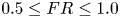


Supplementary movies
Supplementary movies are available at https://doi.org/10.1017/jfm.2023.549.
Acknowledgements
We would like to acknowledge the staff of the departmental workshop for their fabrication and machining work. Assistance in post-processing and fruitful discussions with lab mates especially with Mr G. Balamurugan is also gratefully acknowledged.
Declaration of interests
The authors report no conflict of interest.


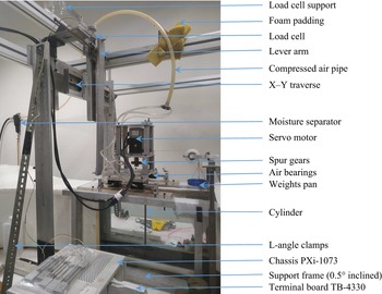
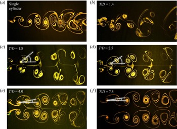


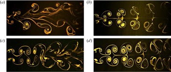


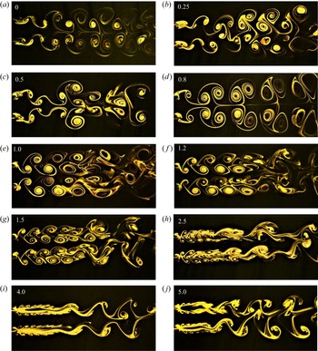


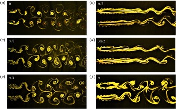


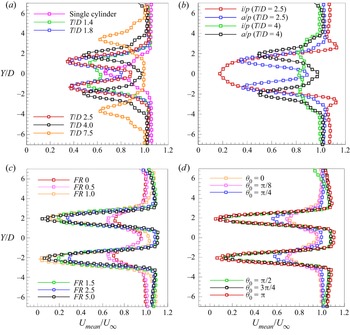


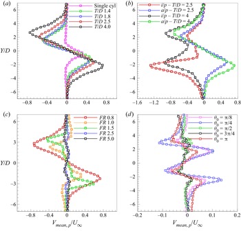


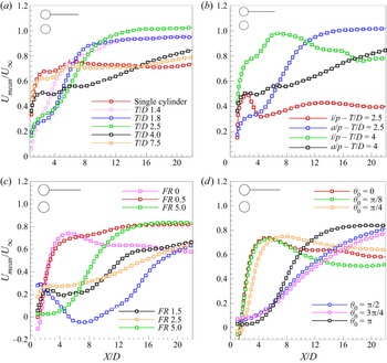


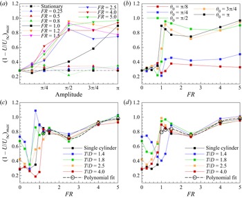


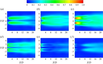


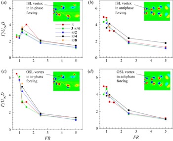


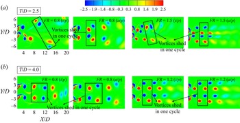


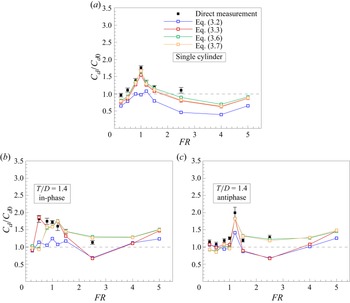


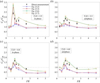


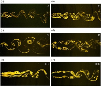
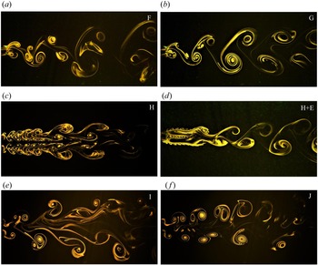


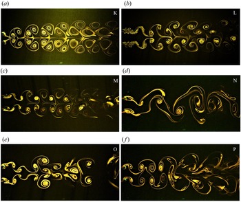


 Open access