


1. Introduction
Viscoelastic fluid flows in non-uniform geometries consisting of contractions or expansions occur in physiological flows, e.g. arterial flows that may have such shape changes due to thrombus formation (Westein et al. Reference Westein, van der Meer, Kuijpers, Frimat, van den Berg and Heemskerk2013), and in various industrial applications (Pearson Reference Pearson1985). For such flows, one of the key interests is to understand the dependence of the pressure drop  $\Delta p$ on the flow rate $q$. It is well known that adding even small amounts of polymer molecules in a Newtonian solvent may drastically change the hydrodynamic features of the flow of the solution due to polymer stretching, which generates elastic stresses in addition to viscous stresses (Bird, Armstrong & Hassager Reference Bird, Armstrong and Hassager1987; Alves, Oliveira & Pinho Reference Alves, Oliveira and Pinho2021; Steinberg Reference Steinberg2021; Datta et al. Reference Datta2022).
Pressure-driven flows of viscoelastic fluids and the corresponding flow rate–pressure drop relation have been studied extensively in various geometries, mainly through numerical simulations (Szabo, Rallison & Hinch Reference Szabo, Rallison and Hinch1997; Alves, Oliveira & Pinho Reference Alves, Oliveira and Pinho2003; Binding, Phillips & Phillips Reference Binding, Phillips and Phillips2006; Alves & Poole Reference Alves and Poole2007; Zografos et al. Reference Zografos, Hartt, Hamersky, Oliveira, Alves and Poole2020; Varchanis et al. Reference Varchanis, Tsamopoulos, Shen and Haward2022) and experimental measurements (Rothstein & McKinley Reference Rothstein and McKinley1999, Reference Rothstein and McKinley2001; Sousa et al. Reference Sousa, Coelho, Oliveira and Alves2009; Ober et al. Reference Ober, Haward, Pipe, Soulages and McKinley2013; James & Roos Reference James and Roos2021). We refer the reader to overviews given recently by Boyko & Stone (Reference Boyko and Stone2022) and Hinch, Boyko & Stone (Reference Hinch, Boyko and Stone2024).
In particular, the abrupt contraction and contraction–expansion channels have received much attention (Rothstein & McKinley Reference Rothstein and McKinley1999; Alves et al. Reference Alves, Oliveira and Pinho2003; Binding et al. Reference Binding, Phillips and Phillips2006; Ferrás et al. Reference Ferrás, Afonso, Alves, Nóbrega and Pinho2020), and  $4\,{:}\,1$ two-dimensional (2-D) and axisymmetric contraction flows have become benchmark flow problems in computational non-Newtonian fluid mechanics (Alves et al. Reference Alves, Oliveira and Pinho2021). Numerical simulations of viscoelastic fluid flow in these and other non-uniform geometries include a long downstream (exit) section to allow the stresses to reach their fully relaxed values (see, e.g. Debbaut, Marchal & Crochet Reference Debbaut, Marchal and Crochet1988; Alves et al. Reference Alves, Oliveira and Pinho2003). This is because, once perturbed from their fully relaxed values, the elastic stresses require a long distance for spatial relaxation to enable stable and converged numerical solutions. For higher Deborah ( $De$) or Weissenberg ( $Wi$) numbers (see definitions in § 2.1), a longer downstream section is required (Keiller Reference Keiller1993).
Therefore, understanding the spatial relaxation of elastic stresses, velocity and pressure is of both fundamental and practical importance, as that determines the size of the computational domain (Alves et al. Reference Alves, Oliveira and Pinho2003). However, despite extensive study of viscoelastic channel flows, the spatial relaxation of stresses and pressure in these geometries is not well understood. As a result, the length of the exit channel is currently set somewhat arbitrarily, thus motivating the development of theory. Furthermore, in many applications, it is necessary to determine the total pressure drop over the configuration for a given flow rate, thus requiring us to account for the pressure drop in the entry and exit channels. However, most studies to date focused on the non-uniform region or close vicinity of the abrupt contraction and reported a suitably non-dimensionalized so-called Couette correction (or excess pressure drop), rather than the total non-dimensional pressure drop in the entire configuration (see, e.g. Rothstein & McKinley Reference Rothstein and McKinley1999; Alves et al. Reference Alves, Oliveira and Pinho2003; Binding et al. Reference Binding, Phillips and Phillips2006), presumably due to the arbitrariness of the exit channel length in simulations.
One widely used approach to obtaining theoretical results in different viscoelastic fluid flow problems relies on considering the weakly viscoelastic limit by applying a perturbation expansion in powers of the Deborah or Weissenberg number, which are assumed to be small (see, e.g. Datt et al. Reference Datt, Natale, Hatzikiriakos and Elfring2017; Datt, Nasouri & Elfring Reference Datt, Nasouri and Elfring2018; Datt & Elfring Reference Datt and Elfring2019; Gkormpatsis et al. Reference Gkormpatsis, Gryparis, Housiadas and Beris2020; Dandekar & Ardekani Reference Dandekar and Ardekani2021; Housiadas, Binagia & Shaqfeh Reference Housiadas, Binagia and Shaqfeh2021; Su et al. Reference Su, Castillo, Pak, Zhu and Zenit2022). In particular, there have been many applications of such an expansion in conjunction with lubrication theory in studying thin films and tribology problems (Ro & Homsy Reference Ro and Homsy1995; Tichy Reference Tichy1996; Sawyer & Tichy Reference Sawyer and Tichy1998; Zhang, Matar & Craster Reference Zhang, Matar and Craster2002; Saprykin, Koopmans & Kalliadasis Reference Saprykin, Koopmans and Kalliadasis2007; Ahmed & Biancofiore Reference Ahmed and Biancofiore2021; Gamaniel, Dini & Biancofiore Reference Gamaniel, Dini and Biancofiore2021; Ahmed & Biancofiore Reference Ahmed and Biancofiore2023). Recently, we have applied lubrication theory and such an expansion in powers of  $De$, developing a reduced-order model for the steady flow of an Oldroyd-B fluid in a slowly varying, arbitrarily shaped 2-D channel (Boyko & Stone Reference Boyko and Stone2022). We provided analytical expressions for the velocity and stress fields and the flow rate–pressure drop relation in the non-uniform region up to $O(De^2)$. We further exploited the reciprocal theorem (Boyko & Stone Reference Boyko and Stone2021, Reference Boyko and Stone2022) to obtain the flow rate–pressure drop relation at the next order, $O(De^3)$. Housiadas & Beris (Reference Housiadas and Beris2023) extended the low-Deborah-number lubrication analysis of Boyko & Stone (Reference Boyko and Stone2022) to much higher asymptotic orders and provided analytical expressions for the pressure drop up to $O(De^8$).
However, the low-Deborah-number analysis cannot accurately capture the behaviour at high  $De$ numbers where there are significant elastic stresses. Another approach to simplifying the governing equations while capturing the underlying physics at non-small Deborah numbers is to consider the ultra-dilute limit (Remmelgas, Singh & Leal Reference Remmelgas, Singh and Leal1999; Moore & Shelley Reference Moore and Shelley2012; Li, Thomases & Guy Reference Li, Thomases and Guy2019; Mokhtari et al. Reference Mokhtari, Latché, Quintard and Davit2022), $\tilde {\beta }=\mu _{p}/\mu _{0} \ll 1$, where $\mu _{p}$ is the polymer contribution to the total zero-shear-rate viscosity $\mu _{0}$ of the polymer solution. Physically, the ultra-dilute limit corresponds to a low concentration of polymer molecules in a Newtonian solvent, such that the viscosity of the polymer solution, $\mu _{0}$, is only slightly larger than the solvent viscosity, $\mu _{s}$ (Remmelgas et al. Reference Remmelgas, Singh and Leal1999; Mokhtari et al. Reference Mokhtari, Latché, Quintard and Davit2022). Furthermore, the limit $\tilde {\beta }=\mu _{p}/\mu _{0} \ll 1$ is closely related to the diluteness criterion of a constant shear-viscosity viscoelastic Boger fluid (Moore & Shelley Reference Moore and Shelley2012). In the ultra-dilute limit, the flow field approximated as Newtonian creates elastic stresses that are not coupled back to change the flow. These elastic stresses can then be used to find the correction to the velocity and pressure fields due to fluid viscoelasticity, even at high Deborah numbers. Previous studies used this approach to determine the structure of the stress distribution in the flow around a cylinder (Renardy Reference Renardy2000), a sphere (Moore & Shelley Reference Moore and Shelley2012) and arrays of cylinders (Mokhtari et al. Reference Mokhtari, Latché, Quintard and Davit2022), as well as in stagnation (Becherer, Van Saarloos & Morozov Reference Becherer, Van Saarloos and Morozov2009; Van Gorder, Vajravelu & Akyildiz Reference Van Gorder, Vajravelu and Akyildiz2009) and cross-slot (Remmelgas et al. Reference Remmelgas, Singh and Leal1999) flows.
In this work, we continue our theoretical studies (Boyko & Stone Reference Boyko and Stone2022; Hinch et al. Reference Hinch, Boyko and Stone2024) of the pressure-driven flow of the Oldroyd-B fluid in slowly varying, arbitrarily shaped, narrow channels. In contrast to Boyko & Stone (Reference Boyko and Stone2022), who focused only on the flow through a non-uniform channel in the low-Deborah-number limit, and Hinch et al. (Reference Hinch, Boyko and Stone2024), who studied numerically the flow through a contraction, expansion and constriction for order-one Deborah numbers, and also provided an asymptotic description at high Deborah numbers, the current work examines the ultra-dilute limit and arbitrary values of the Deborah number. Specifically, we analyse the flow of the Oldroyd-B fluid in a contracting geometry and the relaxation of the elastic stresses and pressure in the exit channel. We apply the lubrication approximation and use a one-way coupling between the velocity and polymer stresses to derive semi-analytical expressions for the conformation tensor in the contraction and the exit channel for arbitrary values of the Deborah number in the ultra-dilute limit. These semi-analytical expressions allow us to calculate the pressure drop and elucidate the relaxation of the elastic stresses and pressure in the exit channel for all  $De$. We provide analytical expressions for the conformation tensor and the pressure drop in the high-Deborah-number limit, which are consistent with recent results of Hinch et al. (Reference Hinch, Boyko and Stone2024), thus complementing our previous low-Deborah-number lubrication analysis (Boyko & Stone Reference Boyko and Stone2022). Furthermore, we analyse the viscoelastic boundary layer near the walls at high Deborah numbers and derive the boundary-layer asymptotic solutions. Given the well-known lack of accuracy and convergence difficulties associated with the high-Weissenberg-number problem in numerical simulations (Owens & Phillips Reference Owens and Phillips2002; Alves et al. Reference Alves, Oliveira and Pinho2021), our analytical and semi-analytical results for the ultra-dilute limit, valid at high Deborah numbers, are of fundamental importance as they may serve to validate simulation predictions or be compared with experimental measurements to understand more about the applicability of model constitutive equations.
2. Problem formulation and governing equations
We analyse the incompressible steady flow of a viscoelastic fluid in a slowly varying and symmetric 2-D contraction of height  $2h(z)$ and length $\ell$, where $h(z)\ll \ell$, as illustrated in figure 1. Upstream of the contraction inlet ( $z=0$) there is an entry channel of height $2h_{0}$ and length $\ell _{0}$, and downstream of the contraction outlet ( $z=\ell$) there is an exit channel of height $2h_{\ell }$ and length $\ell _{\ell }$. The fluid flow has velocity $\boldsymbol {u}$ and pressure distribution $p$, which are induced by an imposed flow rate $q$ (per unit depth). Our primary interest is to determine the pressure drop $\Delta p$ over the contraction region and the spatial relaxation of pressure and elastic stresses in the exit channel. For our analysis, we shall employ two different systems of coordinates. The first is Cartesian coordinates $(z,y)$ and $(z_{\ell },y)$, where the $z$ and $z_{\ell }=z-\ell$ axes lie along the symmetry midplane of the channel (dashed-dotted line) and $y$ is in the direction of the shortest dimension. The second one is orthogonal curvilinear coordinates $(\xi,\eta )$ defined in § 2.3.

Figure 1. Schematic illustration of the 2-D configuration consisting of a slowly varying and symmetric contraction of height  $2h(z)$ and length $\ell$ ( $h\ll \ell$). The contraction is connected to two long straight channels of height $2h_{0}$ and $2h_{\ell }$, respectively, up- and downstream and contains a viscoelastic fluid steadily driven by the imposed flow rate $q$.
$q$.
We consider low-Reynolds-number flows so that the fluid motion is governed by the continuity equation and Cauchy momentum equations in the absence of inertia
 \begin{equation} \boldsymbol{\nabla}\boldsymbol{\cdot} \boldsymbol{u}=0,\quad\boldsymbol{\nabla}\boldsymbol{\cdot} \boldsymbol{\sigma}=\boldsymbol{0}.\end{equation}
To describe the viscoelastic behaviour of the fluid, we use the Oldroyd-B constitutive model (Oldroyd Reference Oldroyd1950), which represents the most simple combination of viscous and elastic stresses and is used widely to describe the flow of viscoelastic Boger fluids, characterized by a constant shear viscosity. The Oldroyd-B equation can be derived from microscopic principles by modelling polymer molecules as elastic dumbbells, which follow a linear Hooke's law for the restoring force as they are advected and stretched by the flow. The corresponding stress tensor  $\boldsymbol {\sigma }$ is
 \begin{equation} \boldsymbol{\sigma}={-}p\boldsymbol{\mathsf{I}}+2\mu_{s}\boldsymbol{\mathsf{E}}+\boldsymbol{\tau}_{\!p},\end{equation}
where the first term on the right-hand side of (2.2) is the pressure contribution, the second term is the viscous stress contribution of a Newtonian solvent with a constant viscosity  $\mu _{s}$, where $\boldsymbol{\mathsf{E}}=(\boldsymbol {\nabla }\boldsymbol {u}+(\boldsymbol {\nabla }\boldsymbol {u})^{\mathrm {T}})/2$ is the rate-of-strain tensor, and the last term, $\boldsymbol {\tau }_{p}$, is the polymer contribution. We note that $\boldsymbol{\mathsf{I}}$ in (2.2) is the identity tensor and T is the transpose operator on a tensor.
For the Oldroyd-B model, the polymer contribution to the stress tensor  $\boldsymbol {\tau }_{p}$ can be expressed in terms of the (symmetric) conformation tensor (or the deformation of the microstructure) $\boldsymbol{\mathsf{A}}$ as (Bird et al. Reference Bird, Armstrong and Hassager1987; Larson Reference Larson1988; Morozov & Spagnolie Reference Morozov and Spagnolie2015)
 \begin{equation} \boldsymbol{\tau}_{\!p}=G(\boldsymbol{\mathsf{A}}-\boldsymbol{\mathsf{I}})=\frac{\mu_{p}}{\lambda}(\boldsymbol{\mathsf{A}}-\boldsymbol{\mathsf{I}}),\end{equation}
where  $G$ is the elastic modulus, $\lambda$ is the relaxation time and $\mu _{p}=G \lambda$ is the polymer contribution to the shear viscosity at zero shear rate. It is also convenient to introduce the total zero-shear-rate viscosity $\mu _0=\mu _s+\mu _p$.
The evolution equation for the deformation of the microstructure  $\boldsymbol{\mathsf{A}}$ of the Oldroyd-B model fluid is given at steady state as (Bird et al. Reference Bird, Armstrong and Hassager1987; Larson Reference Larson1988; Morozov & Spagnolie Reference Morozov and Spagnolie2015)
 \begin{equation} \boldsymbol{u}\boldsymbol{\cdot}\boldsymbol{\nabla}\boldsymbol{\mathsf{A}}-(\boldsymbol{\nabla}\boldsymbol{u})^{\mathrm{T}} \boldsymbol{\cdot}\boldsymbol{\mathsf{A}}-\boldsymbol{\mathsf{A}}\boldsymbol{\cdot}(\boldsymbol{\nabla}\boldsymbol{u})={-}\frac{1}{\lambda}(\boldsymbol{\mathsf{A}}-\boldsymbol{\mathsf{I}}).\end{equation}
2.1. Scaling analysis and non-dimensionalization
We consider narrow configurations, in which  $h(z)\ll \ell$, $h_{0}$ is the half-height at $z=0$, and $u_{c}=q/2h_{0}$ is the characteristic velocity scale set by the cross-sectionally averaged velocity. We introduce non-dimensional variables based on lubrication theory (Tichy Reference Tichy1996; Zhang et al. Reference Zhang, Matar and Craster2002; Saprykin et al. Reference Saprykin, Koopmans and Kalliadasis2007; Ahmed & Biancofiore Reference Ahmed and Biancofiore2021; Boyko & Stone Reference Boyko and Stone2022)
 \begin{gather} Z=\frac{z}{\ell},\quad Y=\frac{y}{h_{0}}, \quad U_{z}=\frac{u_{z}}{u_{c}},\quad U_{y}=\frac{u_{y}}{\epsilon u_{c}}, \end{gather}
 \begin{gather}P=\frac{p}{\mu_{0}u_{c}\ell/h_{0}^{2}},\quad\Delta P=\frac{\Delta p}{\mu_{0}u_{c}\ell/h_{0}^{2}},\quad H=\frac{h}{h_{0}}, \end{gather}
 \begin{gather}\tilde{A}_{zz}=\epsilon^{2}A_{zz},\quad\tilde{A}_{zy}=\epsilon A_{zy},\quad\tilde{A}_{yy}=A_{yy}, \end{gather}
where we have introduced the aspect ratio of the configuration, which is assumed to be small
 \begin{equation} \epsilon=\frac{h_{0}}{\ell}\ll1,\end{equation}
the contraction ratio
 \begin{equation} H_{\ell}=\frac{h_{\ell}}{h_{0}},\end{equation}
the viscosity ratios
 \begin{equation} \tilde{\beta}=\frac{\mu_{p}}{\mu_{s}+\mu_{p}}=\frac{\mu_{p}}{\mu_{0}}\quad\mbox{and}\quad\beta=1-\tilde{\beta}=\frac{\mu_{s}}{\mu_{0}},\end{equation}
and the Deborah and Weissenberg numbers
 \begin{equation} De=\frac{\lambda u_{c}}{\ell}\quad\mbox{and}\quad Wi=\frac{\lambda u_{c}}{h_{0}}.\end{equation}
For lubrication flows through the narrow geometries that we consider, there is a difference between the Deborah and Weissenberg numbers because of the two distinct length scales. The Weissenberg number  $Wi$ is the product of the relaxation time scale of the fluid, $\lambda$, and the characteristic shear rate of the flow, $u_{c}/h_{0}$. On the other hand, the Deborah number $De$ is the ratio of the relaxation time, $\lambda$, to the residence time in the contraction region, $\ell /u_{c}$, or alternatively, the product of the relaxation time and the characteristic extensional rate of the flow (Tichy Reference Tichy1996; Zhang et al. Reference Zhang, Matar and Craster2002; Saprykin et al. Reference Saprykin, Koopmans and Kalliadasis2007; Ahmed & Biancofiore Reference Ahmed and Biancofiore2021). The Deborah and Weissenberg numbers are related through $De=\epsilon Wi$, and for narrow geometries with $\epsilon \ll 1$, $De$ can be small while keeping $Wi =O(1)$.
Similar to our previous study (Boyko & Stone Reference Boyko and Stone2022), we non-dimensionalize the pressure using the total zero-shear-rate viscosity  $\mu _{0}=\mu _{s}+\mu _{p}$. However, for convenience, we non-dimensionalize the height based on the entry height rather than the exit height. In addition, unlike our previous study, we do not scale the deformation of the microstructure with $De^{-1}$. Our current scaling is consistent with a fully developed unidirectional flow of an Oldroyd-B fluid in a straight channel, which yields $\tilde {A}_{zz}=O(De^2)$, $\tilde {A}_{zy}=O(De)$ and $\tilde {A}_{yy}=O(1)$; see (2.10d)–(2.10f) and (2.16). This scaling is convenient when considering arbitrary and large values of the Deborah number.
Note that, in both Hinch et al. (Reference Hinch, Boyko and Stone2024) and here, the channel height is  $2h$, but the total flow rate per unit depth in the former is $2q$, whereas in this work it is $q$ as in Boyko & Stone (Reference Boyko and Stone2022). All results are compatible because the variables used for the non-dimensionalization are the same, i.e. the expressions for the characteristic velocity, characteristic pressure and the Deborah number are the same.
2.2. Dimensionless lubrication equations in Cartesian coordinates
Using the non-dimensionalization (2.5)–(2.9a,b), to the leading order in  $\epsilon$, the governing equations (2.1)–(2.4) take the form
 \begin{gather} \frac{\partial U_{z}}{\partial Z}+\frac{\partial U_{y}}{\partial Y}=0, \end{gather}
 \begin{gather}\frac{\partial P}{\partial Z}=(1-\tilde{\beta})\frac{\partial^{2}U_{z}}{\partial Y^{2}}+\frac{\tilde{\beta}}{De}\left(\frac{\partial\tilde{A}_{zz}}{\partial Z}+\frac{\partial\tilde{A}_{zy}}{\partial Y}\right), \end{gather}
 \begin{gather}\frac{\partial P}{\partial Y}=0, \end{gather}
 \begin{gather}U_{z}\frac{\partial \tilde{A}_{zz}}{\partial Z}+U_{y}\frac{\partial \tilde{A}_{zz}}{\partial Y}-2\frac{\partial U_{z}}{\partial Z}\tilde{A}_{zz}-2\frac{\partial U_{z}}{\partial Y}\tilde{A}_{zy}={-}\frac{1}{De}\tilde{A}_{zz}, \end{gather}
 \begin{gather}U_{z}\frac{\partial \tilde{A}_{zy}}{\partial Z}+U_{y}\frac{\partial \tilde{A}_{zy}}{\partial Y}-\frac{\partial U_{y}}{\partial Z}\tilde{A}_{zz}-\frac{\partial U_{z}}{\partial Y}\tilde{A}_{yy}={-}\frac{1}{De}\tilde{A}_{zy}, \end{gather}
 \begin{gather}U_{z}\frac{\partial \tilde{A}_{yy}}{\partial Z}+U_{y}\frac{\partial \tilde{A}_{yy}}{\partial Y}-2\frac{\partial U_{y}}{\partial Z}\tilde{A}_{zy}-2\frac{\partial U_{y}}{\partial Y}\tilde{A}_{yy}={-}\frac{1}{De}(\tilde{A}_{yy}-1). \end{gather}
From (2.10c), it follows that  $P=P(Z)$, i.e. the pressure is independent of $Y$ up to $O(\epsilon ^2)$, consistent with the classical lubrication approximation. We note that the scaled $\tilde {A}_{zz}$ on the right-hand side of (2.10d) relaxes to $\epsilon ^2$, which is neglected at the leading order in $\epsilon$.
2.3. Orthogonal curvilinear coordinates for a slowly varying geometry
For our theoretical analysis, it is convenient to transform the geometry of the contraction from the Cartesian coordinates ( $Z,Y$) to curvilinear coordinates ( $\xi,\eta$), as illustrated in figure 2, with the mapping (Hinch et al. Reference Hinch, Boyko and Stone2024)
 \begin{equation} \xi=Z-\frac{1}{2}\epsilon^{2}\frac{H'(Z)}{H(Z)}(H(Z)^{2}-Y^{2})+O(\epsilon^{4}), \quad\eta=\frac{Y}{H(Z)}.\end{equation}
As shown in Appendix A, the curvilinear coordinates ( $\xi,\eta$) are orthogonal with a relative error of $O(\epsilon ^{4})$, i.e. $\boldsymbol {\nabla }\xi \boldsymbol {\cdot }\boldsymbol {\nabla }\eta =O(\epsilon ^{4})$.

Figure 2. Schematic illustration of the orthogonal curvilinear coordinates ( $\xi,\eta$) for a slowly varying geometry. The coordinate $\xi$ is constant along vertical grid lines, and $\eta$, defined in (2.11a,b), is constant along the curves going from left to right.
Hereafter, we use  $\boldsymbol {u}=u\boldsymbol {e}_{\xi }+\upsilon \boldsymbol {e}_{\eta }$ and $\boldsymbol{\mathsf{A}}=A_{11}\boldsymbol {e}_{\xi }\boldsymbol {e}_{\xi }+A_{12}(\boldsymbol {e}_{\xi } \boldsymbol {e}_{\eta }+\boldsymbol {e}_{\eta }\boldsymbol {e}_{\xi })+A_{22} \boldsymbol {e}_{\eta }\boldsymbol {e}_{\eta }$ to denote, respectively, the components of velocity and deformation of the microstructure in curvilinear coordinates ( $\xi,\eta$). The corresponding non-dimensional velocity components in different coordinates are related through (see Appendix A)
 \begin{equation} U_{z}=U-\epsilon^{2}\eta H'(\xi) V, \quad U_{y}=\eta H'(\xi) U+V.\end{equation}
Similarly, the scaled conformation tensor components in different coordinates are related through (see Appendix A)
 \begin{gather} \tilde{A}_{zz}=\tilde{A}_{11}+O(\epsilon^{2}), \end{gather}
 \begin{gather}\tilde{A}_{zy}=\tilde{A}_{12}+\eta H'(\xi)\tilde{A}_{11}+O(\epsilon^{2}), \end{gather}
 \begin{gather}\tilde{A}_{yy}=\tilde{A}_{22}+2\eta H'(\xi)\tilde{A}_{12}+\eta^2 (H'(\xi))^2\tilde{A}_{11}+O(\epsilon^{2}). \end{gather}
Finally, we note that, since there is only a  $O(\epsilon ^{2})$ difference between the $\xi$- and $z$-directions, for convenience, we continue to use $Z$ rather than $\xi$ in curvilinear coordinates.
2.4. Dimensionless lubrication equations in orthogonal curvilinear coordinates
Using the mapping (2.11a,b), the governing equations (2.10) take the form in curvilinear coordinates (Hinch et al. Reference Hinch, Boyko and Stone2024)
 \begin{gather} \frac{\partial(HU)}{\partial Z}+\frac{\partial V}{\partial\eta}=0, \end{gather}
 \begin{gather}\frac{\mathrm{d}P}{\mathrm{d}Z}=(1-\tilde{\beta})\frac{1}{H^{2}}\frac{\partial^{2}U}{\partial\eta^{2}}+\frac{\tilde{\beta}}{De}\left(\frac{1}{H}\frac{\partial(H\tilde{A}_{11})}{\partial Z}+\frac{1}{H}\frac{\partial\tilde{A}_{12}}{\partial\eta}\right), \end{gather}
 \begin{gather}U\frac{\partial\tilde{A}_{11}}{\partial Z}+\frac{V}{H}\frac{\partial\tilde{A}_{11}}{\partial\eta}-2\frac{\partial U}{\partial Z}\tilde{A}_{11}-\frac{2}{H}\frac{\partial U}{\partial\eta}\tilde{A}_{12}={-}\frac{1}{De}\tilde{A}_{11}, \end{gather}
 \begin{gather}U\frac{\partial\tilde{A}_{12}}{\partial Z}+\frac{V}{H}\frac{\partial\tilde{A}_{12}}{\partial\eta}-H\frac{\partial}{\partial Z}\left(\frac{V}{H}\right)\tilde{A}_{11}-\frac{1}{H}\frac{\partial U}{\partial\eta}\tilde{A}_{22}={-}\frac{1}{De}\tilde{A}_{12}, \end{gather}
 \begin{gather}U\frac{\partial\tilde{A}_{22}}{\partial Z}+\frac{V}{H}\frac{\partial\tilde{A}_{22}}{\partial\eta}-2H\frac{\partial}{\partial Z}\left(\frac{V}{H}\right)\tilde{A}_{12}+2\frac{\partial U}{\partial Z}\tilde{A}_{22}={-}\frac{1}{De}(\tilde{A}_{22}-1). \end{gather}
The corresponding boundary conditions on the velocity are
 \begin{equation} U(Z,1)=0,\quad V(Z,1)=0,\quad \frac{\partial U} {\partial\eta}(Z,0)=0,\quad H(Z)\int_{0}^{1}U(Z,\eta)\,\mathrm{d}\eta=1,\end{equation}
which represent, respectively, the no-slip and no-penetration boundary conditions along the channel walls, the symmetry boundary condition at the centreline and the integral mass conservation along the channel. In addition, we assume a fully developed unidirectional Poiseuille flow in the straight entry channel and the corresponding deformation of the microstructure
 \begin{equation} \tilde{A}_{11}=\frac{18De^{2}}{H^{4}}\eta^{2},\quad \tilde{A}_{12}={-}\frac{3De}{H^{2}}\eta,\quad \tilde{A}_{22}=1,\end{equation}
with  $H \equiv 1$ at the entrance. We also assume that, far downstream in the exit channel, the deformation of the microstructure attains a fully relaxed value, given by (2.16) with $H \equiv H_{\ell }$.
2.5. Pressure drop across the non-uniform region in the lubrication limit
In this subsection, we show that one can calculate the pressure drop without solving directly for the velocity field. To this end, we first integrate by parts the integral constraint (2.15d), repeatedly, using (2.15a) and (2.15c), e.g. (Hinch et al. Reference Hinch, Boyko and Stone2024)
 \begin{align}
\frac{1}{H(Z)}&=\int_{0}^{1}U\,\mathrm{d}\eta=\underset{0}{\underbrace{\left.\eta
U\right|_{0}^{1}}}-\int_{0}^{1}\eta\frac{\partial
U}{\partial\eta}\mathrm{d}\eta=\underset{0}{\underbrace{\left.\frac{1}{2}(1-\eta^{2})\frac{\partial
U}{\partial\eta}\right|_{0}^{1}}}-\frac{1}{2}\int_{0}^{1}(1-\eta^{2})\frac{\partial^{2}U}{\partial\eta^{2}}\mathrm{d}\eta.\end{align}
\begin{align}
\frac{1}{H(Z)}&=\int_{0}^{1}U\,\mathrm{d}\eta=\underset{0}{\underbrace{\left.\eta
U\right|_{0}^{1}}}-\int_{0}^{1}\eta\frac{\partial
U}{\partial\eta}\mathrm{d}\eta=\underset{0}{\underbrace{\left.\frac{1}{2}(1-\eta^{2})\frac{\partial
U}{\partial\eta}\right|_{0}^{1}}}-\frac{1}{2}\int_{0}^{1}(1-\eta^{2})\frac{\partial^{2}U}{\partial\eta^{2}}\mathrm{d}\eta.\end{align}
Substituting the expression for  $\partial ^{2}U/\partial \eta ^{2}$ from (2.14b) into (2.17), we obtain
 \begin{equation} -\frac{1-\tilde{\beta}}{H(Z)^3}=\frac{1}{2}\int_{0}^{1}(1-\eta^{2})\left[\frac{\mathrm{d}P}{\mathrm{d}Z}-\frac{\tilde{\beta}}{De}\left(\frac{1}{H}\frac{\partial(H\tilde{A}_{11})}{\partial Z}+\frac{1}{H}\frac{\partial\tilde{A}_{12}}{\partial\eta}\right)\right]\mathrm{d}\eta,\end{equation}
which can be rearranged to yield the pressure gradient
 \begin{equation} \frac{\mathrm{d}P}{\mathrm{d}Z}={-}\frac{3(1-\tilde{\beta})}{H(Z)^{3}}+\frac{3 \tilde{\beta}}{2De}\int_{0}^{1}(1-\eta^{2})\left[\frac{1}{H(Z)}\frac{\partial(H(Z)\tilde{A}_{11})}{\partial Z}+\frac{1}{H(Z)}\frac{\partial\tilde{A}_{12}}{\partial\eta}\right]\mathrm{d}\eta.\end{equation}
Integrating (2.19) with respect to  $Z$ from 0 to 1 provides the pressure drop $\Delta P=P(0)-P(1)$ across the non-uniform region
 \begin{align} \Delta P&=3(1-\tilde{\beta})\int_{0}^{1}\frac{\mathrm{d}Z}{H(Z)^{3}} \nonumber\\ &\quad -\frac{3\tilde{\beta}}{2De}\int_{0}^{1}\int_{0}^{1}(1-\eta^{2})\left[\frac{1}{H(Z)} \frac{\partial(H(Z)\tilde{A}_{11})}{\partial Z}+\frac{1}{H(Z)}\frac{\partial\tilde{A}_{12}}{\partial\eta}\right]\mathrm{d}\eta\,\mathrm{d}Z. \end{align}
Using integration by parts, (2.20) can be expressed as
 \begin{align} \Delta P&= 3(1-\tilde{\beta})\int_{0}^{1}\frac{\mathrm{d}Z}{H(Z)^{3}}+\frac{3 \tilde{\beta}}{2De}\int_{0}^{1}(1-\eta^{2})\left[\tilde{A}_{11}(0,\eta)-\tilde{A}_{11}(1,\eta)\right] \mathrm{d}\eta \nonumber\\ &\quad -\frac{3\tilde{\beta}}{2De}\int_{0}^{1}\left[\frac{H'(Z)}{H(Z)}\left(\int_{0}^{1}(1-\eta^{2})\tilde{A}_{11}\, \mathrm{d}\eta\right)\right]\mathrm{d}Z \nonumber\\ &\quad -\frac{3\tilde{\beta}}{De}\int_{0}^{1}\left[\frac{1}{H(Z)}\int_{0}^{1}\eta\tilde{A}_{12}\,\mathrm{d}\eta \right]\mathrm{d}Z, \end{align}
where prime indicates a derivative with respect to  $Z$.
$Z$.
Equation (2.21) resembles the result of an application of the reciprocal theorem previously derived for the pressure drop of the flow of an Oldroyd-B fluid in a slowly varying channel (Boyko & Stone Reference Boyko and Stone2021, Reference Boyko and Stone2022). The first term on the right-hand side of (2.21) represents the viscous contribution of the Newtonian solvent to the pressure drop. The second term represents the contribution of the elastic normal stress difference at the inlet and outlet of the non-uniform channel. The third term represents the contribution of the elastic normal stresses that arise due to the spatial variations in the channel shape, which is a contribution that is absent in a straight channel. Finally, the last term represents the elastic contribution due to shear stresses within the fluid domain of the non-uniform channel. It should be noted that we do not assume a priori the particular shape of the channel  $H(Z)$ but rather consider a flow in a slowly varying channel of arbitrary shape $H(Z)$.
3. Low- $\tilde {\beta }$ lubrication analysis in a slowly varying region

In the previous section, we obtained the dimensionless equations (2.14), which are governed by the two non-dimensional parameters,  $\tilde {\beta }$ and $De$, in the lubrication limit ( $\epsilon \ll 1$). In this section, we derive analytical expressions for the velocity, conformation tensor and the $q-\Delta p$ relation for the pressure-driven flow of a very dilute viscoelastic Oldroyd-B fluid, $\tilde {\beta }=\mu _{p}/\mu _{0}\ll 1$ in a slowly varying channel of arbitrary shape $H(Z)$.
In contrast to our previous study that employed a low-Deborah-number lubrication analysis (Boyko & Stone Reference Boyko and Stone2022), in this work, we assume  $De=O(1)$ and consider the ultra-dilute limit, $\tilde {\beta }\ll 1$ (see Remmelgas et al. Reference Remmelgas, Singh and Leal1999; Moore & Shelley Reference Moore and Shelley2012; Li et al. Reference Li, Thomases and Guy2019; Mokhtari et al. Reference Mokhtari, Latché, Quintard and Davit2022). To this end, we seek solutions of the form
 \begin{equation} \left(\begin{array}{c} U\\ V\\ P\\ \tilde{A}_{11}\\ \tilde{A}_{12}\\ \tilde{A}_{22} \end{array}\right)=\left(\begin{array}{c} U_{0}\\ V_{0}\\ P_{0}\\ \tilde{A}_{11,0}\\ \tilde{A}_{12,0}\\ \tilde{A}_{22,0} \end{array}\right)+\tilde{\beta}\left(\begin{array}{c} U_{1}\\ V_{1}\\ P_{1}\\ \tilde{A}_{11,1}\\ \tilde{A}_{12,1}\\ \tilde{A}_{22,1} \end{array}\right)+O(\epsilon^{2},\tilde{\beta}^{2}).\end{equation}
The ultra-dilute limit represents a one-way coupling between the velocity and pressure fields and the deformation of the microstructure (polymer stresses or conformation tensor). At leading order, the velocity and pressure are Newtonian, and the deformation of the microstructure (i.e. polymer stresses) arises from this Newtonian flow. Accordingly, the velocity and pressure at  $O(\tilde {\beta })$ arise due to leading-order polymer stresses. In the next subsections, we provide closed-form asymptotic expressions for the velocity field and conformation tensor components at $O(\tilde {\beta }^{0})$ and the pressure drop up to $O(\tilde {\beta })$.
We note that the viscosity ratio  $\tilde {\beta }=\mu _{p}/\mu _{0}$ is related to the so-called concentration of the polymers $c=\mu _{p}/\mu _{s}$ through $\tilde {\beta }=c/(c+1)$. Thus, at the leading order, the limits $\tilde {\beta }\ll 1$ and $c\ll 1$ are identical.
3.1. Velocity, conformation and pressure drop at the leading order in $\tilde {\beta }$

Substituting (3.1) into (2.14a)–(2.14b) and considering the leading order in  $\tilde {\beta }$, the continuity and momentum equations take the form
 \begin{equation} \frac{\partial(HU_{0})}{\partial Z}+\frac{\partial V_{0}}{\partial\eta}=0 \quad\hbox{and}\quad \frac{\mathrm{d}P_0}{\mathrm{d}Z}=\frac{1}{H^{2}}\frac{\partial^{2}U_{0}}{\partial\eta^{2}}, \end{equation}
subject to the boundary conditions
 \begin{equation} U_{0}(Z,1)=0,\quad V_{0}(Z,1)=0,\quad \frac{\partial U_{0}}{\partial\eta}(Z,0)=0,\quad H(Z)\int_{0}^{1}U_{0}(Z,\eta)\,\mathrm{d}\eta=1.\end{equation}
The solutions for the axial velocity  $U_0$ and the pressure drop $\Delta P_{0}$ at the leading order are well known (see, e.g. Boyko & Stone Reference Boyko and Stone2022)
 \begin{equation} U_{0}=\frac{3}{2}\frac{1}{H(Z)}(1-\eta^{2})\quad\hbox{and}\quad \Delta P_{0}=3\int_{0}^{1}\frac{\mathrm{d}Z}{H(Z)^{3}}.\end{equation}
Substituting (3.4a) into the continuity equation (3.2a) and using (3.3b), yields
 \begin{equation} V_{0}\equiv0.\end{equation}
From (3.5), it follows that, in orthogonal curvilinear coordinates, the velocity in the  $\eta$-direction is identically zero at $O(\tilde {\beta }^{0})$, in contrast to the Cartesian coordinates where $U_{y,0}=(3/2)H'(Z)Y(H(Z)^{2}-Y^{2})/H(Z)^{4}$. As we shall see, this fact significantly simplifies the theoretical analysis and allows us to derive closed-form expressions for the components of the conformation tensor.
Using (3.5), at leading order in  $\tilde {\beta }$, the equations for the conformation tensor components, (2.14c)–(2.14e), simplify to
 \begin{gather} U_{0}\frac{\partial\tilde{A}_{22,0}}{\partial Z}+2\frac{\partial U_{0}}{\partial Z}\tilde{A}_{22,0}={-}\frac{1}{De}(\tilde{A}_{22,0}-1), \end{gather}
 \begin{gather}U_{0}\frac{\partial\tilde{A}_{12,0}}{\partial Z}-\frac{1}{H}\frac{\partial U_{0}}{\partial\eta}\tilde{A}_{22,0}={-}\frac{1}{De}\tilde{A}_{12,0}, \end{gather}
 \begin{gather}U_{0}\frac{\partial\tilde{A}_{11,0}}{\partial Z}-2\frac{\partial U_{0}}{\partial Z}\tilde{A}_{11,0}-\frac{2}{H}\frac{\partial U_{0}}{\partial\eta}\tilde{A}_{12,0}={-}\frac{1}{De}\tilde{A}_{11,0}, \end{gather}
subject to the boundary conditions
 \begin{equation} \tilde{A}_{11,0}(0,\eta)=18De^{2}\eta^{2},\quad\tilde{A}_{12,0}(0,\eta)={-}3De\eta, \quad\tilde{A}_{22,0}(0,\eta)=1.\end{equation}
Equations (3.6) represent a set of one-way coupled first-order semi-linear partial differential equations that can be solved first for  $\tilde {A}_{22,0}$, followed by $\tilde {A}_{12,0}$ and then for $\tilde {A}_{11,0}$.
Solving (3.6) together with (3.7), we obtain closed-form expressions for  $\tilde {A}_{22,0}$, $\tilde {A}_{12,0}$ and $\tilde {A}_{11,0}$ for arbitrary values of $De$ and the shape function $H(Z)$
 \begin{gather} \frac{\tilde{A}_{22,0}}{H(Z)^{2}}=\exp(\,{f(DeU_{0}(Z,\eta))}) \left[1+\int_{0}^{Z}\exp({-f(DeU_{0}(\tilde{Z},\eta))}) \frac{1}{DeU_{0}(\tilde{Z},\eta)H(\tilde{Z})^2}\mathrm{d}\tilde{Z}\right], \end{gather}
 \begin{gather}\frac{\tilde{A}_{12,0}}{({-}3De\eta)}=\exp(\,{f(DeU_{0}(Z,\eta))}) \left[1\!+\!\int_{0}^{Z}\exp({-f(DeU_{0}(\tilde{Z},\eta))}) \frac{\tilde{A}_{22,0}(\tilde{Z},\eta)}{DeU_{0}(\tilde{Z},\eta)H(\tilde{Z})^2}\mathrm{d}\tilde{Z}\right], \end{gather}
 \begin{align} &\frac{\tilde{A}_{11,0}}{18De^{2}\eta^{2}/H(Z)^2}\nonumber\\ &\quad =\exp(\,{f(DeU_{0}(Z,\eta))})\left[1+\int_{0}^{Z}\exp({-f(DeU_{0}(\tilde{Z},\eta))}) \frac{\tilde{A}_{12,0}(\tilde{Z},\eta)}{({-}3\eta De)DeU_{0}(\tilde{Z},\eta)}\mathrm{d}\tilde{Z}\right], \end{align}
where  $f(DeU_{0}(Z,\eta ))$ is defined as
 \begin{equation} f(DeU_{0}(Z,\eta))={-}\int_{0}^{Z}\frac{1}{De U_{0}(\tilde{Z},\eta)}\mathrm{d}\tilde{Z}={-}\int_{0}^{Z}\frac{2H(\tilde{Z})}{3De(1-\eta^{2})} \mathrm{d}\tilde{Z}.\end{equation}
It is worth noting that the right-hand sides of (3.8)–(3.10) depend on the product  $DeU_{0}(Z,\eta )$ and are not functions of $De$ and $\eta$ separately. Furthermore, (3.8)–(3.10) clearly show that, while the distribution of $\tilde {A}_{22,0}$ is set solely by the value at the beginning of the non-uniform region, the distribution of elastic shear and normal stresses, $\tilde {A}_{12,0}$ and $\tilde {A}_{11,0}$, are coupled to the transverse normal stress $\tilde {A}_{22,0}$. In fact, the elastic normal stress $\tilde {A}_{11,0}$ depends both on $\tilde {A}_{12,0}$ and $\tilde {A}_{22,0}$.
From (3.8)–(3.10), one might think that the conformation tensor components diverge at the wall ( $\eta =\pm 1$). However, using (3.6) and noting that $U_{0}=\partial U_{0}/\partial Z=0$ at $\eta =\pm 1$, it follows that, at the walls of the non-uniform channel,
 \begin{equation} \tilde{A}_{22,0}^{wall}=1,\quad\tilde{A}_{12,0}^{wall}={\mp}\frac{3De}{H(Z)^{2}},\quad\tilde{A}_{11,0}^{wall}= \frac{18De^{2}}{H(Z)^{4}}\quad\mathrm{for\ all} \ De.\end{equation}
In §§ 3.1.1 and 3.1.2, we provide explicit expressions for the conformation tensor components in the low- and high- $De$ limits. We also note that the results shown in our figure 4(a,c) and the work of Hinch et al. (Reference Hinch, Boyko and Stone2024) suggest the existence of a viscoelastic boundary layer near the walls in the high- $De$ limit, which we analyse in § 3.1.3.
3.1.1. Conformation tensor in the low-$De$ limit

For  $De\ll 1$, we solve the equations iteratively for the conformation tensor components (3.6) to obtain
 \begin{align} \tilde{A}_{22,0}&=1+\frac{3DeH'}{H^{2}}(1-\eta^{2})+\frac{9De^{2}[4H'^{2}-HH'']}{2H^{4}}(1-\eta^{2})^{2}\nonumber\\ &\quad+ \frac{27De^{3}[24H'^{3}-13HH'H''+H^{2}H''']}{4H^{6}}(1-\eta^{2})^{3}, \end{align}
 \begin{gather} \tilde{A}_{12,0}={-}\frac{3De}{H^{2}}\eta-\frac{18De^{2}H'}{H^{4}}\eta(1-\eta^{2}) - \frac{81De^{3}[4H'^{2}-HH'']}{2H^{6}}\eta(1-\eta^{2})^{2},\end{gather}
 \begin{gather} \tilde{A}_{11,0}=\frac{18De^{2}}{H^{4}}\eta^{2}+\frac{162De^{3}H'}{H^{6}}\eta^{2}(1-\eta^{2}) +\frac{486De^{4}[4H'{}^{2}-HH'']}{H^{8}}\eta^{2}(1-\eta^{2})^{2}.\end{gather}
We note that the low- $De$ results (3.13) are consistent with our previous work (Boyko & Stone Reference Boyko and Stone2022), in which we provided explicit expressions for $\tilde {A}_{zz}$, $\tilde {A}_{zy}$ and $\tilde {A}_{yy}$ up to $O(De^2)$ in Cartesian coordinates. For example, using (2.13c) and (3.13), $\tilde {A}_{yy}$ can be expressed as $\tilde {A}_{yy}=1+3DeH'(Z)(H(Z)^2-3Y^2)/H(Z)^4+O(De^2)$, in agreement with (3.9a) in Boyko & Stone (Reference Boyko and Stone2022).
3.1.2. Conformation tensor in the high-$De$ limit

We here provide the closed-form expressions for the conformation tensor components in the high- $De$ limit. We begin with the expression for $\tilde {A}_{22,0}$ and consider the core flow region.
For  $De\gg 1$, except close to the wall, (3.6a) reduces to
 \begin{equation} U_{0}\frac{\partial\tilde{A}_{22,0}}{\partial Z}+2\frac{\partial U_{0}}{\partial Z}\tilde{A}_{22,0}=0,\end{equation}
whose solution subject to (3.7c) is
 \begin{equation} \tilde{A}_{22,0}(Z,\eta)=\tilde{A}_{22,0}(0,\eta)\frac{U_{0}(0,\eta)^{2}}{U_{0}(Z,\eta)^{2}}=H(Z)^{2}.\end{equation}
Next, since  $\tilde {A}_{12,0}$ scales as $O(De)$ while $\tilde {A}_{22,0}$ is $O(1)$, within the core flow region in the high- $De$ limit we obtain that the first term in (3.6b) dominates over all the remaining terms
 \begin{equation} U_{0}\frac{\partial\tilde{A}_{12,0}}{\partial Z}=0,\end{equation}
so that elastic shear stresses preserve their value from the entry channel through the non-uniform region
 \begin{equation} \tilde{A}_{12,0}(Z,\eta)=\tilde{A}_{12,0}(0,\eta)={-}3De\eta.\end{equation}
Finally, to determine  $\tilde {A}_{11,0}$, we note that the third and fourth terms in (3.6c) scale as $O(De)$, while the first and second terms are $O(De^{2})$. Thus, for $De\gg 1$, we expect the first and second terms to balance each other while the remaining terms are negligible, so that
 \begin{equation} U_{0}\frac{\partial\tilde{A}_{11,0}}{\partial Z}-2\frac{\partial U_{0}}{\partial Z}\tilde{A}_{11,0}=0.\end{equation}
Solving (3.18) subject to (3.7a) yields
 \begin{equation} \tilde{A}_{11,0}(Z,\eta)=\tilde{A}_{11,0}(0,\eta)\frac{U_{0}(Z,\eta)^{2}}{U_{0}(0,\eta)^{2}}=\frac{18De^{2}\eta^{2}}{H(Z)^{2}}.\end{equation}
In fact, for  $De\gg 1$, there is a purely passive response of the microstructure, similar to a material line element, transported and deformed by the flow without relaxing.
The high- $De$ results (3.15), (3.17) and (3.19) can be also directly obtained from the closed-form solutions (3.8)–(3.10) by noting that, for $De\gg 1$, $\exp ({\pm f(DeU_{0}(Z,\eta ))})\approx 1$, and neglecting the $O(De^{-1})$ terms.
3.1.3. Boundary-layer analysis in the high-$De$ limit

In the previous section, we obtained analytical expressions for the components of the conformation tensor in the high- $De$ limit within the core flow region. However, these expressions do not hold near the walls, where a viscoelastic boundary layer of $O(De^{-1})$ thickness exists (Hinch et al. Reference Hinch, Boyko and Stone2024). In this section, we analyse this boundary-layer region and provide boundary-layer equations and their closed-form solutions. To this end, we focus on the region $\eta \in [0,1]$, and introduce the rescaled inner-region coordinate
 \begin{equation} \zeta=De(1-\eta)=De\tilde{\eta}\quad\mathrm{for}\ \tilde{\eta}\ll1,\end{equation}
so that  $De(1-\eta ^{2})=\zeta (2-\tilde {\eta })\approx 2\zeta$. Noting that, in the boundary layer, $\tilde {A}_{22,0}=O(1)$, $\tilde {A}_{12,0}=O(De)$ and $\tilde {A}_{11,0}=O(De^{2})$ (see (3.12)), to eliminate the dependence on $De$ in the governing equations and boundary conditions (3.7), we rescale $\tilde {A}_{22,0}$, $\tilde {A}_{12,0}$ and $\tilde {A}_{11,0}$, which are functions of $Z$ and $\zeta$, as
 \begin{equation} \mathcal{A}_{22}=\frac{\tilde{A}_{22,0}}{H(Z)^{2}},\quad\mathcal{A}_{12}=\frac{\tilde{A}_{12,0}}{({-}3\eta De)},\quad\mathcal{A}_{11}=\frac{\tilde{A}_{11,0}}{18\eta^{2}De^{2}/H(Z)^{2}}.\end{equation}
Substituting (3.20) and (3.21a–c) into (3.6) and using (3.4a), we obtain the boundary-layer equations in the high- $De$ limit
 \begin{gather} \frac{3\zeta}{H(Z)}\frac{\partial\mathcal{A}_{22}}{\partial Z}={-}\left(\mathcal{A}_{22}-\frac{1}{H(Z)^{2}}\right), \end{gather}
 \begin{gather}\frac{3\zeta}{H(Z)}\frac{\partial\mathcal{A}_{12}}{\partial Z}={-}(\mathcal{A}_{12}-\mathcal{A}_{22}), \end{gather}
 \begin{gather}\frac{3\zeta}{H(Z)}\frac{\partial\mathcal{A}_{11}}{\partial Z}={-}(\mathcal{A}_{11}-\mathcal{A}_{12}), \end{gather}
subject to the inlet conditions
 \begin{equation} \mathcal{A}_{11}(0,\zeta)=1,\quad\mathcal{A}_{12}(0,\zeta)=1,\quad\mathcal{A}_{22}(0,\zeta)=1. \end{equation}
Solving (3.22) together with (3.23), we obtain closed-form expressions for  $\mathcal {A}_{22}$, $\mathcal {A}_{12}$ and $\mathcal {A}_{11}$ in the boundary-layer region
 \begin{gather} \mathcal{A}_{22}=\mathrm{e}^{\mathcal{F}(Z,\zeta)}\left[1+\int_{0}^{Z}\mathrm{e}^{-\mathcal{F}(\tilde{Z},\zeta)}\frac{1}{3\zeta H(\tilde{Z})}\mathrm{d}\tilde{Z}\right], \end{gather}
 \begin{gather}\mathcal{A}_{12}=\mathrm{e}^{\mathcal{F}(Z,\zeta)}\left[1+\int_{0}^{Z}\mathrm{e}^{-\mathcal{F}(\tilde{Z},\zeta)}\frac{\mathcal{A}_{22}(\tilde{Z},\zeta)H(\tilde{Z})}{3\zeta}\mathrm{d}\tilde{Z}\right], \end{gather}
 \begin{gather}\mathcal{A}_{11}=\mathrm{e}^{\mathcal{F}(Z,\zeta)}\left[1+\int_{0}^{Z}\mathrm{e}^{-\mathcal{F}(\tilde{Z},\zeta)}\frac{\mathcal{A}_{12}(\tilde{Z},\zeta)H(\tilde{Z})}{3\zeta}\mathrm{d}\tilde{Z}\right], \end{gather}
where  $\mathcal {F}(Z,\zeta )$ is defined as
 \begin{equation} \mathcal{F}(Z,\zeta)={-}\frac{1}{3\zeta}\int_{0}^{Z}H(\tilde{Z})\,\mathrm{d}\tilde{Z}.\end{equation}
We note that solutions (3.24) satisfy the matching conditions between the inner and outer regions. Specifically,  $\mathcal {A}_{22}|_{\zeta \rightarrow \infty }=[\tilde {A}_{22,0}^{core}/H(Z)^{2}]_{\eta =1}=1$, $\mathcal {A}_{12}|_{\zeta \rightarrow \infty }=[\tilde {A}_{12,0}^{core}/(-3\eta De)]_{\eta =1}=1$ and $\mathcal {A}_{11}|_{\zeta \rightarrow \infty }=[\tilde {A}_{11,0}^{core}/(18\eta ^{2}De^{2}/H(Z)^{2})]_{\eta =1}=1$.
3.2. Pressure drop at the first order in $\tilde {\beta }$

Equation (2.20) shows that the pressure drop depends on the elastic normal and shear stresses  $\tilde {A}_{11}$ and $\tilde {A}_{12}$, and thus, generally, requires the solution of the nonlinear viscoelastic problem. However, in the ultra-dilute limit, corresponding to $\tilde {\beta }=\mu _{p}/\mu _{0}\ll 1$, we can determine the pressure drop at $O(\tilde {\beta })$ for arbitrary values of $De$ only with the knowledge of the velocity field and conformation tensor components at $O(1)$. Specifically, substituting (3.1) into (2.20) yields at $O(\tilde {\beta })$ the pressure drop $\Delta P_1$,
 \begin{align} \Delta P_1&={-}3\int_{0}^{1}\frac{\mathrm{d}Z}{H(Z)^{3}} \nonumber\\ &\quad -\frac{3}{2De}\int_{0}^{1}\int_{0}^{1}(1-\eta^{2})\left[\frac{1}{H(Z)}\frac{\partial(H(Z)\tilde{A}_{11,0})}{\partial Z}+\frac{1}{H(Z)}\frac{\partial\tilde{A}_{12,0}}{\partial\eta}\right]\mathrm{d}\eta\,\mathrm{d}Z, \end{align}
or alternatively
 \begin{align} \Delta P_{1}&={-}3\int_{0}^{1}\frac{ \mathrm{d}Z}{H(Z)^{3}}+\frac{3}{2De}\int_{0}^{1}(1-\eta^{2}) \left[\tilde{A}_{11,0}(0,\eta)-\tilde{A}_{11,0}(1,\eta)\right]\mathrm{d}\eta \nonumber\\ &\quad -\frac{3}{2De}\int_{0}^{1}\left[\frac{H'(Z)}{H(Z)}\left(\int_{0}^{1}(1-\eta^{2})\tilde{A}_{11,0}\,\mathrm{d}\eta\right) \right]\mathrm{d}Z\nonumber\\ &\quad -\frac{3}{De}\int_{0}^{1}\left[\frac{1}{H(Z)}\int_{0}^{1}\eta\tilde{A}_{12,0}\,\mathrm{d}\eta\right]\mathrm{d}Z. \end{align}
Thus, for a given flow rate  $q$, the dimensionless pressure drop $\Delta P=\Delta p/(\mu _{0}q\ell /2h_{0}^{3})$, as a function of the shape function $H(Z)$, the Deborah number $De$ and the viscosity ratio $\tilde {\beta }\ll 1$, up to $O(\tilde {\beta })$, is given by
 \begin{equation} \Delta P=\Delta P_{0}(H(Z))+\tilde{\beta}\Delta P_{1}(De,H(Z))+O(\epsilon^{2},\tilde{\beta}^{2}),\end{equation}
where the expressions for  $\Delta P_{0}$ and $\Delta P_{1}$ are given in (3.4b) and (3.27), respectively.
Notably, in contrast to our previous results for the pressure drop obtained in the weakly viscoelastic and lubrication limits with  $De\ll 1$ and $\tilde {\beta }\in [0,1]$ (Boyko & Stone Reference Boyko and Stone2022), the current result (3.28) applies to the limit of $\tilde {\beta }\ll 1$, while allowing $De=O(1)$.
3.2.1. Pressure drop at $O(\tilde {\beta })$ in the low-$De$ limit


To calculate the pressure drop  $\Delta P_{1}$ at low Deborah numbers in the non-uniform shape region, we use (3.13b)–(3.13c) and (3.27). The elastic normal stress (NS) contribution to the pressure drop at $O(\tilde {\beta })$ is
 \begin{align} \Delta P_{1}^{NS}&=\frac{3}{2De}\int_{0}^{1}(1\!-\!\eta^{2})\left[\tilde{A}_{11,0}\right]_{Z=1}^{Z=0}\, \mathrm{d}\eta -\frac{3}{2De}\int_{0}^{1}\left[\frac{H'(Z)}{H(Z)}\left(\int_{0}^{1} (1\!-\!\eta^{2})\tilde{A}_{11,0}\,\mathrm{d}\eta\right)\right]\mathrm{d}Z \nonumber\\ &= \frac{27}{10}De(1-H_{\ell}^{{-}4})\quad\mathrm{for}\ De\ll1, \end{align}
where  $[\tilde {A}_{11,0}]_{Z=1}^{Z=0}=\tilde {A}_{11,0}(0,\eta )-\tilde {A}_{11,0}(1,\eta )$.
The elastic shear stress (SS) contribution to the pressure drop at  $O(\tilde {\beta })$ is
 \begin{align} \Delta P_{1}^{SS}&={-}\frac{3}{De}\int_{0}^{1}\left[\frac{1}{H(Z)}\int_{0}^{1}\eta\tilde{A}_{12,0}\, \mathrm{d}\eta\right]\mathrm{d}Z \nonumber\\ &= 3\int_{0}^{1}\frac{\mathrm{d}Z}{H(Z)^{3}}+\frac{18}{10}De(1-H_{\ell}^{{-}4})\quad\mathrm{for}\ De\ll1. \end{align}
Substituting (3.29) and (3.30) into (3.27) provides the pressure drop at  $O(\tilde {\beta })$ in the low- $De$ limit up to $O(De)$
 \begin{equation} \Delta P_{1}=\frac{9}{2}De(1-H_{\ell}^{{-}4})+O(De^2)\quad\mathrm{for}\ De \ll1,\end{equation}
so that the total pressure drop across the non-uniform channel in the low- $De$ limit, accounting for the leading-order effect of viscoelasticity, is
 \begin{align} \Delta
P&=\underset{\textit{Solvent stress}}{\underbrace{3(1-\tilde{\beta})\int_{0}^{1}
\frac{\mathrm{d}Z}{H(Z)^{3}}}}+\underset{\textit{Elastic shear stress}}{\underbrace{
3\tilde{\beta}\int_{0}^{1}\frac{\mathrm{d}Z}{H(Z)^{3}}+\frac{18}{10}\tilde{\beta}
De(1-H_{\ell}^{{-}4})}}+\underset{\textit{Elastic normal stress}}{\underbrace{
\frac{27}{10}\tilde{\beta}De(1-H_{\ell}^{{-}4})}}
\nonumber\\
&=3\int_{0}^{1}\frac{\mathrm{d}Z}{H(Z)^{3}}+\frac{9}{2}\tilde{\beta}De(1-H_{\ell}^{{-}4})+
O(De^2)\quad\mathrm{for}\ De\ll1,
\end{align}
\begin{align} \Delta
P&=\underset{\textit{Solvent stress}}{\underbrace{3(1-\tilde{\beta})\int_{0}^{1}
\frac{\mathrm{d}Z}{H(Z)^{3}}}}+\underset{\textit{Elastic shear stress}}{\underbrace{
3\tilde{\beta}\int_{0}^{1}\frac{\mathrm{d}Z}{H(Z)^{3}}+\frac{18}{10}\tilde{\beta}
De(1-H_{\ell}^{{-}4})}}+\underset{\textit{Elastic normal stress}}{\underbrace{
\frac{27}{10}\tilde{\beta}De(1-H_{\ell}^{{-}4})}}
\nonumber\\
&=3\int_{0}^{1}\frac{\mathrm{d}Z}{H(Z)^{3}}+\frac{9}{2}\tilde{\beta}De(1-H_{\ell}^{{-}4})+
O(De^2)\quad\mathrm{for}\ De\ll1,
\end{align}
in agreement with the results of our previous work (Boyko & Stone Reference Boyko and Stone2022). The three terms on the right-hand side of (3.32) represent, respectively, the Newtonian solvent stress contribution, the elastic shear stress contribution and the elastic normal stress contribution to the pressure drop.
3.2.2. Pressure drop at $O(\tilde {\beta })$ in the high-$De$ limit


To calculate the pressure drop  $\Delta P_{1}$ at high Deborah numbers in the non-uniform region, we use (3.17), (3.19) and (3.27). The elastic normal and shear stress contributions to the pressure drop at $O(\tilde {\beta })$ are
 \begin{equation} \Delta P_{1}^{NS}=\frac{9}{5}De(1-H_{\ell}^{{-}2})\quad\mathrm{and}\quad \Delta P_{1}^{SS}=3\int_{0}^{1}\frac{\mathrm{d}Z}{H(Z)}\quad\mathrm{for}\ De\gg1.\end{equation}
Substituting (3.33) into (3.27) yields the pressure drop at  $O(\tilde {\beta })$ in the high- $De$ limit
 \begin{equation} \Delta P_{1}={-}3\int_{0}^{1}\frac{\mathrm{d}Z}{H(Z)^{3}}+3\int_{0}^{1} \frac{\mathrm{d}Z}{H(Z)}+\frac{9}{5}De(1-H_{\ell}^{{-}2})\quad\mathrm{for}\ De\gg1,\end{equation}
so that the total pressure drop across the non-uniform channel in the high- $De$ limit is
 \begin{equation} \Delta
P=\underset{\textit{Solvent stress}}{\underbrace{3(1-\tilde{\beta})
\int_{0}^{1}\frac{\mathrm{d}Z}{H(Z)^{3}}}}+\underset{\textit{Elastic shear stress}}{
\underbrace{3\tilde{\beta}\int_{0}^{1}\frac{\mathrm{d}Z}{H(Z)}}}+\underset{\textit{Elastic normal stress}}{
\underbrace{\frac{9}{5}\tilde{\beta}De(1-H_{\ell}^{{-}2})}}\quad\mathrm{for}\
De\gg1.\end{equation}
\begin{equation} \Delta
P=\underset{\textit{Solvent stress}}{\underbrace{3(1-\tilde{\beta})
\int_{0}^{1}\frac{\mathrm{d}Z}{H(Z)^{3}}}}+\underset{\textit{Elastic shear stress}}{
\underbrace{3\tilde{\beta}\int_{0}^{1}\frac{\mathrm{d}Z}{H(Z)}}}+\underset{\textit{Elastic normal stress}}{
\underbrace{\frac{9}{5}\tilde{\beta}De(1-H_{\ell}^{{-}2})}}\quad\mathrm{for}\
De\gg1.\end{equation}
Similar to the low- $De$ limit, for the contraction geometry, the last term, corresponding to the elastic normal stress contribution, leads to a decrease in the pressure drop, which is linear in the Deborah number. As noted by Hinch et al. (Reference Hinch, Boyko and Stone2024), the tension in the streamlines at the end of the contraction pulls the flow through the contraction, thus requiring less pressure to push. Furthermore, at high Deborah numbers, the elastic shear stresses are lower than the fully relaxed value $\tilde {A}_{12}=-3De\eta /H_{\ell }^{2}$ due to insufficient time (distance) to approach their fully relaxed value in the contraction. Thus, the elastic shear stress contribution to the pressure drop, $3\tilde {\beta }\int _{0}^{1}H(Z)^{-1}\,\mathrm {d}Z$, is smaller than the steady Poiseuille value of $3\tilde {\beta }\int _{0}^{1}H(Z)^{-3}\,\mathrm {d}Z$, further reducing the pressure drop. Finally, we note that the result (3.35) also holds for the expansion geometry $H_{\ell }>1$, in which the two physical mechanisms mentioned above lead to an increase in the pressure drop.
4. Low-$\tilde {\beta }$ lubrication analysis in the exit channel

In this section, we analyse the spatial relaxation of the elastic stresses and the pressure drop in the uniform exit channel. From examining the expressions (3.8)–(3.10) for the conformation tensor, when there are no longer shape changes, we expect the elastic stresses and the pressure in the exit channel to relax exponentially, with a strong dependence on  $De^{-1}$. Thus, for higher Deborah numbers, a longer downstream section is required (Keiller Reference Keiller1993) for polymer relaxation, consistent with previous numerical simulations using the Oldroyd-B model (Debbaut et al. Reference Debbaut, Marchal and Crochet1988; Alves et al. Reference Alves, Oliveira and Pinho2003).
Following similar steps as in the previous section, in Appendix B, we derive closed-form expressions for the conformation tensor and the pressure drop in the uniform exit channel for arbitrary values of the Deborah number. Furthermore, we provide analytical expressions for the conformation tensor and the pressure drop in the low- and high- $De$ limits. We summarize in table 1 the semi-analytical solutions and low- and high- $De$ asymptotic expressions for the deformation of the microstructure and the pressure drop of the Oldroyd-B fluid in a contraction and exit channel in the ultra-dilute limit derived in this work.
Table 1. A summary of the semi-analytical solutions and low- and high- $De$ asymptotic expressions for the deformation of the microstructure and the pressure drop of the Oldroyd-B fluid in a contraction and exit channel in the ultra-dilute limit.

In particular, we show that the total pressure drop in the exit channel can be expressed as
 \begin{align} \Delta
P_{\ell}=\underset{\textit{Solvent stress}}{\underbrace{(1\!-\!\tilde{\beta})\frac{3L}{H_{\ell}^{3}}}}+\underset{\textit{Elastic normal stress}}{\underbrace{\frac{3\tilde{\beta}}{2De}\int_{0}^{1}(1\!-\!\eta^{2})\left[\tilde{A}_{11,0}\right]_{Z_{\ell}=L}^{Z_{\ell}=0}\,\mathrm{d}\eta}}
+\underset{\textit{Elastic shear stress}}{\underbrace{\frac{3\tilde{\beta}}{DeH_{\ell}}\int_{0}^{1}
\eta\left[\int_{L}^{0}\tilde{A}_{12,0}\,\mathrm{d}Z_{\ell}\right]\mathrm{d}\eta}},\end{align}
\begin{align} \Delta
P_{\ell}=\underset{\textit{Solvent stress}}{\underbrace{(1\!-\!\tilde{\beta})\frac{3L}{H_{\ell}^{3}}}}+\underset{\textit{Elastic normal stress}}{\underbrace{\frac{3\tilde{\beta}}{2De}\int_{0}^{1}(1\!-\!\eta^{2})\left[\tilde{A}_{11,0}\right]_{Z_{\ell}=L}^{Z_{\ell}=0}\,\mathrm{d}\eta}}
+\underset{\textit{Elastic shear stress}}{\underbrace{\frac{3\tilde{\beta}}{DeH_{\ell}}\int_{0}^{1}
\eta\left[\int_{L}^{0}\tilde{A}_{12,0}\,\mathrm{d}Z_{\ell}\right]\mathrm{d}\eta}},\end{align}
where  $L=\ell _{\ell }/\ell$ is the dimensionless length, $H_{\ell }=H(Z=1)=h_{\ell }/h_{0}$ is the dimensionless height of the exit channel, $Z_{\ell }=Z-1$, $\tilde {A}_{11,0}$ and $\tilde {A}_{12,0}$ are given in (B4) and (B5) and $[\tilde {A}_{11,0}]_{Z_{\ell }=L}^{Z_{\ell }=0}=\tilde {A}_{11,0}(Z_{\ell }=0,\eta )-\tilde {A}_{11,0}(Z_{\ell }=L,\eta )$.
It should be noted that we can express the first-order contribution  $\Delta P_{\ell, 1}$ in terms of the difference between the conformation tensor components at the beginning and end of the exit channel (see Appendix B and Hinch et al. Reference Hinch, Boyko and Stone2024)
 \begin{align} \Delta P_{\ell,1}&=\frac{3}{2De}\int_{0}^{1}(1-\eta^{2})\left[\tilde{A}_{11,0}\right]_{Z_{\ell}=L}^{Z_{\ell}=0}\, \mathrm{d}\eta -\frac{9}{2H_{\ell}^2}\int_{0}^{1}\eta(1-\eta^2)\left[\tilde{A}_{12,0}\right]_{Z_{\ell}=L}^{Z_{\ell}=0}\, \mathrm{d}\eta \nonumber\\ &\quad +\frac{27De}{2H_{\ell}^{4}}\int_{0}^{1}\eta^2(1-\eta^2)\left[\tilde{A}_{22,0}\right]_{Z_{\ell}=L}^{Z_{\ell}=0}\,\mathrm{d}\eta. \end{align}
Hereafter, we assume that the length of the exit channel,  $L$, is such that the elastic stresses reach their fully relaxed values by the end of the exit channel, given by (2.16) with $H \equiv H_{\ell }$. Under this assumption, (4.2) clearly shows that the first-order contribution $\Delta P_{\ell, 1}$ is independent of $L$ since the steady-state values of $\tilde {A}_{11,0}$, $\tilde {A}_{12,0}$ and $\tilde {A}_{22,0}$ depend solely on the $\eta$ coordinate. Note, however, that the total pressure in the exit channel depends on $L$ via $\Delta P_{\ell }=3L/H_{\ell }^{3}+\tilde {\beta }\Delta P_{\ell,1}$.
In addition, we show in Appendix B that the total pressure drop in the exit channel in the low- and high- $De$ limits is
 \begin{gather} \Delta P_{\ell}= \frac{3L}{H_{\ell}^{3}}-\frac{1728\tilde{\beta}De^{3}H''(1)}{35H_{\ell}^{7}}\quad\mathrm{for}\ De\ll1, \end{gather}
 \begin{gather}\Delta P_{\ell}= \frac{3L}{H_{\ell}^{3}}+\frac{36}{5}\tilde{\beta}De(H_{\ell}^{{-}2}-H_{\ell}^{{-}4})\quad\mathrm{for}\ De\gg1. \end{gather}
From (4.3) and (4.4), it follows that, similar to the contraction, the pressure drop in the exit channel decreases with  $De$. Furthermore, the physical mechanisms responsible for the pressure drop reduction are the same in both the contraction and the exit channels.
The asymptotic result (4.4) is obtained using expressions (B9a)–(B9c), which hold in the high- $De$ limit within the core flow region. As discussed above, near the walls, there exists a viscoelastic boundary layer of thickness $O(De^{-1})$. Nevertheless, this boundary layer will contribute only a small $O(\tilde {\beta } De^{-1})$ correction to the pressure drop in the exit channel for $De\gg 1$, as noted by Hinch et al. (Reference Hinch, Boyko and Stone2024).
5. Results
In this section, we present the theoretical results for the pressure drop and conformation tensor distribution of the Oldroyd-B fluid in the ultra-dilute limit developed in §§ 3 and 4. As an illustrative example, we specifically consider the case of a smooth contraction of the form
 \begin{equation} H(Z)=1-(1-H_{\ell})Z^{2}(2-Z)^2\quad 0\leq Z\leq 1,\end{equation}
where  $H_{\ell }=H(1)/H(0)=h_{\ell }/h_{0}$ is the ratio of the exit to entry heights; for the contracting geometry we have $H_{\ell }<1$. This contraction shape function is illustrated in figure 2 and satisfies $H'(0)=0$ and $H'(1)=H'''(1)=0$.
In this work, we present the results for  $H_{\ell }=0.5$ and $\tilde {\beta }=0.05$. While the current study focuses only on one contraction ratio, in our previous work, we considered four contraction ratios, in which the elastic normal stresses vary by almost two decades (Hinch et al. Reference Hinch, Boyko and Stone2024). In addition, figure 8 of our previous paper shows a 0.1 % difference between $c=0.1$ and $c=0.05$ for the pressure drop in the contraction at $De=0.8$. Nevertheless, our current analysis allows us to analyse slowly varying arbitrarily shaped channels provided $\epsilon \ll 1$ and $\tilde {\beta }\ll 1$. To obtain the semi-analytical solutions for given values of $De$ and $H_{\ell }$, we first used MATLAB's routine $\texttt{cumtrapz}$ to find the conformation tensor components, given in (3.8)–(3.10) and (B3)–(B5), for a contraction and exit channel. Typical values of the grid size were $\Delta Z = 10^{-4}$ and $\Delta \eta = 0.005$. We then used MATLAB's routine $\texttt{trapz}$ to calculate the pressure drop, (3.28) and (4.1), for a contraction and exit channel, respectively.
5.1. Streamwise variation of elastic stresses in the contraction and exit channel
We present in figure 3 the streamwise variation of the leading-order elastic stresses, scaled by their entry values, on  $\eta =0.5$ in contraction and exit channels for $De=0.01$ (a,d), $De=0.1$ (b,e) and $De=1$ (c,f). As expected, for a small Deborah number of $De=0.01$, the elastic stresses achieve their downstream fully relaxed values by the end of contraction (figure 3a), and thus we observe very little variation in the relaxation along the exit channel (figure 3d). Consistent with the low- $De$ asymptotic solutions (3.13), represented by cyan dotted lines, for $H_{\ell }=0.5$, the elastic shear and axial normal stresses increase by a factor of 4 and 16, respectively, while the transverse normal stress preserves its entry value.

Figure 3. The streamwise variation of leading-order elastic stresses on  $\eta =0.5$ in a smooth contraction and exit channel in the ultra-dilute limit. (a–c) Scaled elastic stresses $\tilde {A}_{11,0}/(18De^2\eta ^2)$, $\tilde {A}_{12,0}/(-3De\eta )$ and $\tilde {A}_{22,0}$ in the contraction as a function of $Z$ for ( $a$)
$a$)  $De=0.01$, ( $b$)
$b$)  $De=0.1$ and ( $c$)
$c$)  $De=1$. (d–e) Scaled elastic stresses in the exit channel $\tilde {A}_{11,0}/(18De^2\eta ^2)$, $\tilde {A}_{12,0}/(-3De\eta )$ and $\tilde {A}_{22,0}$ as a function of $Z_{\ell }$ for ( $d$)
$d$)  $De=0.01$, ( $e$)
$e$)  $De=0.1$ and ( $\,f$) $De=1$. Solid lines represent the semi-analytical solutions (3.8)–(3.10) (contraction) and (B3)–(B5) (exit channel). Cyan dotted lines represent the low- $De$ asymptotic solutions (3.13) (contraction) and (B7) (exit channel). Red dashed lines represent the high- $De$ asymptotic solutions (3.15), (3.17) and (3.19) (contraction) and (B9) (exit channel). All calculations were performed using $H_{\ell }=0.5$.
For the case of  $De=0.1$, shown in figure 3(b,e), the elastic stresses do not have enough residence time to attain their downstream steady-state values in the contraction. Therefore, there is a significant spatial relaxation in the exit channel. Interestingly, although the relaxation in the exit channel is governed mainly by $\exp ({-2H_{\ell }Z_{\ell }/[3De(1-\eta ^{2})]})$ (see (B3)–(B5)), the elastic stresses relax over slightly different length scales, with the shortest relaxation distance required for $\tilde {A}_{22,0}$ and the longest for $\tilde {A}_{11,0}$. The latter behaviour is associated with the nature of the coupling between the elastic stresses so that $\tilde {A}_{11,0}$ depends both on $\tilde {A}_{12,0}$ on $\tilde {A}_{22,0}$, while $\tilde {A}_{12,0}$ depends only on $\tilde {A}_{22,0}$ (see (B3)–(B5)).
When  $De=1$, it is evident from figure 3(c) that, at the end of the contraction, the axial normal stress increases by a factor of $1/H_{\ell }^2=4$, the transverse normal stress is squashed by a factor of $H_{\ell }^2=1/4$, and the elastic shear stress preserves its entry value. Figure 3(f) presents the spatial relaxation of the elastic stresses in the exit channel for $De=1$, clearly showing that a very long exit channel is required to attain the downstream fully relaxed values of all stresses ( $L>16$ for $\eta =0.5$). Furthermore, we observe excellent agreement between the semi-analytical results (solid lines) and the high- $De$ asymptotic solutions (3.15), (3.17), (3.19) and (B9) (dashed red lines). Such an agreement for $De=1$ is consistent with recent results of Hinch et al. (Reference Hinch, Boyko and Stone2024), who found that the high- $De$ analysis works well for $De>0.4$.
The closed-form solutions for the conformation tensor components, (B3)–(B5), clearly show that the spatial relaxation of the elastic stresses in the exit channel strongly depends on the stresses at the end of the contraction ( $Z = 1$). Therefore, it is of particular interest to elucidate the behaviour of the elastic stresses at the end of the contraction and the extent to which they are perturbed relative to their downstream fully relaxed values.
The solid lines in figure 4(a,c) present the elastic shear ( $a$) and axial normal stresses ( $c$) at the end of the contraction as a function of $\eta =y/H_{\ell }$ for $De=0.01,0.1,1$ and 10, scaled by their downstream fully relaxed values. For a small Deborah number of $De=0.01$, $\tilde {A}_{12,0}(Z=1,\eta )/(-3De\eta /H_{\ell }^2)$ and $\tilde {A}_{11,0}(Z=1,\eta )/(18De^2\eta ^2/H_{\ell }^4)$ only slightly differ from their downstream values, and this behaviour is well captured by the low- $De$ asymptotic solutions (3.13b)–(3.13c), represented by cyan dotted lines. As $De$ increases, the elastic stresses become considerably suppressed within the core flow region relative to their eventual relaxed values far downstream, and for $De=1$ and $De=10$, the elastic shear and axial normal stresses approach the high- $De$ asymptote of $H_{\ell }^2=1/4$, represented by red dashed lines. Furthermore, in the high- $De$ limit, we observe the presence of a viscoelastic boundary layer close to the walls, where the elastic stresses reach their downstream fully relaxed values.

Figure 4. The cross-stream variation of leading-order elastic shear and normal stresses at the end of the contraction in the ultra-dilute limit. (a,c) Scaled elastic shear and normal stresses at the end of the contraction, (a)  $\tilde {A}_{12,0}(Z=1,\eta )/(-3De\eta /H_{\ell }^2)$ and (c) $\tilde {A}_{11,0}(Z=1,\eta )/(18De^2\eta ^2/H_{\ell }^4)$, as a function of $\eta$ for $De=0.01,0.1,1$ and 10, respectively; (b) $\tilde {A}_{12,0}(Z=1,\eta )/(-3De\eta /H_{\ell }^2)$ and (d) $\tilde {A}_{11,0}(Z=1,\eta )/(18De^2\eta ^2/H_{\ell }^4)$ as a function of the rescaled coordinate $\zeta =De(1-\eta )$ for $De=0.1,1$ and 10. Solid lines represent the semi-analytical solutions (3.9)–(3.10). Cyan dotted lines represent the low- $De$ asymptotic solutions (3.13b)–(3.13c). Red dashed lines represent the high- $De$ asymptotic solutions (3.17) and (3.19). Green dashed lines represent the boundary-layer solutions (3.24b)–(3.24c). All calculations were performed using $H_{\ell }=0.5$.
To provide insight into this viscoelastic boundary layer, we replot in figure 4(b,d) the elastic shear ( $b$) and axial normal stresses ( $d$) at the end of the contraction as a function of the rescaled coordinate $\zeta =De(1-\eta )$ for $De=0.1,1$ and 10 (see § 3.1.3). It is evident from figures 4(b) and 4(d) that this rescaling collapses the results for the different Deborah numbers onto the same curves, which are the boundary-layer asymptotic solutions (3.24b) and (3.24c) (green dashed lines). Clearly, for $De = 1$ and $De = 10$, which are graphically almost indistinguishable, there is excellent agreement between the semi-analytical results and the boundary-layer asymptotic solutions, thus confirming the thickness of a boundary layer as $O(De^{-1})$.
Furthermore, examining (3.8)–(3.10), we infer that their right-hand sides are not a function of  $De$ and $\eta$ separately but depend on the product $DeU_{0}(Z,\eta )$. To test this prediction, we show in figure 5(a,b) the scaled elastic shear ( $a$) and axial normal stresses ( $b$) at the end of the contraction, ( $a$)
$a$)  $\tilde {A}_{12,0}(Z=1,\eta )/(-3De\eta /H_{\ell }^2)$ and ( $b$)
$b$)  $\tilde {A}_{11,0}(Z=1,\eta )/(18De^2\eta ^2/H_{\ell }^4)$ minus $H_{\ell }^2$, divided by the factor $1-H_{\ell }^2$, as a function of $DeU_{0}(Z=1,\eta )$ for $De=0.5, 1$ and $H_{\ell }=0.125,0.25,0.5$. We observe that the results for two different values of $De$ approximately collapse onto the same curve across three contraction ratios.
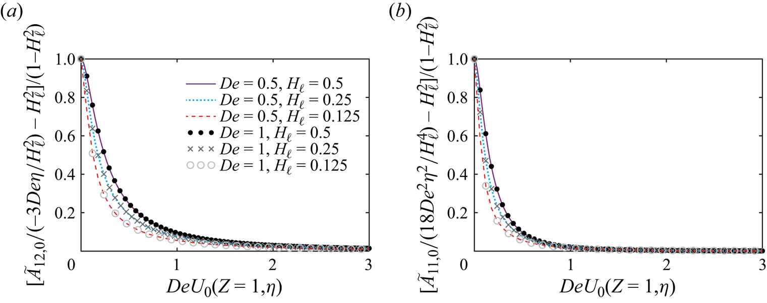
Figure 5. (a,b) Scaled elastic shear and normal stresses at the end of the contraction, ( $a$)
$a$)  $\tilde {A}_{12,0}(Z=1,\eta )/(-3De\eta /H_{\ell }^2)$ and ( $b$)
$b$)  $\tilde {A}_{11,0}(Z=1,\eta )/(18De^2\eta ^2/H_{\ell }^4)$ minus $H_{\ell }^2$, divided by the factor $1-H_{\ell }^2$, as a function of $DeU_{0}(Z=1,\eta )$ for $De=0.5, 1$ and $H_{\ell }=0.125,0.25$ and 0.5. This rescaling leads to an approximate collapse of the results on the single uniform curve for different Deborah numbers and contraction ratios.
5.2. Pressure gradient relaxation in the exit channel
It follows from figure 3(d–f) in the previous subsection that, as  $De$ increases, there is a significant relaxation of the elastic stresses in the exit channel, which occurs over a long distance. Specifically, the elastic stresses relax exponentially over a distance which is proportional to the centreline velocity $(3/2H_{\ell })$ multiplied by the Deborah number $De$ (see (B3)–(B5)). For this reason, a longer downstream section is required at higher $De$.
$De$.
In this subsection, we study the relaxation of the pressure gradient in the downstream section. Substituting  $H(Z)=H_{\ell }$ into (2.19) yields the pressure gradient in the exit channel
 \begin{equation} \frac{\mathrm{d}P}{\mathrm{d}Z}={-}\frac{3(1-\tilde{\beta})}{H_{\ell}^{3}}+\frac{3 \tilde{\beta}}{2De}\int_{0}^{1}(1-\eta^{2})\frac{\partial\tilde{A}_{11,0}}{\partial Z}\mathrm{d}\eta+\frac{3 \tilde{\beta}}{H_{\ell}De}\int_{0}^{1}\eta\tilde{A}_{12,0}\,\mathrm{d}\eta+O(\tilde{\beta}^2).\end{equation}
Noting that in the exit channel  $U_{0}=(3/2H_{\ell })(1-\eta ^{2})$ and $\mathrm {d} U_{0}/\mathrm {d}\eta =-(3/H_{\ell })\eta$, and using the expression for $U_{0}\partial \tilde {A}_{11,0}/\partial Z$ from (B2c), (5.2) can be written as
 \begin{equation} \left(\frac{\mathrm{d}P}{\mathrm{d}Z}+\frac{3}{H_{\ell}^{3}}\right)\frac{1}{\tilde{\beta}}= \frac{3}{H_{\ell}^{3}}-\frac{H_{\ell}}{De^2}\int_{0}^{1}\tilde{A}_{11,0}\,\mathrm{d}\eta-\frac{3 }{H_{\ell}De}\int_{0}^{1}\eta\tilde{A}_{12,0}\,\mathrm{d}\eta,\end{equation}
where the right-hand side is independent of  $\tilde {\beta }$.
We present in figure 6(a) the relaxation of the scaled pressure gradient  $(\mathrm {d}P/\mathrm {d}Z+3/H_{\ell }^3)/\tilde {\beta }$ as a function of the downstream distance $Z_{\ell }$ for $De=0.02,0.2,1$ and 2. Similar to elastic stresses, the scaled pressure gradient relaxes exponentially over the downstream distance, which significantly increases with $De$. Furthermore, we observe a good agreement between the low- and high- $De$ asymptotic solutions (cyan dotted and red dashed lines) and the semi-analytical results (solid lines).

Figure 6. The spatial relaxation of the pressure gradient for the Oldroyd-B fluid in the uniform exit channel of a contraction in the ultra-dilute limit. ( $a$) Scaled pressure gradient $(\mathrm {d}P/\mathrm {d}Z+3/H_{\ell }^3)/\tilde {\beta }$ as a function of the downstream distance $Z_{\ell }$ for $De=0.02,0.2,1$ and 2. ( $b$) Scaled pressure gradient $(\mathrm {d}P/\mathrm {d}Z+3/H_{\ell }^3)/\tilde {\beta }$ as a function of the rescaled downstream distance $2H_{\ell }Z_{\ell }/3De$ in a log $-$linear plot. Solid lines represent the semi-analytical solutions obtained from (5.3) using (B3)–(B5). Cyan dotted lines represent the low- $De$ asymptotic solutions obtained from (5.3) using (B7). Red dashed lines represent the high- $De$ asymptotic solutions obtained from (5.3) using (B9). The green dashed line is $100\exp ({-2H_{\ell }Z_{\ell }/3De})$. All calculations were performed using $H_{\ell }=0.5$.
Recalling that the elastic stresses relax exponentially over a distance proportional to  $(3De/2H_{\ell })$, we replot in figure 6(b) the scaled pressure gradient, (5.3), as a function of the rescaled downstream distance $2H_{\ell }Z_{\ell }/3De$ in a log $-$linear plot. As a result, all curves become parallel to the green dashed line $100\exp ({-2H_{\ell }Z_{\ell }/3De})$, thus confirming that the pressure gradient relaxes over a length scale ${\sim }(3De/2H_{\ell })$, similar to the elastic stresses. More specifically, it follows from figure 6(b) that the downstream distance over which the scaled pressure gradient (PG) decays to 1 % of its maximum value, $L_{1\,\%}^{PG}$, is approximately
 \begin{equation} L_{1\,\%}^{PG}\approx (5.3 \pm 0.5)\times \frac{3De}{2H_{\ell}},\end{equation}
where we obtain that the prefactor  $5.3 \pm 0.5$ is weakly dependent on $De$ throughout the investigated range of Deborah numbers. Equation (5.4) and the scaling $3De/2H_{\ell }$ indicate that, in the exit channel, the appropriate Deborah number is based on the exit height, i.e. $De_{exit}=\lambda q/2h_{\ell }\ell =De/H_{\ell }$.
We note that our estimate of the length of the downstream section, (5.4), is consistent with previous numerical studies on the viscoelastic flows in 2-D abrupt contractions (Debbaut et al. Reference Debbaut, Marchal and Crochet1988; Alves et al. Reference Alves, Oliveira and Pinho2003). Specifically, (5.4) predicts  $L_{1\,\%}^{PG}\approx 239 \pm 23$ for $De_{exit}=De/H_{\ell }=30$, which should be contrasted with 250 of Debbaut et al. (Reference Debbaut, Marchal and Crochet1988), who studied numerically the flow through the planar $4\,{:}\,1$ contraction.
5.3. Pressure drop in the contraction and exit channel
In this subsection, we study the pressure drop across the contraction and the exit channel. First, in figure 7(a) we present the non-dimensional pressure drop  $\Delta P=\Delta p/(\mu _{0}q\ell /2h_{0}^{3})$ in the contraction as a function of $De=\lambda q/(2\ell h_{0})$ for $H_{\ell }=0.5$ and $\tilde {\beta }=0.05$. For further clarification, figure 7(b) shows the first-order contribution $\Delta P_{1}=\Delta p_{1}/(\mu _{0}q\ell /2h_{0}^{3})$ as a function of $De=\lambda q/(2\ell h_{0})$, which is independent of $\tilde {\beta }$. Black dots represent the semi-analytical solution (3.28), cyan dotted lines represent the low- $De$ asymptotic solution (3.32) and red dashed lines represent the high- $De$ asymptotic solution (3.35). Clearly, there is excellent agreement between our low- and high- $De$ asymptotic solutions and the semi-analytical results. We also validate the predictions of our semi-analytical and asymptotic results against the 2-D finite-element simulations with $H_{\ell }=0.5$, $\tilde {\beta }=0.05$ and $\epsilon =0.02$ (grey triangles), showing very good agreement. The details of the numerical implementation in the finite-element software COMSOL Multiphysics are provided in Boyko & Stone (Reference Boyko and Stone2022).

Figure 7. Non-dimensional pressure drop for the Oldroyd-B fluid in a contracting channel in the ultra-dilute limit. ( $a$) Dimensionless pressure drop $\Delta P=\Delta p/(\mu _{0}q\ell /2h_{0}^{3})$ as a function of $De=\lambda q/(2\ell h_{0})$ for $\tilde {\beta }=0.05$. ( $b$) First-order contribution $\Delta P_{1}=\Delta p_{1}/(\mu _{0}q\ell /2h_{0}^{3})$ to the dimensionless pressure drop as a function of $De=\lambda q/(2\ell h_{0})$. Grey triangles in ( $a$) represent the results of the finite-element simulation. Black dots represent the semi-analytical solution (3.28). Cyan dotted lines represent the low- $De$ asymptotic solution (3.32). Red dashed lines represent the high- $De$ asymptotic solution (3.35). All calculations were performed using $H_{\ell }=0.5$.
It is evident that the semi-analytical solution for the pressure drop in the contraction approaches the high- $De$ asymptotic solution for $De\gtrsim 0.4$ and linearly decreases with the Deborah number. First, such an agreement for $De\gg \!\!\!\!\!\!/~1$ is consistent with our results for the elastic stresses, shown in figure 3, and recent results of Hinch et al. (Reference Hinch, Boyko and Stone2024). Second, and more importantly, from the excellent agreement between the semi-analytical results and the high- $De$ asymptotic solution, based on the components of the conformation tensor within the core flow region, we conclude that the viscoelastic boundary layer near the walls makes a negligible contribution to the pressure drop in the contracting channel.
Next, in figure 8(a) we present the non-dimensional pressure drop  $\Delta P_{\ell }$ in the exit channel as a function of $De$ for $H_{\ell }=0.5$, $\tilde {\beta }=0.05$, and $L=50$. For $De=2$, a long exit channel of $L\gtrsim 30$ is required to reach the full relaxation of the elastic stresses and pressure gradient, consistent with (5.4). Figure 8(b) shows the first-order contribution $\Delta P_{\ell,1}$ as a function of $De$, which is independent of $\tilde {\beta }$. In contrast to the total pressure drop $\Delta P_{\ell }$, the first-order contribution $\Delta P_{\ell,1}$ does not depend on $L$, as shown in (4.2), provided that $L$ is sufficiently long so that by the end of the exit channel the elastic stresses have achieved their fully relaxed values (2.16) with $H \equiv H_{\ell }$.

Figure 8. Non-dimensional pressure drop for the Oldroyd-B fluid in the exit channel of a contraction in the ultra-dilute limit. (a) Dimensionless pressure drop  $\Delta P_{\ell }=\Delta p_{\ell }/(\mu _{0}q\ell /2h_{0}^{3})$ as a function of $De=\lambda q/(2\ell h_{0})$ for $\tilde {\beta }=0.05$ and $L=50$. (b) First-order contribution $\Delta P_{\ell,1}=\Delta p_{\ell,1}/(\mu _{0}q\ell /2h_{0}^{3})$ to the dimensionless pressure drop as a function of $De=\lambda q/(2\ell h_{0})$. Black dots represent the semi-analytical solutions (4.1) ( $\Delta P_{\ell }$ in (a)) and (4.2) ( $\Delta P_{\ell,1}$ in (b)). The cyan dotted curve represents the low- $De$ asymptotic solution (4.3). Red dashed lines represent the high- $De$ asymptotic solution (4.4). The inset in (a) shows a comparison of semi-analytical predictions (black dots) and finite-element simulation results (grey triangles) for $\Delta P_{\ell }-\Delta P_{\ell,0}=\tilde {\beta } \Delta P_{\ell,1}$ as a function of $De$ for $\tilde {\beta }=0.05$ and $L=5$. The inset in (b) shows $\Delta P_{\ell }-\Delta P_{\ell,0}=\tilde {\beta } \Delta P_{\ell,1}$ as a function of $De$ for $\tilde {\beta }=0.05$ in range of $1\leq De\leq 10$. All calculations were performed using $H_{\ell }=0.5$.
The inset in figure 8(a) shows a comparison of our semi-analytical predictions (black dots) and finite-element simulation results (grey triangles) for  $\Delta P_{\ell }-\Delta P_{\ell,0}=\tilde {\beta } \Delta P_{\ell,1}$ as a function of $De$ for $H_{\ell }=0.5$, $\tilde {\beta }=0.05$ and $L=5$. We observe excellent agreement between the semi-analytical and numerical results. In addition, the low- $De$ asymptotic solution (cyan dotted curve) accurately captures the numerical results for $De<0.05$ and indicates that the pressure drop in the exit channel scales as $De^3$ for $De\ll 1$.
Similar to the contraction, the pressure drop in the exit channel linearly decreases with  $De$ for $De\gtrsim 0.3$, as shown in figure 8. While our semi-analytical solution linearly diminishes with the slope of $-36/5$, as predicted by the high- $De$ asymptotic solution (red dashed lines), there is an offset between the two results for $\tilde {\beta } \Delta P_{\ell,1}$. In particular, for $De=0.4$, we have a non-negligible relative error of approximately 30 %. However, the inset in figure 8(b) shows that as $De$ increases, the agreement between our semi-analytical solution and the high- $De$ asymptotic prediction significantly improves, resulting in relative errors of only approximately 5 % and 1 % for $De=2$ and $De=10$, respectively.
We note that our theoretical approach, based on the ultra-dilute limit, allows us to study the behaviour of the elastic stresses and pressure drop at arbitrary values of  $De$. In particular, we can predict the behaviour in the high-Deborah-number regime, for example, $De=2$ and even $De=10$, which we are currently unable to access via finite-element simulations. Note, however, that we have assumed steady flows, so further investigation would be required to assess whether there might be flow instabilities at higher $De$.
$De$.
5.4. Different contributions to the pressure drop in the contraction and exit channel
In the previous subsection, we observed a monotonic reduction in the dimensionless pressure drop with increasing  $De$ for an Oldroyd-B fluid flowing through the contraction and exit channel (figures 7 and 8). To understand the source of such pressure drop reduction, we elucidate the relative importance of elastic contributions to the pressure drop.
The elastic contributions to the non-dimensional pressure drop across the contraction and exit channel, scaled by  $\tilde {\beta }$, as a function of $De$ are shown in figures 9(a) and 9(b), respectively. Black circles and grey dots represent the elastic shear and normal stress contributions obtained from the semi-analytical solutions (3.28) and (4.1). Cyan dotted and purple curves represent the elastic shear and normal stress contributions obtained from the low- $De$ asymptotic solutions (3.32) and (4.3). Red and black dashed lines represent the elastic shear and normal stress contributions obtained from the high- $De$ asymptotic solutions (3.35) and (4.4). As expected based on our previous results, we observe excellent agreement between our low- and high- $De$ asymptotic solutions and the semi-analytical predictions.
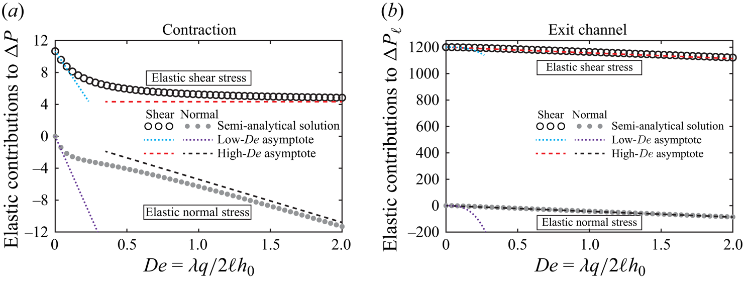
Figure 9. Elastic contributions to the non-dimensional pressure drop of the Oldroyd-B fluid, scaled by  $\tilde {\beta }$, in (a) the contraction and (b) the exit channel in the ultra-dilute limit. Black circles and grey dots represent the semi-analytical solutions (3.28) (contraction) and (4.1) (exit channel) for elastic shear and normal stress contributions. Cyan dotted and purple curves represent the low- $De$ asymptotic solutions (3.32) (contraction) and (4.3) (exit channel) for elastic shear and normal stress contributions. Red and black dashed lines represent the high- $De$ asymptotic solutions (3.35) (contraction) and (4.4) (exit channel) for elastic shear and normal stress contributions. All calculations were performed using $H_{\ell }=0.5$ and $L=50$.
The first main source for the pressure drop reduction is the elastic normal stress contribution, which linearly decreases with  $De$ in the contraction and exit channel at low and high Deborah numbers. As noted by Hinch et al. (Reference Hinch, Boyko and Stone2024), this is because the elastic normal stresses, which correspond to the tension in the streamlines, are higher at the end of the contraction (exit channel) compared with the beginning of the contraction (exit channel). These higher elastic normal stresses pull the fluid along and thus require less pressure to push.
The second main source for the pressure drop reduction is the decrease of elastic shear stress contribution with  $De$ due to the long time (or long distance) required for the elastic shear stresses to approach their eventual relaxed values far downstream. As a result, the elastic shear stresses are lower than the fully relaxed value $\tilde {A}_{12}=-3De\eta /H_{\ell }^{2}$ (see figure 3), and their contribution to the pressure drop is smaller than the steady Poiseuille value of $3\tilde {\beta }\int _{0}^{1}H(Z)^{-3}\,\mathrm {d}Z$ (contraction) and $3\tilde {\beta }L/H_{\ell }^3$ (exit channel), thus reducing the pressure drop. At low Deborah numbers, such a decrease scales as $De$ and $De^3$ for a smooth contraction and exit channel, respectively. However, at high Deborah numbers, it approaches a constant asymptotic value of $3\tilde {\beta }\int _{0}^{1}H(Z)^{-1}\,\mathrm {d}Z$ for the contraction. For the exit channel, $\Delta P_{\ell,1}^{SS}$ linearly depends on the Deborah number since the relaxation of the elastic shear stresses occurs over the distance $L$, which scales linearly with $De$, as shown in (5.4).
6. Concluding remarks
In this work, we applied the lubrication approximation and considered the ultra-dilute limit to study the flow of an Oldroyd-B fluid in arbitrarily shaped contracting channels. Specifically, we exploited the one-way coupling between the parabolic velocity and polymer conformation tensor in the ultra-dilute limit to derive closed-form expressions for the microstructure deformation and the flow rate–pressure drop relation for arbitrary values of the Deborah number. We provided analytical expressions for the conformation tensor and the  $q-\Delta p$ relation in the low- and high-Deborah-number limits for the contraction and exit channels, complementing the asymptotic results of Boyko & Stone (Reference Boyko and Stone2022) and the analysis of Hinch et al. (Reference Hinch, Boyko and Stone2024) at any concentration. We further analysed the viscoelastic boundary layer of thickness $O(De^{-1})$, existing near the walls at high Deborah numbers, and derived the boundary-layer asymptotic solutions. We validated our semi-analytical and asymptotic results for the pressure drop in the smooth contraction and exit channels with 2-D finite-element numerical simulations and found excellent agreement.
For both contraction and exit channels, the pressure drop of an Oldroyd-B fluid monotonically decreases with increasing  $De$ and scales linearly with $De$ at high Deborah numbers, as shown in figures 7 and 8. We identified two mechanisms for such pressure drop reduction (see figure 9). The first is higher elastic normal stresses at the end of the contraction and exit channels, relative to the corresponding entry values, that pull the fluid along and thus require less pressure to push. The second source for the pressure drop reduction is because, once perturbed from their upstream values, the elastic shear stresses require a long distance to approach their new downstream fully relaxed values, as shown in figure 3, so again reducing the pressure drop.
Our theoretical approach, which relies on lubrication theory and the ultra-dilute limit, allows us to study the behaviour of the elastic stresses and pressure drop of an Oldroyd-B fluid at arbitrary values of  $De$. Our theory is not restricted to the case of 2-D contracting channels and can be utilized to study different slowly varying geometries, such as expansions and constrictions. The approach can also be extended to axisymmetric geometries. Furthermore, the theoretical framework we presented enables us to access sufficiently high Deborah numbers, which are difficult and sometimes impossible to study via numerical simulations due to the high-Weissenberg-number problem (Owens & Phillips Reference Owens and Phillips2002; Alves et al. Reference Alves, Oliveira and Pinho2021). We, therefore, believe that our analytical and semi-analytical results for the ultra-dilute limit are of fundamental importance as they may serve for simulation validation.
Finally, we note that our theoretical predictions for the pressure drop reduction of an Oldroyd-B fluid in a contraction are consistent with the previous numerical reports on 2-D abruptly contracting geometries (Aboubacar, Matallah & Webster Reference Aboubacar, Matallah and Webster2002; Alves et al. Reference Alves, Oliveira and Pinho2003; Binding et al. Reference Binding, Phillips and Phillips2006; Aguayo, Tamaddon-Jahromi & Webster Reference Aguayo, Tamaddon-Jahromi and Webster2008). However, these predictions are opposite to the experiments showing a nonlinear increase in the pressure drop with  $De$ for the flow of a Boger fluid through abrupt axisymmetric contraction–expansion and contraction geometries (Rothstein & McKinley Reference Rothstein and McKinley1999, Reference Rothstein and McKinley2001; Nigen & Walters Reference Nigen and Walters2002; Sousa et al. Reference Sousa, Coelho, Oliveira and Alves2009). As noted by Alves et al. (Reference Alves, Oliveira and Pinho2003) and Hinch et al. (Reference Hinch, Boyko and Stone2024), this discrepancy might be attributed to the lack of dissipative effects in the Oldroyd-B model. Thus, as a future research direction, it is interesting to study more complex constitutive equations, such as a finitely extensible nonlinear elastic (FENE) model introduced by Chilcott & Rallison (Reference Chilcott and Rallison1988) (FENE-CR) and a finitely extensible nonlinear elastic model with the Peterlin approximation (FENE-P), that incorporate dissipation and additional microscopic features of polymer solutions and understand how these features affect the pressure drop. We anticipate that even for a more complex constitutive model, the theoretical framework presented here will enable the development of a simplified, reduced-order theory, allowing us to study the behaviour at non-small Deborah numbers.
Funding
E.B. acknowledges the support by grant no. 2022688 from the US-Israel Binational Science Foundation (BSF). H.A.S. acknowledges the support from grant no. CBET-2246791 from the United States National Science Foundation (NSF).
Declaration of interests
The authors report no conflict of interest.
Appendix A. Orthogonal curvilinear coordinates for a slowly varying geometry
In this appendix, we provide additional details for orthogonal curvilinear coordinates for a slowly varying geometry used in our theoretical analysis. We consider a slowly spatially varying channel with a given shape  $h$ that varies on the length scale $\ell$, so that $h=h(z/\ell )=h_0 H(Z)$. We transform the Cartesian coordinates ( $Z,Y$) to curvilinear coordinates ( $\xi,\eta$) with the mapping
 \begin{equation} \xi=Z+\epsilon^2 Q(Z,Y),\quad\eta=\frac{Y}{H(Z)},\end{equation}
where  $Z=z/\ell$, $Y=y/h_0$ and $Q$ is an unknown function yet to be determined. Note that, in the lubrication limit, the orthogonal coordinate $\xi$ (scaled by $\ell$) is nearly in the $z$-direction.
We find  $Q(Z,Y)$ by requiring that the curvilinear coordinates ( $\xi,\eta$) are orthogonal, i.e. $\boldsymbol {\nabla }\xi \boldsymbol {\cdot }\boldsymbol {\nabla }\eta =0$. Using the relations
 \begin{gather} \boldsymbol{\nabla}\xi=\left[\epsilon\frac{\partial \xi}{\partial Z},\frac{\partial\xi}{\partial Y}\right]=\left[\epsilon\left(1+\epsilon^{2}\frac{\partial Q}{\partial Z}\right),\epsilon^{2}\frac{\partial Q}{\partial Y}\right], \end{gather}
 \begin{gather}\boldsymbol{\nabla}\eta=\left[\epsilon\frac{\partial\eta}{\partial Z},\frac{\partial\eta}{\partial Y}\right]=\left[-\epsilon\frac{YH'(Z)}{H(Z)^{2}},\frac{1}{H(Z)}\right], \end{gather}
we obtain
 \begin{equation} \boldsymbol{\nabla}\xi\boldsymbol{\cdot}\boldsymbol{\nabla}\eta=\frac{\epsilon^{2}}{H(Z)}\left[-\left(1+\epsilon^{2}\frac{\partial Q}{\partial Z}\right)\frac{Y H'(Z)}{H(Z)}+\frac{\partial Q}{\partial Y}\right].\end{equation}
Therefore,  $\boldsymbol {\nabla }\xi \boldsymbol {\cdot }\boldsymbol {\nabla }\eta =O(\epsilon ^{4})$ provided we set
 \begin{equation} \frac{\partial Q}{\partial Y}=\frac{YH'(Z)}{H(Z)}\Rightarrow Q(Z,Y)={-}\frac{1}{2}\frac{H'(Z)}{H(Z)}(H(Z)^{2}-Y^{2}),\end{equation}
where without loss of generality, we choose  $Q\equiv 0$ on $Y=H(Z)$. Hence, the orthogonal curvilinear coordinates ( $\xi,\eta$) are
 \begin{equation} \xi=Z-\frac{1}{2}\epsilon^{2}\frac{H'(Z)}{H(Z)}(H(Z)^{2}-Y^{2})+O(\epsilon^{4}), \quad\eta=\frac{Y}{H(Z)}.\end{equation}
Using (A5a,b), the inverse transformation is (see also Hinch et al. Reference Hinch, Boyko and Stone2024)
 \begin{gather} Z=\xi+\tfrac{1}{2}\epsilon^{2} H'(\xi)H(\xi)(1-\eta^{2})+O(\epsilon^{4})=\xi+\tfrac{1}{4}(H(\xi)^{2})'(1-\eta^{2}) + O(\epsilon^{4}), \end{gather}
 \begin{gather}Y(\xi,\eta)=\eta H(\xi), \end{gather}
where evaluating  $H(\xi )$ rather than $H(Z)$ introduces a relative error of $O(\epsilon ^{2})$.
In what follows, it is also convenient to use the dimensional form of the transformation (A6), given as
 \begin{equation} z=\bar{\xi}+\frac{1}{2}\epsilon h_0 \frac{\mathrm{d}H(\xi)}{\mathrm{d}\xi} H(\xi)(1-\eta^{2})+O(\epsilon^{4}), \quad y=\eta h_0 H(\xi ),\end{equation}
where we have defined the dimensional coordinate  $\bar {\xi }=\xi \ell$.
A.1. Curvilinear orthonormal basis vectors
The expressions for the curvilinear orthonormal basis vectors  $\boldsymbol {e}_{\xi }$ and $\boldsymbol {e}_{\eta }$ in terms of $\boldsymbol {e}_{z}$ and $\boldsymbol {e}_{y}$ are obtained from
 \begin{equation} \boldsymbol{e}_{\xi}=\frac{\partial\boldsymbol{x}}{\partial\bar{\xi}}\frac{1}{\left| \partial\boldsymbol{x}/\partial\bar{\xi}\right|},\quad \boldsymbol{e}_{\eta}=\frac{\partial\boldsymbol{x}}{\partial\eta}\frac{1}{\left|\partial\boldsymbol{x}/\partial\eta\right|},\end{equation}
where using (A7a,b), we have
 \begin{gather} \frac{\partial\boldsymbol{x}}{\partial\bar{\xi}}=\left(\frac{\partial z}{\partial\bar{\xi}},\frac{\partial y}{\partial\bar{\xi}}\right)=\left(1+O(\epsilon^{2}),h_{0}\frac{\mathrm{d}H(\xi)}{\mathrm{d}\bar{\xi}}\eta\right)\underset{\bar{\xi}=\ell\xi}=\left(1+O(\epsilon^{2}),\epsilon\frac{\mathrm{d}H(\xi)}{\mathrm{d}\xi}\eta\right), \end{gather}
 \begin{gather}\frac{\partial\boldsymbol{x}}{\partial\eta}=\left(\frac{\partial z}{\partial \eta},\frac{\partial y}{\partial \eta }\right)=\left(-\epsilon h_{0}\frac{\mathrm{d}H(\xi)}{\mathrm{d}\xi}H(\xi)\eta,h_{0}H(\xi)\right), \end{gather}
and  $h_{\xi }=|\partial \boldsymbol {x}/\partial \bar {\xi }|\approx 1$ and $h_{\eta }=|\partial \boldsymbol {x}/\partial \eta |\approx h_{0}H(\xi )=h(\bar {\xi }/ \ell )$ are the metric coefficients (or scale factors) in the $\xi$- and $\eta$-directions, respectively, with small corrections of $O(\epsilon ^{2})$.
Substituting (A9) into (A8a,b), we obtain
 \begin{equation} \boldsymbol{e}_{\xi}\approx\boldsymbol{e}_{z}+\epsilon H'(\xi)\eta\boldsymbol{e}_{y}, \quad \boldsymbol{e}_{\eta}\approx{-}\epsilon H'(\xi)\eta\boldsymbol{e}_{z}+\boldsymbol{e}_{y}.\end{equation}
A.2. Velocity and conformation tensor in Cartesian and curvilinear coordinates
The velocity field and the conformation tensor can be expressed either in Cartesian or curvilinear coordinates. Specifically, the velocity  $\boldsymbol {u}=u_z\boldsymbol {e}_{z}+u_y\boldsymbol {e}_{y}$ in Cartesian coordinates is related to the velocity $\boldsymbol {u}=u\boldsymbol {e}_{\xi }+\upsilon \boldsymbol {e}_{\eta }$ in curvilinear coordinates through (Brand Reference Brand1947)
 \begin{equation} \left(\begin{array}{c} u_{z}\\ u_{y} \end{array}\right)=\boldsymbol{\mathsf{M}}\boldsymbol{\cdot}\left(\begin{array}{c} u\\ \upsilon \end{array}\right),\end{equation}
where  $\boldsymbol{\mathsf{M}}$ is the coordinate transformation matrix obtained from (A10a,b) and given as
 \begin{equation} \boldsymbol{\mathsf{M}}=\left(\begin{array}{cc} 1 & -\epsilon H'(\xi)\eta\\ \epsilon H'(\xi)\eta & 1 \end{array}\right).\end{equation}
We introduce non-dimensional velocity components in curvilinear coordinates, similar to the non-dimensionalization (2.5a),
 \begin{equation} U=\frac{u}{u_{c}},\quad V=\frac{\upsilon}{\epsilon u_{c}}.\end{equation}
Using (A11)–(A13a,b) provides the relations between non-dimensional velocity components in different coordinates
 \begin{equation} U_{z}=U-\epsilon^{2}\eta H'(\xi) V, \quad U_{y}=\eta H'(\xi) U+V.\end{equation}
While velocity in the  $z$- and $\xi$-directions are the same, albeit to a $O(\epsilon ^{2})$ correction, the velocity in the $y$-direction is greater by $\eta H'(\xi ) U$ than the velocity in the $\eta$-direction.
Similarly, the conformation tensor  $\boldsymbol{\mathsf{A}}=A_{zz}\boldsymbol {e}_{z}\boldsymbol {e}_{z}+A_{zy}(\boldsymbol {e}_{z}\boldsymbol {e}_{y}+ \boldsymbol {e}_{y}\boldsymbol {e}_{z})+A_{yy}\boldsymbol {e}_{y}\boldsymbol {e}_{y}$ in Cartesian coordinates is related to the conformation tensor $\boldsymbol{\mathsf{A}}=A_{11}\boldsymbol {e}_{\xi }\boldsymbol {e}_{\xi }+A_{12}(\boldsymbol {e}_{\xi } \boldsymbol {e}_{\eta }+\boldsymbol {e}_{\eta }\boldsymbol {e}_{\xi })+A_{22}\boldsymbol {e}_{\eta } \boldsymbol {e}_{\eta }$ in curvilinear coordinates through (Brand Reference Brand1947)
 \begin{equation} \left(\begin{array}{cc} A_{zz} & A_{zy}\\ A_{yz} & A_{yy} \end{array}\right)=\boldsymbol{\mathsf{M}}\boldsymbol{\cdot}\left(\begin{array}{cc} A_{11} & A_{12}\\ A_{21} & A_{22} \end{array}\right)\boldsymbol{\cdot}\boldsymbol{\mathsf{M}}^{\mathrm{T}}.\end{equation}
Next, we define scaled  $\tilde {A}_{11}$, $\tilde {A}_{12}$ and $\tilde {A}_{22}$ in curvilinear coordinates, similar to the non-dimensionalization (2.5c)
 \begin{equation} \tilde{A}_{11}=\epsilon^{2}A_{11},\quad\tilde{A}_{12}=\epsilon A_{12},\quad\tilde{A}_{22}=A_{22}.\end{equation}
Finally, using (A12) and (A15)–(A16), we obtain the relations between conformation tensor components in different coordinates
 \begin{gather} \tilde{A}_{zz}=\tilde{A}_{11}+O(\epsilon^{2}), \end{gather}
 \begin{gather}\tilde{A}_{zy}=\tilde{A}_{12}+\eta H'(\xi)\tilde{A}_{11}+O(\epsilon^{2}), \end{gather}
 \begin{gather}\tilde{A}_{yy}=\tilde{A}_{22}+2\eta H'(\xi)\tilde{A}_{12}+\eta^2 (H'(\xi))^2\tilde{A}_{11}+O(\epsilon^{2}). \end{gather}
Appendix B. Low-$\tilde {\beta }$ lubrication analysis in the exit channel: detailed derivation

We here provide details of the derivation of closed-form expressions for the conformation tensor and the pressure drop in the uniform exit channel for  $\tilde {\beta }\ll 1$.
B.1. Velocity, conformation and pressure drop in the exit channel at the leading order in $\tilde {\beta }$

The velocity field and pressure drop in the exit channel at the leading order in  $\tilde {\beta }$ are
 \begin{equation} U_{0}=\frac{3}{2}\frac{1}{H_{\ell}}(1-\eta^{2}),\quad V_{0}\equiv0,\quad \Delta P_{\ell,0}=\frac{3L}{H_{\ell}^{3}}.\end{equation}
As expected, (B1) simply represents the solution for the velocity and pressure drop of a Newtonian fluid with a constant viscosity  $\mu _0$ flowing in a straight channel of (non-dimensional) height $H_{\ell }$ and length $L$.
$L$.
Substituting (B1a) into (3.6), we obtain the governing equations for the conformation tensor components in the exit channel at the leading order in  $\tilde {\beta }$
 \begin{gather} U_{0}\frac{\partial\tilde{A}_{22,0}}{\partial Z}={-}\frac{1}{De}(\tilde{A}_{22,0}-1), \end{gather}
 \begin{gather}U_{0}\frac{\partial\tilde{A}_{12,0}}{\partial Z}-\frac{1}{H_{\ell}}\frac{\mathrm{d} U_{0}}{\mathrm{d}\eta}\tilde{A}_{22,0}={-}\frac{1}{De}\tilde{A}_{12,0}, \end{gather}
 \begin{gather}U_{0}\frac{\partial\tilde{A}_{11,0}}{\partial Z}-\frac{2}{H_{\ell}}\frac{\mathrm{d} U_{0}}{\mathrm{d}\eta}\tilde{A}_{12,0}={-}\frac{1}{De}\tilde{A}_{11,0}. \end{gather}
Equations (B2), similar to (3.6), represent a set of one-way coupled first-order semi-linear partial differential equations that can be solved first for  $\tilde {A}_{22,0}$, followed by $\tilde {A}_{12,0}$ and then for $\tilde {A}_{11,0}$. The solution of these equations is
 \begin{gather} \tilde{A}_{22,0}=1+(\tilde{A}_{22,0}^{ref}(\eta)-1)\exp({-2H_{\ell}Z_{\ell}/[3De(1-\eta^{2})]}),\end{gather}
 \begin{gather}
\tilde{A}_{12,0}={-}\frac{3De}{H_{\ell}^{2}}\eta+\exp({-2H_{\ell}Z_{\ell}/[3De(1-\eta^{2})]})
\left[\vphantom{\left. +\,\frac{3De}{H_{\ell}^{2}}\eta-\frac{2\eta(\tilde{A}_{22,0}^{ref}(
\eta)-1)Z_{\ell}}{H_{\ell}(1-\eta^{2})}\right]}\tilde{A}_{12,0}^{ref}(\eta)\right.\nonumber\\ \left. +\,\frac{3De}{H_{\ell}^{2}}\eta-\frac{2\eta(\tilde{A}_{22,0}^{ref}(
\eta)-1)Z_{\ell}}{H_{\ell}(1-\eta^{2})}\right],\end{gather}
\begin{gather}
\tilde{A}_{12,0}={-}\frac{3De}{H_{\ell}^{2}}\eta+\exp({-2H_{\ell}Z_{\ell}/[3De(1-\eta^{2})]})
\left[\vphantom{\left. +\,\frac{3De}{H_{\ell}^{2}}\eta-\frac{2\eta(\tilde{A}_{22,0}^{ref}(
\eta)-1)Z_{\ell}}{H_{\ell}(1-\eta^{2})}\right]}\tilde{A}_{12,0}^{ref}(\eta)\right.\nonumber\\ \left. +\,\frac{3De}{H_{\ell}^{2}}\eta-\frac{2\eta(\tilde{A}_{22,0}^{ref}(
\eta)-1)Z_{\ell}}{H_{\ell}(1-\eta^{2})}\right],\end{gather} \begin{align} \tilde{A}_{11,0}&=\frac{18De^{2}}{H_{\ell}^{4}}\eta^{2}+\exp({-2H_{\ell}Z_{\ell}/[3De(1-\eta^{2})]}) \left[ \tilde{A}_{11,0}^{\mathrm{ref}}(\eta)-\frac{18De^{2}}{H_{\ell}^{4}}\eta^{2} \right. \nonumber\\ &\quad \left. +\frac{4\eta^{2}(\tilde{A}_{22,0}^{ref}(\eta)-1)Z_{\ell}^{2}}{H_{\ell}^{2}(1-\eta^{2})^{2}} -\frac{4\eta Z_{\ell}[3De\eta+H_{\ell}^{2}\tilde{A}_{12,0}^{ref}(\eta)]}{H_{\ell}^{3}(1-\eta^{2})} \right], \end{align}
where  $Z_{\ell }=Z-1$ and $\tilde {A}_{22,0}^{ref}(\eta )=\tilde {A}_{22,0}(Z=1,\eta )$, $\tilde {A}_{12,0}^{ref}(\eta )=\tilde {A}_{12,0}(Z=1,\eta )$ and $\tilde {A}_{11,0}^{ref}(\eta )=\tilde {A}_{11,0}(Z=1,\eta )$ are the reference distributions of the conformation tensor components at the outlet ( $Z=1$) of the non-uniform channel that can be obtained from (3.8), (3.9) and (3.10).
We note that, under the assumption of a fully developed flow in the entire exit channel so that  $U(\eta )=(3/2H_{\ell })(1-\eta ^{2})$, the governing equations for the conformation tensor components (B2) and their solution (B3)–(B5) are valid not only at $O(\tilde {\beta }^{0})$ but for arbitrary values of $\tilde {\beta }$.
Finally, we note that the components of the conformation tensor at the walls of the exit channel  $(\eta =\pm 1)$ are given in (3.12), with $H(Z)\equiv H_{\ell }$. Thus, the conformation tensor components at the walls of the exit channel attain their fully relaxed values without spatial development.
B.1.1. Conformation tensor in the exit channel at low $De$ numbers

At low Deborah numbers, we use (3.13) to obtain the reference distributions of the conformation tensor components at the beginning of the exit channel
 \begin{gather} \tilde{A}_{22,0}^{ref}(\eta)=1-\frac{9De^{2}H''(1)}{2H_{\ell}^{3}}(1-\eta^{2})^{2}, \end{gather}
 \begin{gather}\tilde{A}_{12,0}^{ref}(\eta)={-}\frac{3De}{H_{\ell}^{2}}\eta+\frac{81De^{3}H''(1)}{2H_{\ell}^{5}}\eta(1-\eta^{2})^{2}, \end{gather}
 \begin{gather}\tilde{A}_{11,0}^{ref}(\eta)=\frac{18De^{2}}{H_{\ell}^{4}}\eta^{2}-\frac{486De^{4}H''(1)}{H_{\ell}^{7}}\eta^{2}(1-\eta^{2})^{2}, \end{gather}
where, for a smooth geometry, we have assumed that  $H'(1)=H'''(1)=0$.
Substituting (B6) into (B3), we obtain explicit expressions for the spatial relaxation of the conformation tensor components in the exit channel for  $De\ll 1$
 \begin{equation} \tilde{A}_{22,0}=1-\frac{9De^{2}H''(1)}{2H_{\ell}^{3}}(1-\eta^{2})^{2}\exp({-2H_{\ell}Z_{\ell}/[3De(1-\eta^{2})]}),\end{equation}
 \begin{align} \tilde{A}_{12,0}&={-}\frac{3De}{H_{\ell}^{2}}\eta\nonumber\\ &\quad+\frac{9De^{2}H''(1)}{H_{\ell}^{4}} \eta(1-\eta^{2})\exp({-2H_{\ell}Z_{\ell}/[3De(1-\eta^{2})]}) \left[\frac{9De}{2H_{\ell}}(1-\eta^{2})+Z_{\ell}\right], \end{align}
 \begin{align} \tilde{A}_{11,0}&=\frac{18De^{2}}{H_{\ell}^{4}}\eta^{2}-\frac{18De^{2}H''(1)}{H_{\ell}^{5}} \eta^{2}\exp({-2H_{\ell}Z_{\ell}/[3De(1-\eta^{2})]})\left[ \frac{27De^{2}}{H_{\ell}^{2}}(1-\eta^{2})^{2} \right. \nonumber\\ &\quad + \left.Z_{\ell}^{2} +\frac{9 De }{H_{\ell}}Z_{\ell}(1-\eta^{2})\right]. \end{align}
B.1.2. Conformation tensor in the exit channel at high $De$ numbers

From (3.15), (3.17) and (3.19) it follows that the reference distributions of the conformation tensor components at the beginning of the exit channel within the core flow region in the high- $De$ limit are
 \begin{equation} \tilde{A}_{22,0}^{ref}(\eta)=H_{\ell}^{2},\quad\tilde{A}_{12,0}^{ref}(\eta)={-}3De\eta,\quad \tilde{A}_{11,0}^{ref}(\eta)=\frac{18De^{2}}{H_{\ell}^{2}}\eta^{2}.\end{equation}
Substituting (B8) into (B3) provides expressions for the spatial relaxation of the conformation tensor components in the exit channel for  $De\gg 1$
 \begin{gather} \tilde{A}_{22,0}=1+(H_{\ell}^{2}-1)\exp({-2H_{\ell}Z_{\ell}/[3De(1-\eta^{2})]}), \end{gather}
 \begin{gather}\tilde{A}_{12,0}={-}\frac{3De\eta}{H_{\ell}^{2}}+\exp({-2H_{\ell}Z_{\ell}/[3De(1-\eta^{2})]}) \left[{-}3De\eta+\frac{3De\eta}{H_{\ell}^{2}}+\frac{2\eta(1-H_{\ell}^{2})Z_{\ell}}{H_{\ell}(1-\eta^{2})}\right], \end{gather}
 \begin{align} \tilde{A}_{11,0}&=\frac{18De^{2}\eta^{2}}{H_{\ell}^{4}}+\exp({-2H_{\ell}Z_{\ell}/[3De(1-\eta^{2})]}) \left[ \frac{18De^{2}\eta^{2}}{H_{\ell}^{2}}-\frac{18De^{2}\eta^{2}}{H_{\ell}^{4}}\right. \nonumber\\ &\quad \left. +\frac{4\eta^{2}(H_{\ell}^{2}-1)Z_{\ell}^{2}}{H_{\ell}^{2}(1-\eta^{2})^{2}} -\frac{12De\eta^{2}Z_{\ell}(1-H_{\ell}^{2})}{H_{\ell}^{3}(1-\eta^{2})} \right]. \end{align}
B.2. Pressure drop in the exit channel at the first order in $\tilde {\beta }$

Using (2.21) and (3.27), the expressions for the pressure drop at  $O(\tilde {\beta })$, $\Delta P_{\ell, 1}$ and the total pressure drop in the exit channel up to $O(\tilde {\beta })$, $\Delta P_{\ell }$, are
 \begin{equation} \Delta P_{\ell, 1}={-}\frac{3L}{H_{\ell}^{3}}+\frac{3}{2De}\int_{0}^{1}(1-\eta^{2})\left[\tilde{A}_{11,0}\right]_{ Z_{\ell}=L}^{Z_{\ell}=0}\,\mathrm{d}\eta + \frac{3}{DeH_{\ell}}\int_{0}^{1}\eta\left[\int_{L}^{0}\tilde{A}_{12,0}\,\mathrm{d}Z_{\ell}\right]\mathrm{d}\eta,\end{equation}
and
 \begin{equation} \Delta
P_{\ell}=\underset{\textit{Solvent stress}}{\underbrace{(1-\tilde{\beta})\frac{3L}{H_{\ell}^{3}}}}+\underset{\textit{Elastic normal stress}}
{\underbrace{\frac{3\tilde{\beta}}{2De}\int_{0}^{1}(1\!-\!\eta^{2})\left[\tilde{A}_{11,0}\right]_{Z_{\ell}=L}^{Z_{\ell}\!=\!0}\,\mathrm{d}\eta}}
+\underset{\textit{Elastic shear stress}}{\underbrace{\frac{3\tilde{\beta}}{DeH_{\ell}}\int_{0}^{1}\eta
\left[\int_{L}^{0}\tilde{A}_{12,0}\,\mathrm{d}Z_{\ell}\right]\mathrm{d}\eta}},\end{equation}
\begin{equation} \Delta
P_{\ell}=\underset{\textit{Solvent stress}}{\underbrace{(1-\tilde{\beta})\frac{3L}{H_{\ell}^{3}}}}+\underset{\textit{Elastic normal stress}}
{\underbrace{\frac{3\tilde{\beta}}{2De}\int_{0}^{1}(1\!-\!\eta^{2})\left[\tilde{A}_{11,0}\right]_{Z_{\ell}=L}^{Z_{\ell}\!=\!0}\,\mathrm{d}\eta}}
+\underset{\textit{Elastic shear stress}}{\underbrace{\frac{3\tilde{\beta}}{DeH_{\ell}}\int_{0}^{1}\eta
\left[\int_{L}^{0}\tilde{A}_{12,0}\,\mathrm{d}Z_{\ell}\right]\mathrm{d}\eta}},\end{equation}
where  $\tilde {A}_{11,0}$ and $\tilde {A}_{12,0}$ are given in (B4) and (B5) and $[\tilde {A}_{11,0}]_{Z_{\ell }=L}^{Z_{\ell }=0}=\tilde {A}_{11,0}(Z_{\ell }=0,\eta )-\tilde {A}_{11,0}(Z_{\ell }=L,\eta )$. The three terms on the right-hand side of (B11) represent, respectively, the Newtonian solvent stress contribution, the elastic normal stress contribution and the elastic shear stress contribution to the pressure drop.
It is possible to express the first-order contribution  $\Delta P_{\ell, 1}$ in terms of the difference between the conformation tensor components at the beginning and end of the exit channel. First, integrating (B2a) and (B2b) with respect to $Z_{\ell }$ from $L$ to 0, we obtain
 \begin{gather} U_{0}\left[\tilde{A}_{22,0}\right]_{Z_{\ell}=L}^{Z_{\ell}=0}={-}\frac{1}{De}\int_{L}^{0}(\tilde{A}_{22,0}-1)\,\mathrm{d}Z_{\ell}, \end{gather}
 \begin{gather}U_{0}\left[\tilde{A}_{12,0}\right]_{Z_{\ell}=L}^{Z_{\ell}=0}-\frac{1}{H_{\ell}}\frac{\mathrm{d} U_{0}}{\mathrm{d}\eta}\int_{L}^{0}\tilde{A}_{22,0}\,\mathrm{d}Z_{\ell}={-}\frac{1}{De}\int_{L}^{0}\tilde{A}_{12,0}\,\mathrm{d}Z_{\ell}. \end{gather}
Substituting (B12) into (B13) yields
 \begin{equation} U_{0}\left[\tilde{A}_{12,0}\right]_{Z_{\ell}=L}^{Z_{\ell}=0}+\frac{De}{H_{\ell}}\frac{\mathrm{d} U_{0}}{\mathrm{d}\eta}U_{0}\left[\tilde{A}_{22,0}\right]_{Z_{\ell}=L}^{Z_{\ell}=0}+\frac{L}{H_{\ell}}\frac{\mathrm{d} U_{0}}{\mathrm{d}\eta}={-}\frac{1}{De}\int_{L}^{0}\tilde{A}_{12,0}\,\mathrm{d}Z_{\ell}.\end{equation}
Thus, using (B14), the last term on the right-hand side of (B11) can be expressed as
 \begin{align} \frac{3}{DeH_{\ell}}\int_{0}^{1}\eta\left[\int_{L}^{0}\tilde{A}_{12,0}\mathrm{d}Z_{\ell}\right]\mathrm{d}\eta&={-}\frac{9}{2H_{\ell}^2}\int_{0}^{1}\eta(1-\eta^2)\left[\tilde{A}_{12,0}\right]_{Z_{\ell}=L}^{Z_{\ell}=0}\,\mathrm{d}\eta \nonumber\\ &\quad +\frac{27De}{2H_{\ell}^{4}}\int_{0}^{1}\eta^2(1-\eta^2)\left[\tilde{A}_{22,0}\right]_{Z_{\ell}=L}^{Z_{\ell}=0}\, \mathrm{d}\eta+\frac{3L}{H_{\ell}^3}. \end{align}
Substituting (B15) into (B11) provides the alternative expression for  $\Delta P_{\ell,1}$
 \begin{align} \Delta P_{\ell,1}&=\frac{3}{2De}\int_{0}^{1}(1-\eta^{2})\left[\tilde{A}_{11,0}\right]_{Z_{\ell}=L}^{Z_{\ell}=0}\, \mathrm{d}\eta -\frac{9}{2H_{\ell}^2}\int_{0}^{1}\eta(1-\eta^2)\left[\tilde{A}_{12,0}\right]_{Z_{\ell}=L}^{Z_{\ell}=0}\,\mathrm{d}\eta \nonumber\\ &\quad +\frac{27De}{2H_{\ell}^{4}}\int_{0}^{1}\eta^2(1-\eta^2)\left[\tilde{A}_{22,0}\right]_{Z_{\ell}=L}^{Z_{\ell}=0}\,\mathrm{d}\eta. \end{align}
Under the assumption that  $L$ is such that the elastic stresses reach their fully relaxed values by the end of the exit channel, (B16) shows that the first-order contribution $\Delta P_{\ell, 1}$ is independent of $L$ since the steady-state values of $\tilde {A}_{11,0}$, $\tilde {A}_{12,0}$ and $\tilde {A}_{22,0}$ depend solely on the $\eta$ coordinate.
B.2.1. Pressure drop in the exit channel at $O(\tilde {\beta })$ in the low-$De$ limit


To calculate the pressure drop  $\Delta P_{\ell }$ in the exit channel at low Deborah numbers, we use (B7b)–(B7c) and (B10). The elastic normal stress contribution to $\Delta P_{\ell, 1}$ is
 \begin{equation} \Delta P_{\ell,1}^{NS}=\frac{3}{2De}\int_{0}^{1}(1-\eta^{2})\left[\tilde{A}_{11,0}\right]_{Z_{\ell}=L}^{Z_{\ell}=0}\, \mathrm{d}\eta={-}\frac{1296De^{3}H''(1)}{35H_{\ell}^{7}}\quad\mathrm{for}\ De\ll1.\end{equation}
The elastic shear stress contribution to the pressure drop at  $O(\tilde {\beta })$ is
 \begin{equation} \Delta P_{\ell,1}^{SS}=\frac{3}{DeH_{\ell}}\int_{0}^{1}\eta\left[\int_{L}^{0}\tilde{A}_{12,0}\, \mathrm{dZ}_{\ell}\right]\mathrm{d}\eta,\end{equation}
with the integral  $\int _{L}^{0}\tilde {A}_{12,0}\,\mathrm {d}Z_{\ell }$ given as
 \begin{equation} \int_{L}^{0}\tilde{A}_{12,0}\,\mathrm{d}Z_{\ell}\approx\frac{3DeL}{H_{\ell}^{2}}\eta-\frac{81De^{4}H''(1)}{ H_{\ell}^{6}}\eta(1-\eta^{2})^{3}\quad\mathrm{for}\ De\ll1, \end{equation}
where we have neglected terms multiplying  $\exp ({-2H_{\ell }L/[3De(1-\eta ^{2})]})\approx 0$.
Substituting (B19) into (B18), we obtain
 \begin{equation} \Delta P_{\ell,1}^{SS}=\frac{3L}{H_{\ell}^{3}}-\frac{432De^{3}H''(1)}{35H_{\ell}^{7}}\quad\mathrm{for}\ De\ll1.\end{equation}
Combining the normal stress and shear stress contributions, (B17) and (B20), provides the expression for the pressure drop at  $O(\tilde {\beta })$ in the low- $De$ limit
 \begin{equation} \Delta P_{\ell,1}={-}\frac{3L}{H_{\ell}^{3}}+\Delta P_{\ell,1}^{NS}+\Delta P_{\ell,1}^{SS}={-}\frac{1728De^{3}H''(1)}{35H_{\ell}^{7}}\quad\mathrm{for}\ De\ll1.\end{equation}
Therefore, the total pressure drop in the exit channel in the low- $De$ limit is
 \begin{align} \Delta
P_{\ell}&=\underset{\textit{Solvent stress}}{\underbrace{(1-\tilde{\beta})
\frac{3L}{H_{\ell}^{3}}}}+\underset{\textit{Elastic normal stress}}{\underbrace{-
\frac{1296\tilde{\beta}De^{3}H''(1)}{35H_{\ell}^{7}}}}+\underset{\textit{Elastic shear stress}}{
\underbrace{\frac{3L}{H_{\ell}^{3}}\tilde{\beta}-\frac{432\tilde{\beta}De^{3}H''(1)}{35H_{\ell}^{7}}}}
\nonumber\\ &=
\frac{3L}{H_{\ell}^{3}}-\frac{1728\tilde{\beta}De^{3}H''(1)}{35H_{\ell}^{7}}\quad\mathrm{for}\
De\ll1. \end{align}
\begin{align} \Delta
P_{\ell}&=\underset{\textit{Solvent stress}}{\underbrace{(1-\tilde{\beta})
\frac{3L}{H_{\ell}^{3}}}}+\underset{\textit{Elastic normal stress}}{\underbrace{-
\frac{1296\tilde{\beta}De^{3}H''(1)}{35H_{\ell}^{7}}}}+\underset{\textit{Elastic shear stress}}{
\underbrace{\frac{3L}{H_{\ell}^{3}}\tilde{\beta}-\frac{432\tilde{\beta}De^{3}H''(1)}{35H_{\ell}^{7}}}}
\nonumber\\ &=
\frac{3L}{H_{\ell}^{3}}-\frac{1728\tilde{\beta}De^{3}H''(1)}{35H_{\ell}^{7}}\quad\mathrm{for}\
De\ll1. \end{align}
Equation (B22) shows that for a smooth contraction with  $H'(1)=H'''(1)=0$, the first non-vanishing viscoelastic contribution to the pressure drop in the exit channel at low Deborah numbers is only at $O(De^3)$ as the $O(De)$ and $O(De^2)$ contributions are identically zero.
B.2.2. Pressure drop in the exit channel at $O(\tilde {\beta })$ in the high-$De$ limit


To calculate the pressure drop  $\Delta P_{\ell }$ in the exit channel at high Deborah numbers, we use (B9b)–(B9c) and (B10). The elastic normal stress contribution to $\Delta P_{\ell, 1}$ is
 \begin{equation} \Delta P_{\ell,1}^{NS}=\frac{3}{2De}\int_{0}^{1}(1-\eta^{2})\left[\tilde{A}_{11,0}\right]_{Z_{\ell}=L}^{Z_{\ell}=0}\, \mathrm{d}\eta=\frac{18}{5}De(H_{\ell}^{{-}2}-H_{\ell}^{{-}4})\quad\mathrm{for}\ De\gg1.\end{equation}
The elastic shear stress contribution to the pressure drop at  $O(\tilde {\beta })$ is
 \begin{equation} \Delta P_{\ell,1}^{SS}=\frac{3}{DeH_{\ell}}\int_{0}^{1}\eta\left[\int_{L}^{0}\tilde{A}_{12,0}\, \mathrm{d}{Z}_{\ell}\right]\mathrm{d}\eta=\frac{3L}{H_{\ell}^{3}}+\frac{18}{5}De(H_{\ell}^{{-}2}-H_{\ell}^{{-}4})\quad \mathrm{for}\ De\gg1,\end{equation}
where the integral  $\int _{L}^{0}\tilde {A}_{12,0}\,\mathrm {d}Z_{\ell }$, after neglecting terms multiplying $\exp (-2H_{\ell }L/ [3De(1-\eta ^{2})])\approx 0$, is given as
 \begin{equation} \int_{L}^{0}\tilde{A}_{12,0}\,\mathrm{d}Z_{\ell}\approx\frac{3DeL}{H_{\ell}^{2}}\eta+ \frac{9De^{2}(H_{\ell}^{2}-1)}{H_{\ell}^{3}}\eta(1-\eta^{2})\quad\mathrm{for}\ De\gg1. \end{equation}
Combining the normal stress and shear stress contributions, (B23) and (B24), provides the expression for the pressure drop at  $O(\tilde {\beta })$ in the high- $De$ limit
 \begin{equation} \Delta P_{\ell,1}={-}\frac{3L}{H_{\ell}^{3}}+\Delta P_{\ell,1}^{NS}+\Delta P_{\ell,1}^{SS}=\frac{36}{5}De(H_{\ell}^{{-}2}-H_{\ell}^{{-}4})\quad\mathrm{for}\ De\gg1.\end{equation}
Therefore, the total pressure drop in the exit channel in the high- $De$ limit is
 \begin{align} \Delta
P_{\ell}&=\underset{\textit{Solvent stress}}{\underbrace{(1-\tilde{\beta})\frac{3L}{H_{\ell}^{3}}}}+
\underset{\textit{Elastic normal stress}}{\underbrace{\frac{18}{5}\tilde{\beta}De(H_{\ell}^{{-}2}-H_{\ell}^{{-}4})}}+
\underset{\textit{Elastic shear stress}}{\underbrace{\frac{3L}{H_{\ell}^{3}}\tilde{\beta}+
\frac{18}{5}\tilde{\beta}De(H_{\ell}^{{-}2}-H_{\ell}^{{-}4})}}
\nonumber\\
&=\frac{3L}{H_{\ell}^{3}}+\frac{36}{5}\tilde{\beta}De(H_{\ell}^{{-}2}-H_{\ell}^{{-}4})\quad\mathrm{for}\
De\gg1. \end{align}
\begin{align} \Delta
P_{\ell}&=\underset{\textit{Solvent stress}}{\underbrace{(1-\tilde{\beta})\frac{3L}{H_{\ell}^{3}}}}+
\underset{\textit{Elastic normal stress}}{\underbrace{\frac{18}{5}\tilde{\beta}De(H_{\ell}^{{-}2}-H_{\ell}^{{-}4})}}+
\underset{\textit{Elastic shear stress}}{\underbrace{\frac{3L}{H_{\ell}^{3}}\tilde{\beta}+
\frac{18}{5}\tilde{\beta}De(H_{\ell}^{{-}2}-H_{\ell}^{{-}4})}}
\nonumber\\
&=\frac{3L}{H_{\ell}^{3}}+\frac{36}{5}\tilde{\beta}De(H_{\ell}^{{-}2}-H_{\ell}^{{-}4})\quad\mathrm{for}\
De\gg1. \end{align}


 Open access