


1. Introduction
Natural convection flows can occur when a heated vertical or inclined plate is immersed in a thermally stratified ambient fluid. Such buoyancy-induced flows are very common in several industrial processes and in nature. The buoyancy-driven boundary layer representing a balance between buoyancy and viscous force is also known as the ‘buoyancy layer’. For an inclined buoyancy layer, Prandtl (Reference Prandtl1952) first introduced this model to simulate the flows over valleys and mountains in stratified air. The ambient fluid was assumed to be linearly stratified and kept a constant horizontal temperature difference with the wall. By assuming a homogeneous boundary layer, a plane parallel flow solution with temperature defect and flow reversal was derived. Relevant meteorological literature mainly focuses on diurnal/seasonal variation and the impact of actual terrain on valley wind; see the summary in Stull (Reference Stull1989).
Motivated by the above configuration, Prandtl's model has become a paradigm for such a buoyancy-driven flow system. Gill (Reference Gill1966) studied the two-dimensional convective motion in a heated rectangular cavity to simulate the vertical buoyancy layers, in which the wall and the ambient fluid have the same linear temperature gradients. The exact solution revealed that the corresponding flow is parallel and simply one-dimensional for both velocity and temperature fields. Based on this solution, the stability of a vertical buoyancy layer was analysed by Gill & Davey (Reference Gill and Davey1969). They obtained the neutral stability conditions for a wide range of Prandtl numbers. Iyer (Reference Iyer1973) studied the inclined buoyancy layer solution based on linear stability analysis, and calculated the neutral curve under different inclination angles. Both transverse travelling Tolmien–Schlichting (T–S) waves and longitudinal rolls were considered. Jaluria & Gebhart (Reference Jaluria and Gebhart1974) investigated the effect of a stable ambient thermal stratification on the vertical boundary layer theoretically and experimentally. They assumed that the temperature difference between the vertical wall and the extensive medium varied downstream with a power law  $x^{0.2}$, which guaranteed that the wall will dissipate a uniform heat flux. The results suggested that a stable ambient stratification delays the early stages of transition. Later, the finite-difference method was used to verify numerically the velocity and temperature fields by Jaluria & Himasekhar (Reference Jaluria and Himasekhar1983). A similarity solution was obtained for the natural convection flow on an isothermal heated plate by Kulkarni, Jacobs & Hwang (Reference Kulkarni, Jacobs and Hwang1987). Based on this solution, Krizhevsky, Cohen & Tanny (Reference Krizhevsky, Cohen and Tanny1996) investigated the convective and absolute instabilities through linear instability analysis. Substantial progress has been made in many theoretical and numerical studies of Prandtl buoyancy layers (Desrayaud Reference Desrayaud1990; Gebhart et al. Reference Gebhart, Jaluria, Mahajan and Samumakia1993; Tao, LeQuéré & Xin Reference Tao, LeQuéré and Xin2004a; McBain, Armfield & Desrayaud Reference McBain, Armfield and Desrayaud2007; Xiong & Tao Reference Xiong and Tao2017). It is worth mentioning that Tao, LeQuéré & Xin (Reference Tao, LeQuéré and Xin2004b) studied the spatio-temporal instability of the boundary layer adjacent to a vertical heated plate, in which the temperature distribution of ambient medium and wall has different linear temperature gradients. They introduced a temperature gradient ratio to describe the flow evolution for different boundary conditions in a smooth way. Besides, according to three-dimensional stability analysis (Tao & Busse Reference Tao and Busse2009), the oblique roll mode is found to be more unstable than the transverse T–S wave mode at some inclination angles and Prandtl numbers due to ambient thermal stratification. Candelier, LeDizès & Millet (Reference Candelier, LeDizès and Millet2012) investigated the three-dimensional stability of boundary layer flow stably stratified within an inviscid framework, and the compressible and non-Boussinesq effects on the stability properties were considered in the strongly stratified limit. Then, Chen, Bai & LeDizès (Reference Chen, Bai and LeDizès2016) found the boundary layer flow to be unstable with respect to two instabilities (i.e. viscous instability and radiative instability). And the radiative instability was shown to exhibit a much larger growth rate than the viscous instability in a large Froude-number interval with large Reynolds numbers. Parente et al. (Reference Parente, Robinet, DePalma and Cherubini2020) considered the modal and non-modal linear stability of a stably stratified Blasius boundary layer flow. The influences of Richardson, Reynolds and Prandtl numbers on the temporal and spatial linear stability were discussed. More recently, Xiao et al. (Reference Xiao, Zhang, Zhao and Wang2022) investigated the critical and spatio-temporal instability of the buoyancy-driven boundary layer on a vertical cylinder. The results are consistent with those of a vertical plate when the radius is large enough.
In all the above-mentioned studies, the authors mainly focused on linear instability analysis, which only gives the initial growth of the infinitesimal perturbation. Linear theory fails to provide more information, such as the evolution of the perturbed flow in the first stages and the local bifurcation behaviour. Therefore, the weakly nonlinear theory is necessary to understand these problems accurately. Iyer & Kelly (Reference Iyer and Kelly1978) studied the nonlinear stability of an inclined buoyancy layer with a uniform-heat-flux wall, while only supercritical finite-amplitude wave solutions were obtained. Mizushima & Gotoh (Reference Mizushima and Gotoh1983) studied the nonlinear evolution of the disturbance in natural convection induced in the fluid layer between two parallel vertical walls with different temperatures. Jeschke & Beer (Reference Jeschke and Beer2001) investigated the nonlinear growth of longitudinal vortices and the development of secondary instabilities of natural convection flow in a laminar boundary layer on an inclined flat plate with a constant-heat-flux surface. The stability of buoyancy-driven convection between vertical concentric cylinders with a uniform temperature gap was also studied under vertical thermal stratification conditions (Prud'homme & LeQuéré Reference Prud'homme and LeQuéré2007). The Landau coefficient reveals that bifurcation can be subcritical or supercritical. Wu & Zhang (Reference Wu and Zhang2008) considered the linear and nonlinear instabilities of modified T–S waves in a stratified boundary layer. The effect of stratification on the temporal and spatial linear growth rates was studied, and the nonlinear evolution of the disturbances is related to an extension of the well-known Benjamin–Davis–Ono equation. The weakly nonlinear stability of stably stratified non-isothermal Poiseuille flow in a vertical channel was considered by Khandelwal & Bera (Reference Khandelwal and Bera2015). The results show that only supercritical instability exists, which is consistent with the conclusion based on direct numerical simulation (Chen & Chung Reference Chen and Chung2002, Reference Chen and Chung2003).
Up to now, there has been little research on nonlinear analysis of the buoyancy layer on a vertical plate in a stratified medium. More importantly, it is still unknown how the Prandtl number and temperature gradients affect the finite-amplitude instabilities in such a system, which is the main motivation of this paper. Weakly nonlinear analysis focuses on the amplitude equation (Landau equation) and the value of the Landau coefficient. The perturbation technique used here was first developed in the work of Stuart (Reference Stuart1958, Reference Stuart1960) and Watson (Reference Watson1960). Later, Reynolds & Potter (Reference Reynolds and Potter1967) extended and modified the method of Stuart and Watson, and applied it to shear flows. We follow the physical model developed by Tao et al. (Reference Tao, LeQuéré and Xin2004b) and the amplitude expansion method formalized by Reynolds & Potter (Reference Reynolds and Potter1967). The remainder of this investigation is outlined as follows. In § 2 the governing equations of the fluid problem and the expansion formalism of weakly nonlinear stability analysis are described. The basic flow and the critical linear instability are documented in § 3. The results of nonlinear solutions and the related Landau coefficients are obtained in § 4. Finally, conclusions are presented in § 5.
2. Mathematical formulation
2.1. Governing equations
The two-dimensional vertical boundary layer induced by buoyancy in a stratified fluid is studied. A sketch of the geometry and the reference frame is shown in figure 1, where the streamwise coordinate  $x^{\ast }$ is measured vertically and opposite to the direction of gravitational acceleration $\boldsymbol {g}$ and $y^{\ast }$ is the coordinate in the wall-normal direction. The heated wall temperature is assumed to vary linearly in the streamwise direction with a temperature gradient $N_w \geqslant 0$. The temperature of surrounding fluid increases independently and linearly with a gradient $N_{\infty } > 0$. The temperature profiles on the wall and in the ambient fluid are given by
 \begin{equation} T_{w}^{{\ast}}(x) = T_{w}^{{\ast}}(0) + N_w x^{{\ast}},\quad T_{\infty}^{{\ast}}(x) = T_{\infty}^{{\ast}}(0) + N_{\infty}x^{{\ast}},\quad T_{w}^{{\ast}}(0) - T_{\infty}^{{\ast}}(0) > 0, \end{equation}
where the subscript ‘ $\infty$’ and the superscript ‘ $\ast$’ denote the ambient condition and dimensional quantities, respectively.

Figure 1. Schematic geometry of a vertical plate immersed in thermally stratified fluid and the temperature profiles on the wall and in the ambient medium.
The heated wall is assumed to be of finite extent, and its temperature is greater than that of the surrounding fluid at any elevation. The temperature difference between the wall and the surrounding fluid at  $x^{\ast } = 0$ is $\Delta T^{\ast } = T_{w}^{\ast }(0) - T_{\infty }^{\ast }(0)$. Length $L$ is the characteristic length scale satisfying $T_{w}^{\ast }(0) = T_{\infty }^{\ast }(L)$, as shown in figure 1 by the vertical dashed line. The governing equations for continuity, momentum and energy are
 $$\begin{gather} \boldsymbol{\nabla} \boldsymbol{\cdot} \boldsymbol{u}^{{\ast}} = 0, \end{gather}$$
 $$\begin{gather}\frac{\partial\boldsymbol{u}^{{\ast}}}{\partial t^{{\ast}}} + \boldsymbol{u}^{{\ast}}\boldsymbol{\cdot} \boldsymbol{\nabla} \boldsymbol{u}^{{\ast}} ={-}\boldsymbol{\nabla} (P^{{\ast}}/\rho_r)-\boldsymbol{g}\beta (T^{{\ast}} -T_{\infty}^{{\ast}}) + \nu \nabla^{2} \boldsymbol{u}^{{\ast}}, \end{gather}$$
 $$\begin{gather}\frac{\partial T^{{\ast}} }{\partial t^{{\ast}}} + \boldsymbol{u}^{{\ast}}\boldsymbol{\cdot} \boldsymbol{\nabla} T^{{\ast}} = \kappa \nabla^{2}T^{{\ast}}, \end{gather}$$
where  $\rho _r$ is a reference density, $\beta$ the coefficient of thermal expansion, $\nu$ the kinematic viscosity and $\kappa$ the thermal diffusivity.
Following the non-dimensional variables employed by Tao et al. (Reference Tao, LeQuéré and Xin2004b),
 \begin{gather} \left.\begin{gathered} \lambda = \frac{N_w}{N_{\infty}},\quad Gr = \left(\frac{g\beta \Delta T^{{\ast}} L^{3}}{\nu^{2}}\right)^{1/4},\quad {{Pr}} = \frac{\nu}{\kappa},\quad t = t^{{\ast}}\frac{\nu Gr^{3}}{L^{2}},\quad (x,y) = (x^{{\ast}},y^{{\ast}})\frac{Gr}{L}, \\ (u,v) = (u^{{\ast}},v^{{\ast}})\frac{L}{\nu \,Gr^{2}}, \quad T = \frac{T^{{\ast}} - T_{\infty}^{{\ast}}(x^{{\ast}})}{T_{w}^{{\ast}}(x^{{\ast}})-T_{\infty}^{{\ast}}(x^{{\ast}})},\quad P = \frac{P^{{\ast}}-P_{\infty}^{{\ast}}(x^{{\ast}})}{\rho \nu^{2} Gr^{4}}L^{2} , \end{gathered}\right\} \end{gather}
where  $\lambda$ is the temperature gradient ratio, $Gr$ the Grashof number and ${{Pr}}$ the Prandtl number. Note that the definition of the Grashof number used here differs from the conventional definition by 1/4 power. When the wall is isothermally heated ( $N_w=0$), we have $\lambda =0$ for the isothermal boundary condition. And the unit temperature gradient ratio represents a uniform-heat-flux boundary condition. Let $\varepsilon = 1/Gr$ characterize the degree of spatial inhomogeneity of the basic flow. Making the standard Boussinesq approximations, the dimensionless governing equations for the velocity and temperature according to these scaling are then
 $$\begin{gather} \frac{\partial u}{\partial x} + \frac{\partial v}{\partial y} = 0, \end{gather}$$
 $$\begin{gather}\frac{\partial u}{\partial t} + u\frac{\partial u}{\partial x}+v\frac{\partial u}{\partial y}={-}\frac{\partial P}{\partial x}+\frac{1}{Gr}\nabla^{2} u+\frac{1}{Gr}T[1+(\lambda-1)\varepsilon x], \end{gather}$$
 $$\begin{gather}\frac{\partial v}{\partial t} + u\frac{\partial v}{\partial x}+v\frac{\partial v}{\partial y}={-}\frac{\partial P}{\partial y}+\frac{1}{Gr}\nabla^{2} v, \end{gather}$$
 $$\begin{gather}\frac{\partial T}{\partial t} + u\frac{\partial T}{\partial x}+v\frac{\partial T}{\partial y}=\frac{1}{{{Pr}} \,Gr}\nabla^{2}T-\frac{u [1+(\lambda-1)T]}{Gr[1+(\lambda-1)\varepsilon x]} + \frac{2(\lambda-1)}{{{Pr}}}\frac{\partial T}{\partial x}\varepsilon^{2}, \end{gather}$$
with the boundary conditions
 \begin{equation} u(t,x,0) = v(t,x,0) = u(t,x,\infty) = T(t,x,\infty) = 0, \quad T(t,x,0) = 1. \end{equation}
 In the linearized analysis, the perturbations of velocity and temperature are assumed as  $\varGamma (y)\exp [\mathrm {i}(\tilde {\alpha }x + \omega t)]\exp (at)$, where $\tilde {\alpha }$ represents the streamwise wavenumber and $\omega -\mathrm {i} a$ would emerge as the complex eigenvalue in the linear problem. Parameters $\omega$ and $a$ are the frequency and growth rate of the basic wave, respectively. In the nonlinear analysis, we seek solutions in terms of the basic wave and its harmonics, and the following initial transformations of variables are utilized:
 \begin{equation} \theta = \tilde{\alpha} x + \tilde{\omega} t,\quad \tilde{\omega} = \tilde{\omega}(A),\quad A = A(t). \end{equation}
Note that  $A(t)$ is the amplitude of the fluctuations and the frequency also depends upon the amplitude. Considering the new variables (2.6a–c), the continuity in (2.4) is automatically satisfied by introducing a stream function $\psi (\theta, A, y)$, such that
 \begin{equation} \frac{\partial\psi}{\partial y} = \tilde{\alpha}u,\quad \frac{\partial\psi}{\partial \theta} ={-}v. \end{equation}
Substituting (2.6a–c) and (2.7a,b) into (2.4), then eliminating the pressure  $P$, we obtain the equations for $\psi$ and $T$:
$T$:
 \begin{gather} \frac{\mathrm{d} A}{\mathrm{d} t}\frac{\partial \zeta}{\partial A} + \left[\tilde{\omega} + \frac{\mathrm{d} \tilde{\omega}}{\mathrm{d} A}\left(t\frac{\mathrm{d} A}{\mathrm{d} t}\right)\right]\frac{\partial \zeta}{\partial \theta} + J(\psi,\zeta) = \frac{1}{Gr}\boldsymbol{\nabla}_{\tilde{\alpha}}^{2} \zeta+ \frac{\tilde{\alpha}f(x)}{2\sqrt{2}\,Gr}\frac{\partial T}{\partial y}, \end{gather}
 \begin{gather} \frac{\mathrm{d} A}{\mathrm{d} t}\frac{\partial T}{\partial A}+\left[\tilde{\omega}+\frac{\mathrm{d} \tilde{\omega}}{\mathrm{d} A}\left(t\frac{\mathrm{d} A}{\mathrm{d} t}\right)\right]\frac{\partial T}{\partial \theta} + J(\psi,T) = \frac{1}{{{Pr}} \,Gr}\boldsymbol{\nabla}_{\tilde{\alpha}}^{2}T-\frac{2\sqrt{2}[1+(\lambda-1)T]}{Gr\,\tilde{\alpha}f(x)}\frac{\partial\psi}{\partial y} \nonumber\\ \hspace{6.3pc} + O(\varepsilon^{2}), \end{gather}
where  $\zeta =\boldsymbol {\nabla }_{\tilde {\alpha }}^{2}\psi$, $J(f,g)$ is the Jacobian determinant defined by $(\partial f/\partial y)(\partial g/\partial \theta ) - (\partial f/\partial \theta )(\partial g/\partial y)$, $\boldsymbol {\nabla }_{\tilde {\alpha }}^{2}=\partial ^{2}/\partial y^{2}+\tilde {\alpha }^{2} \partial ^{2}/\partial \theta ^{2}$ and $f(x)=2\sqrt {2}[1+(\lambda -1)\varepsilon x]$. The corresponding boundary conditions are
 $$\begin{gather} \psi(\theta, A, 0) = \frac{\partial\psi}{\partial y}(\theta, A, 0) = \frac{\partial\psi}{\partial \theta}(\theta, A, 0) = 0, \quad T(\theta, A, 0) = 1, \end{gather}$$
 $$\begin{gather}\frac{\partial\psi}{\partial y}(\theta, A, \infty) = 0, \quad T(\theta, A, \infty) = 0. \end{gather}$$
2.2. The expansion formalism
In order to simplify the equations, the modified Grashof number  $G$, wavenumber $\alpha$ and frequency $\omega$ are introduced:
 \begin{equation} G = f(x)Gr,\quad \alpha = \sqrt{2}\tilde{\alpha},\quad \omega = \frac{2}{f(x)}\tilde{\omega},\quad \tau = \frac{f(x)}{2} t,\quad \eta = \frac{y}{\sqrt{2}}. \end{equation}
Then, we expand the stream function and temperature in terms of their harmonic component:
 $$\begin{gather} \psi(\theta,A,\eta) = f(\theta)\sum_{k=0}^{\infty}[\varPsi^{(k)}(A,\eta)\exp({\rm i} k\theta)+\overline{\varPsi^{(k)}}(A,\eta)\exp(-{\rm i} k\theta)], \end{gather}$$
 $$\begin{gather}T(\theta,A,\eta) = \sum_{k=0}^{\infty}\varTheta^{(k)}(A,\eta)\exp({\rm i} k\theta)+\overline{\varTheta^{(k)}}(A,\eta)\exp(-{\rm i} k\theta), \end{gather}$$
where the overline denotes a complex conjugate. For a small-amplitude disturbance, the perturbed flow can be expanded around the basic flow. Thus, the solutions will be expanded as a power series in the amplitude  $A$:
$A$:
 \begin{equation} \varPsi^{(k)}(A,\eta)=\sum_{n=k}^{\infty}A^{n}\phi^{(k,n)}(\eta),\quad \varTheta^{(k)}(A,\eta)=\sum_{n=k}^{\infty}A^{n}\varphi^{(k,n)}(\eta). \end{equation}
In the dual superscript notation, the first index ( $k$) refers to a particular Fourier mode and the second index ( $n$) indicates the order of a particular term as $O(A^{n})$. These forms of solutions can be reduced to the basic laminar flow with $O(1)$ terms and linear problem with $O(A)$ terms. Equation (2.12a,b) represents the sum over all $n \geqslant k$, so $\varPsi ^{(k)}$ contains no terms of order less than $A^{k}$. Following the series expansion forms utilized by Reynolds & Potter (Reference Reynolds and Potter1967), the term $\mathrm {d} A/\mathrm {d} \tau$ and the term involving $\omega$ are represented by power series in $A$:
$A$:
 \begin{equation} \frac{1}{A}\frac{\mathrm{d} A}{\mathrm{d} \tau}=\sum_{n=0}^{\infty}A^{n}a^{(n)},\quad \omega+\frac{\mathrm{d} \omega}{\mathrm{d} A}\left(\tau\frac{\mathrm{d} A}{\mathrm{d} \tau}\right)=\sum_{n=0}^{\infty}A^{n}b^{(n)}. \end{equation}
For linear stability analysis,  $a^{(0)}$ and $b^{(0)}$ emerge as the eigenvalues. Terms $a^{(1)}$ and $b^{(1)}$ will turn out to be zero. Term $a^{(2)}$ may moderate or accelerate the exponential growth of the linear disturbance, which is the focus of interest in nonlinear analysis. According to the signs of $a^{(0)}$ and $a^{(2)}$, one can determine whether the primary bifurcation is supercritical or subcritical. The equation for the slowly varying amplitude $A(\tau )$ is also known as the Landau equation and the coefficients are referred to as Landau coefficients.
Substituting (2.11)–(2.13a,b) into (2.8) and collecting like terms with different order, a set of coupled ordinary differential equations for  $\phi ^{(k,n)}(\eta )$ and $\varphi ^{(k,n)}(\eta )$ will be obtained, and the equations can be solved sequentially. The governing equations and corresponding boundary conditions for $\phi ^{(k,n)}(\eta )$ and $\varphi ^{(k,n)}(\eta )$ are given in Appendix A. Equation (A1) with corresponding boundary conditions embody all necessary information for the nonlinear analysis of the buoyancy-driven flow. In a later section, we reduce the nonlinear stability problem to a sequence of linear homogeneous/inhomogeneous differential equations for $\phi ^{(k,n)}(\eta )$ and $\varphi ^{(k,n)}(\eta )$, each of which can be solved numerically. Additionally, according to the discussion by Reynolds & Potter (Reference Reynolds and Potter1967), $a^{(n)}$ and $b^{(n)}$ for odd $n$ vanish. Besides, the functions $\phi ^{(k,n)}$ and $\varphi ^{(k,n)}$ also vanish if $n+k$ is odd. The calculation in this paper also confirms this result, and hence the remaining non-zero functions (see table 1) are discussed in the following.
Table 1. Non-zero functions for  $\phi ^{(k,n)}$ and $\varphi ^{(k,n)}$ for $k \leqslant n$.

3. Linear stability analysis
To predict the stability in our framework, we start by performing the linear stability analysis of the basic state  $\phi ^{(0,0)}$ and $\varphi ^{(0,0)}$, which was previously done by Tao et al. (Reference Tao, LeQuéré and Xin2004b). We briefly rederive their results in the following subsection so that they can be applied in the later weakly nonlinear analysis.
3.1. Basic flow  $(k = 0, n = 0)$

For the steady and spatial inhomogeneous base flow, it is necessary to take  $k = 0$ and $n = 0$ into (A1). Then we obtain
 $$\begin{gather} \mathscr{D}^{4}\phi^{(0,0)} + \frac{8\sqrt{2}(\lambda-1)}{\alpha}(\phi^{(0,0)}\mathscr{D}^{3}\phi^{(0,0)} - \mathscr{D}\phi^{(0,0)}\mathscr{D}^{2}\phi^{(0,0)})+\frac{\alpha}{\sqrt{2}}\mathscr{D}\varphi^{(0,0)} = 0, \end{gather}$$
 $$\begin{gather}\frac{1}{{{Pr}}}\mathscr{D}^{2}\varphi^{(0,0)} - \frac{4\sqrt{2}}{\alpha}\mathscr{D}\phi^{(0,0)}[1+2(\lambda-1)\varphi^{(0,0)}]+\frac{8\sqrt{2}(\lambda-1)}{\alpha}\phi^{(0,0)}\mathscr{D}\varphi^{(0,0)} = 0, \end{gather}$$
where  $\mathscr {D}=\mathrm {d}/\mathrm {d}\eta$. Because we used the transformation (2.6a–c) before, the wavenumber $\alpha$ appears as a coefficient in (3.1). However, the basic flow is independent of the wavenumber. We change the above equations into a more reasonable form by transforming $F_0 = 2\sqrt {2}\alpha ^{-1}\phi ^{(0,0)}$ and $H_0 = 2\varphi ^{(0,0)}$. The following equations are obtained, which are consistent with those of Tao et al. (Reference Tao, LeQuéré and Xin2004b). For the sake of simplicity, the derivative of the basic flow with respect to $\eta$ is represented by a prime:
 $$\begin{gather} F_0''' + 4(\lambda-1)\left(F_0F_0''' - F_0' F_0''\right) + H_0 = 0, \end{gather}$$
 $$\begin{gather}{{Pr}}^{{-}1}H_0'' + 4(\lambda-1)F_0H_0' - 4F_0'\left[1+(\lambda-1)H_0\right] = 0, \end{gather}$$
with boundary conditions
 \begin{equation} F_0(0) = F_0'(0) = F_0'(\infty) = H_0(\infty) = 0, \quad H_0(0) = 1. \end{equation}
In order to solve the ordinary equations (3.2), we regard this problem as a two-point boundary value problem. The coupled equations are first transformed into a system of five first-order differential equations. Then, after a coordinate transformation, the Gauss–Lobatto points are adopted to discretize the system of differential equations in the  $\eta$ interval $[0,\eta _{max}]$. The solution obtained by Prandtl (Reference Prandtl1952) for a one-dimensional flow is taken as the initial guess for the Newton iterations. For a high enough numerical accuracy, the order of Chebyshev polynomial $N$ and a large enough $\eta _{max}$ must be chosen. As a consequence, the parameters are determined when the absolute value of the residual varies by less than $10^{-10}$ on each iteration. The numerical solutions of dimensionless vertical velocity $F_0'(\eta )$ and temperature $H_0(\eta )$ for different temperature gradient ratios and Prandtl numbers are tested successfully against the results of Krizhevsky et al. (Reference Krizhevsky, Cohen and Tanny1996) and Tao et al. (Reference Tao, LeQuéré and Xin2004b) (see figure 2). The discussions for related velocity and temperature profiles can be found in their works and hence we do not repeat them here for the sake of brevity.

Figure 2. Comparison of basic flow ( $a$)
$a$)  $F_0'(\eta )$ and ( $b$)
$b$)  $H_0(\eta )$ profiles between the present results (lines) and previous results (symbols) for different $\lambda$ and ${{Pr}}$. Solid lines (triangle), $\lambda =1, {{Pr}}=6.7$; dashed lines (circle), $\lambda =0, {{Pr}}=6.7$; dash-dotted lines (square), $\lambda =0, {{Pr}}=0.7$.
3.2. Critical instability: fundamental mode $(k = 1, n = 1)$

In the linear problem at  $O(A)$, it is assumed that the disturbances are infinitesimal to the basic state. Substituting $k = 1$ and $n = 1$ into (A1), the Orr–Sommerfeld equation coupled with the energy equation is obtained:
 \begin{equation} \boldsymbol{\mathsf{Q}}^{(1,1)}\boldsymbol{\mathsf{X}}^{(1,1)} = (a^{(0)}+\mathrm{i}b^{(0)})\boldsymbol{\mathsf{S}}\boldsymbol{\mathsf{X}}^{(1,1)}, \end{equation}
where  $\boldsymbol{\mathsf{X}}^{(k,n)}=(\phi ^{(k,n)},\varphi ^{(k,n)})^{\mathrm {T}}$, and $\boldsymbol{\mathsf{Q}}^{(1,1)}$ and $\boldsymbol{\mathsf{S}}$ are
 $$\begin{gather} \boldsymbol{\mathsf{Q}}^{(1,1)} = \left(\begin{array}{@{}cc@{}} \displaystyle \dfrac{1}{G}\mathscr{L}_1^{2} + \mathrm{i}\alpha \left(F_0''' - F_0'\mathscr{L}_1\right) & \displaystyle \dfrac{\alpha}{\sqrt{2}G}\mathscr{D} \\ \displaystyle \mathrm{i}\sqrt{2}H_0' - \dfrac{4\sqrt{2}}{\alpha G}\left[1+(\lambda-1)H_0\right]\mathscr{D} & \displaystyle \dfrac{1}{{{Pr}} \,G}\mathscr{L}_1 - \mathrm{i}\alpha F_0' - \dfrac{4}{G}(\lambda-1)F_0' \end{array} \right), \end{gather}$$
 $$\begin{gather}\boldsymbol{\mathsf{S}} = \left(\begin{array}{@{}cc@{}} \mathscr{L}_1 & 0 \\ 0 & 1\\ \end{array} \right), \end{gather}$$
with  $\mathscr {L}_{k}=\mathscr {D}^{2}-k^{2}\alpha ^{2}$, and the superscript T denotes the transposition operation for a vector. The boundary conditions are
 \begin{equation} \phi^{(1,1)}(0) = \mathscr{D}\phi^{(1,1)}(0) = \mathscr{D}\phi^{(1,1)}(\infty) = \varphi^{(1,1)}(0) = \varphi^{(1,1)}(\infty) = 0. \end{equation}
Equations (3.4) and (3.7) constitute eigenvalue problems, which determine a set of eigenvalues of  $a^{(0)}$ and $b^{(0)}$, as well as the corresponding eigenfunctions of $\phi ^{(1,1)}$ and $\varphi ^{(1,1)}$. The real and imaginary parts of the phase velocity $c^{(0)}$ are represented by $c_r^{(0)}=-b^{(0)}/\alpha$ and $c_i^{(0)}=a^{(0)}/\alpha$, respectively. The disturbance is neutrally stable as $c_i^{(0)}=0$. It is worth noting that there are two more terms related to $\lambda$ in (3.5) when compared with (2.8a) in Tao et al. (Reference Tao, LeQuéré and Xin2004b), which were ignored in their work. Although these two terms have little effect on the results of linear stability analysis, they are crucial to the weak nonlinear problems in the later analysis. The amplitude profiles of critical modes, shown in figure 3 as solid line ( $\lambda =1$) and dashed line ( $\lambda =0$), agree well with the results from Tao et al. (Reference Tao, LeQuéré and Xin2004b). The generalized eigenvalue problem (3.4) is then solved using a spectral eigenvalue solver based on Chebyshev polynomials. We first map the computational Chebyshev domain $[-1,1]$ onto the physical domain $[0,\eta _{max}]$ via a linear coordinate transformation. For different parameters (e.g. Prandtl number and the temperature gradient ratio), several tests have been performed for different Chebyshev points and computational domains to ensure numerical convergence. To determine the neutral states, for given parameters of ${{Pr}}$ and $\lambda$, $\alpha$ and $G$ are varied until $|c_i^{(0)}| \leqslant 10^{-6}$. In all subsequent numerical calculations, the number of Chebyshev points $N=200$ are used to accurately compute the generalized eigenvalue problem. For more details on numerical calculation, we refer the reader to Schmid & Henningson (Reference Schmid and Henningson2001) and Xiao et al. (Reference Xiao, Zhang, Zhao and Wang2022).

Figure 3. Comparison of amplitude profiles of critical modes between the present results (lines) and previous results (symbols) for  ${{Pr}}=6.7$. ( $a$) Velocity disturbance and ( $b$) temperature disturbance for $\lambda =1$ and $\lambda =0$.
The neutral curves of  $G$ versus $\alpha$ and $c_r^{(0)}$ for different ${{Pr}}$ and $\lambda$ are shown in figure 4. The neutral curves exhibit the common feature in the buoyancy-driven system, i.e. the neutral curves have higher- and lower-wavenumber parts. Those two-lobed structures (also known as the nose-shaped piece) are determined by thermal instability and mechanical instability (Gill & Davey Reference Gill and Davey1969). The lower-wavenumber part is caused by the coupling between the Orr–Sommerfeld equation and the energy equation, which corresponds to buoyancy-driven instability. The higher-wavenumber part is controlled by mechanical instability, and the feature does not change when the buoyancy effects are neglected. The minimum value of Grashof number on the curve determines the critical Grashof number $G_c$. The corresponding wavenumber and phase velocity are denoted as $\alpha _c$ and $c_c^{(0)}$. With an increase of $\lambda$, the critical Grashof number $G_c$ increases while $c_c^{(0)}$ decreases, which means a larger gradient ratio $\lambda$ stabilizes the buoyancy layer. The critical parameters for different values of ${{Pr}}$ and $\lambda$ are shown in table 2. Besides, the loop of the neutral curve for ${{Pr}}=6.7$ and $\lambda =0$ (see figure 4c) is produced by the twist in the ( $\alpha$, $G$,
$G$,  $\omega$) space.
Table 2. Critical Grashof number  $G_c$, critical wavenumber $\alpha _c$, critical phase velocity $c_c^{(0)}$ and Landau coefficient for different Prandtl number ${{Pr}}$ and temperature gradient ratio $\lambda$.


Figure 4. The neutral curves for different temperature gradient ratios  $\lambda$ in ( $a$,
$a$, $c$) ( $\alpha$, $G$) plane and ( $b$,
$b$, $d$) ( $c_r^{(0)}$, $G$) plane for ( $a$,
$a$, $b$)
$b$)  ${{Pr}}=0.72$ and ( $c$,
$c$, $d$)
$d$)  ${{Pr}}=6.7$.
In order to fix the amplitude of  $\phi ^{(1,1)}$ and $\varphi ^{(1,1)}$, the amplitude of the eigenfunction is normalized by
 \begin{equation} \langle
\phi^{(1,1)}, \phi^{(1,1)} \rangle + \langle
\varphi^{(1,1)}, \varphi^{(1,1)} \rangle = 1
\end{equation}
\begin{equation} \langle
\phi^{(1,1)}, \phi^{(1,1)} \rangle + \langle
\varphi^{(1,1)}, \varphi^{(1,1)} \rangle = 1
\end{equation}
with the inner product
 \begin{equation} \left \langle f, g \right \rangle = \int_0^{\infty} \overline{f(\eta)}g(\eta) \,\text{d}\eta. \end{equation}
Due to the lack of explicit expressions for the solutions to the linear problem, the inner products need to be computed numerically. The Clenshaw–Curtis quadrature (Trefethen Reference Trefethen2008) on the Gauss–Lobatto collocation grid is applied to evaluate the integral. We will see that the following equations for the higher-order problem can be solved one by one with the known  $\phi ^{(1,1)}$ and $\varphi ^{(1,1)}$.
4. Weakly nonlinear analysis
4.1. Modification of the mean flow $(k = 0, n = 2)$

For the distortion of mean flow on  $O(A^{2})$, substituting $k = 0$ and $n = 2$ into (A1), we have
 \begin{equation} \boldsymbol{\mathsf{Q}}^{(0,2)}\boldsymbol{\mathsf{X}}^{(0,2)}=\boldsymbol{\mathsf{F}}^{(0,2)}, \end{equation}
where
 $$\begin{gather} \boldsymbol{\mathsf{Q}}^{(0,2)}= \left( \begin{array}{@{}cc@{}} \displaystyle \dfrac{1}{G}\mathscr{L}_{0}^{2}-\mathscr{M}^{(0,2)}\mathscr{L}_{0} & \displaystyle \dfrac{\alpha}{\sqrt{2}G}\mathscr{D} \\[10pt] \displaystyle -\dfrac{4\sqrt{2}}{\alpha G}[1+(\lambda-1)H_0]\mathscr{D} & \displaystyle \dfrac{1}{{{Pr}} \,G}\mathscr{L}_{0}-\mathscr{M}^{(0,2)}-\dfrac{4}{G}(\lambda-1)F_0' \end{array} \right), \end{gather}$$
 $$\begin{gather}\boldsymbol{\mathsf{F}}^{(0,2)}= \left( \begin{array}{@{}c@{}} \displaystyle \dfrac{\sqrt{2}}{2}\mathrm{i}\mathscr{D}(\overline{\phi^{(1,1)}}\mathscr{L}_{1}\phi^{(1,1)}-\phi^{(1,1)}\mathscr{L}_{1}\overline{\phi^{(1,1)}})\\[10pt] \displaystyle \dfrac{\sqrt{2}}{2}\mathrm{i}\mathscr{D}(\overline{\phi^{(1,1)}}\varphi^{(1,1)}-\phi^{(1,1)}\overline{\varphi^{(1,1)}})\\[10pt] \displaystyle\quad +\dfrac{2\sqrt{2}}{\alpha G}(\lambda-1)(\mathscr{D}\phi^{(1,1)}\overline{\varphi^{(1,1)}}+\mathscr{D}\overline{\phi^{(1,1)}}\varphi^{(1,1)}) \end{array} \right), \end{gather}$$
with  $\mathscr {M}^{(k,n)}=na^{(0)}+\mathrm {i}kb^{(0)}+\mathrm {i}k\alpha F_0'$. From the expression of $\boldsymbol{\mathsf{F}}^{(0,2)}$, it suggests that the interaction of the fundamental mode with its complex conjugate leads to the distortion of mean flow. Since we have already obtained the fundamental mode, (4.1) with the associated boundary conditions is solved numerically. Furthermore, note that $\boldsymbol{\mathsf{Q}}^{(0,2)}$ is a real matrix, i.e. $\boldsymbol{\mathsf{Q}}^{(0,2)}=\overline {\boldsymbol{\mathsf{Q}}^{(0,2)}}$. It is easy to prove that $\boldsymbol{\mathsf{X}}^{(0,2)}$ is always real.
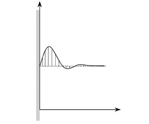
Figure 5 illustrates the modification of the mean flow for two sets of parameters:  ${{Pr}} = 6.7$ for different $\lambda$, and $\lambda = 0$ for different ${{Pr}}$. For ${{Pr}}=6.7$, the position of the maximum value for the modification of the mean flow moves towards the wall at higher gradient ratio $\lambda$ due to a thinner boundary layer. And the maximum value of the correction of velocity and temperature increases with an increase of $\lambda$. However, near the wall, the defect of velocity decreases with an increase of $\lambda$ (figure 5a), which is contrary to the temperature (figure 5b). The modifications of the mean flow with different ${{Pr}}$ for an isothermal wall ( $\lambda =0$) are shown in figure 5( $c$,
$c$, $d$). With an increase of ${{Pr}}$, the amount of correction increases constantly, but the position of the maximum value does not change monotonically. Nevertheless, the curves have a common feature: there is a maximum value and two minimum values. And the value of basic flow near the wall will decrease to some extent.

Figure 5. Modification of the mean flow. ( $a$) Velocity and ( $b$) temperature as functions of $\eta$ for different values of $\lambda$ with ${{Pr}} = 6.7$. ( $c$) Velocity and ( $d$) temperature as functions of $\eta$ for different values of ${{Pr}}$ with $\lambda = 0$. For the case of ${{Pr}} = 0.1$ in (c,d), the dotted lines are magnified by 100 times.
4.2. Second harmonic of the fundamental $(k = 2, n = 2)$

The equation for the second harmonic is derived by substituting  $k=n=2$ into (A1), and we have
 \begin{equation} \boldsymbol{\mathsf{Q}}^{(2,2)}\boldsymbol{\mathsf{X}}^{(2,2)}=\boldsymbol{\mathsf{F}}^{(2,2)}, \end{equation}
where
 $$\begin{gather} \boldsymbol{\mathsf{Q}}^{(2,2)}= \left(\begin{array}{cc} \displaystyle \dfrac{1}{G} \mathscr{L}_{2}^{2}-\mathscr{M}^{(2,2)}\mathscr{L}_{2}+2\mathrm{i}\alpha F_0''' & \displaystyle \dfrac{\alpha}{\sqrt{2}G}\mathscr{D} \\[10pt] \displaystyle 2\sqrt{2}\mathrm{i}H_0'-\dfrac{4\sqrt{2}}{\alpha G}[1+(\lambda-1)H_0]\mathscr{D} & \displaystyle \dfrac{1}{{{Pr}} \,G}\mathscr{L}_{2}-\mathscr{M}^{(2,2)}-\dfrac{4}{G}(\lambda-1)F_0' \end{array} \right), \end{gather}$$
 $$\begin{gather}\boldsymbol{\mathsf{F}}^{(2,2)}=\left(\begin{array}{c} \displaystyle \sqrt{2}\mathrm{i}(\mathscr{D}\phi^{(1,1)}\mathscr{L}_{1}\phi^{(1,1)}-\phi^{(1,1)}\mathscr{L}_{1}\mathscr{D}\phi^{(1,1)})\\[6pt] \displaystyle \sqrt{2}\mathrm{i}(\mathscr{D}\phi^{(1,1)}\varphi^{(1,1)}-\phi^{(1,1)}\mathscr{D}\varphi^{(1,1)})+\dfrac{4\sqrt{2}}{\alpha G}(\lambda-1)\mathscr{D}\phi^{(1,1)}\varphi^{(1,1)} \end{array} \right). \end{gather}$$
Similarly, (4.6) implies that the fundamental mode interacting with itself leads to the generation of the second harmonic. The amplitude profiles of the second harmonic of the fundamental for different  ${{Pr}}$ and $\lambda$ are shown in figure 6. For given ${{Pr}}=6.7$, it can be seen from figures 6( $a$) and 6( $b$) that the velocity curve contains three peaks, but the temperature curve only has one. And with increasing $\lambda$, all of the peaks approach the wall gradually. Compared with the linear critical mode for velocity disturbance in Tao et al. (Reference Tao, LeQuéré and Xin2004b), the position of the second and third peaks of $|\phi _{\eta }^{(2,2)}|$ almost coincides with the extreme position of the linear mode corresponding to the buoyancy-driven instability mode. Besides, the distinction is that there will be an additional peak in the near-wall region for the velocity of the second harmonic of the fundamental, and the emergence of this peak is related to the interaction between linear modes. For $\lambda =0$, the maximum value of each curve increases as ${{Pr}}$ increases (see figure 6c,d). In figure 6( $c$), the amplitude profiles for ${{Pr}}=0.72$ and 6.7 have three peaks, while for a large or small value of ${{Pr}}$, the profiles have only two peaks. Considering the physical meaning of the Prandtl number, the number of peaks in the second harmonic of the fundamental may be related to the competition between momentum transport and heat transport.

Figure 6. Amplitude profiles of the second harmonic of the fundamental. ( $a$) Velocity and ( $b$) temperature as functions of $\eta$ for different values of $\lambda$ with ${{Pr}} = 6.7$. ( $c$) Velocity and ( $d$) temperature as functions of $\eta$ for different values of ${{Pr}}$ with $\lambda = 0$. For the case of ${{Pr}} = 0.1$ in (c,d), the dotted lines are magnified by 100 and 20 times, respectively.
4.3. Landau coefficient $(k = 1, n = 3)$

At  $O(A^{3})$, we derive an equation for the distortion of the fundamental mode $\phi ^{(1,3)}$ and $\varphi ^{(1,3)}$ by substituting $k = 1$ and $n = 3$ into (A1):
 \begin{equation} \boldsymbol{\mathsf{Q}}^{(1,3)}\boldsymbol{\mathsf{X}}^{(1,3)}=(a^{(2)}+\mathrm{i}b^{(2)})\boldsymbol{\mathsf{S}}\boldsymbol{\mathsf{X}}^{(1,1)}+\boldsymbol{\mathsf{F}}^{(1,3)}, \end{equation}
where
 \begin{gather}
\boldsymbol{\mathsf{Q}}^{(1,3)}= \left(
\begin{array}{@{}cc@{}} \displaystyle \dfrac{1}{G}
\mathscr{L}_{1}^{2}-\mathscr{M}^{(1,3)}\mathscr{L}_{1}+\mathrm{i}\alpha
F_0''' & \displaystyle \dfrac{\alpha}{\sqrt{2}G}\mathscr{D}
\\[10pt] \displaystyle
\sqrt{2}\mathrm{i}H_0'-\dfrac{4\sqrt{2}}{\alpha
G}[1+(\lambda-1)H_0]\mathscr{D} & \displaystyle
\dfrac{1}{{{Pr}}
\,G}\mathscr{L}_{1}-\mathscr{M}^{(1,3)}-\dfrac{4}{G}(\lambda-1)F_0'
\end{array} \right), \end{gather}
\begin{gather}
\boldsymbol{\mathsf{Q}}^{(1,3)}= \left(
\begin{array}{@{}cc@{}} \displaystyle \dfrac{1}{G}
\mathscr{L}_{1}^{2}-\mathscr{M}^{(1,3)}\mathscr{L}_{1}+\mathrm{i}\alpha
F_0''' & \displaystyle \dfrac{\alpha}{\sqrt{2}G}\mathscr{D}
\\[10pt] \displaystyle
\sqrt{2}\mathrm{i}H_0'-\dfrac{4\sqrt{2}}{\alpha
G}[1+(\lambda-1)H_0]\mathscr{D} & \displaystyle
\dfrac{1}{{{Pr}}
\,G}\mathscr{L}_{1}-\mathscr{M}^{(1,3)}-\dfrac{4}{G}(\lambda-1)F_0'
\end{array} \right), \end{gather}
and the expression for the inhomogeneous term  $\boldsymbol{\mathsf{F}}^{(1,3)}$ represents the quadratic nonlinear terms that arise from the product of two Fourier series:
 \begin{equation}
\boldsymbol{\mathsf{F}}^{(1,3)}= \left(
\begin{array}{@{}c@{}} \displaystyle \mathscr{N}_{M}^{01} +
\mathscr{N}_{M}^{12}\\ \displaystyle \mathscr{N}_{E}^{01} +
\mathscr{N}_{E}^{10} + \mathscr{N}_{E}^{12} +
\mathscr{N}_{E}^{21}\\ \end{array} \right),
\end{equation}
\begin{equation}
\boldsymbol{\mathsf{F}}^{(1,3)}= \left(
\begin{array}{@{}c@{}} \displaystyle \mathscr{N}_{M}^{01} +
\mathscr{N}_{M}^{12}\\ \displaystyle \mathscr{N}_{E}^{01} +
\mathscr{N}_{E}^{10} + \mathscr{N}_{E}^{12} +
\mathscr{N}_{E}^{21}\\ \end{array} \right),
\end{equation}
with
 \begin{gather} \mathscr{N}_{M}^{01} ={-}\sqrt{2}\mathrm{i}[(\mathscr{D}\phi^{(0,2)}+\mathscr{D}\overline{\phi^{(0,2)}})\mathscr{L}_{1}\phi^{(1,1)}-\phi^{(1,1)}\mathscr{L}_{0}(\mathscr{D}\phi^{(0,2)}+\mathscr{D}\overline{\phi^{(0,2)}})], \end{gather}
 \begin{gather} \mathscr{N}_{M}^{12} ={-}\sqrt{2}\mathrm{i}(2\mathscr{D}\overline{\phi^{(1,1)}}\mathscr{L}_{2}\phi^{(2,2)}-\mathscr{D}\phi^{(2,2)}\mathscr{L}_{1}\overline{\phi^{(1,1)}}\nonumber\\ \hspace{2pc} -2\phi^{(2,2)}\mathscr{L}_{1}\mathscr{D}\overline{\phi^{(1,1)}}+\overline{\phi^{(1,1)}}\mathscr{L}_{2}\mathscr{D}\phi^{(2,2)}), \end{gather}
 $$\begin{gather} \mathscr{N}_{E}^{01} ={-}\sqrt{2}\mathrm{i}(\mathscr{D}\phi^{(0,2)}+\mathscr{D}\overline{\phi^{(0,2)}})\varphi^{(1,1)} -\frac{4\sqrt{2}}{\alpha G}(\lambda-1)(\mathscr{D}\phi^{(0,2)}+\mathscr{D}\overline{\phi^{(0,2)}})\varphi^{(1,1)}, \end{gather}$$
 $$\begin{gather}\mathscr{N}_{E}^{10} = \sqrt{2}\mathrm{i}\phi^{(1,1)}(\mathscr{D}\varphi^{(0,2)}+\mathscr{D}\overline{\varphi^{(0,2)}})-\frac{4\sqrt{2}}{\alpha G}(\lambda-1)\mathscr{D}\phi^{(1,1)}(\varphi^{(0,2)}+\overline{\varphi^{(0,2)}}), \end{gather}$$
 $$\begin{gather}\mathscr{N}_{E}^{12} ={-}\sqrt{2}\mathrm{i}(2\mathscr{D}\overline{\phi^{(1,1)}}\varphi^{(2,2)}+\overline{\phi^{(1,1)}}\mathscr{D}\varphi^{(2,2)}) -\frac{4\sqrt{2}}{\alpha G}(\lambda-1)\mathscr{D}\overline{\phi^{(1,1)}}\varphi^{(2,2)}, \end{gather}$$
 $$\begin{gather}\mathscr{N}_{E}^{21} = \sqrt{2}\mathrm{i}(\mathscr{D}\phi^{(2,2)}\overline{\varphi^{(1,1)}}+2\phi^{(2,2)}\mathscr{D}\overline{\varphi^{(1,1)}})-\frac{4\sqrt{2}}{\alpha G}(\lambda-1)\mathscr{D}\phi^{(2,2)}\overline{\varphi^{(1,1)}}. \end{gather}$$
The subscripts M and E refer to terms that originate from the momentum and energy equations. The superscripts 0, 1 and 2 represent the modification of the mean flow, fundamental mode and second harmonic, respectively. For example, in the energy equation,  $\mathscr {N}_{E}^{01}$ is the interaction of the modification of the mean flow for velocity with the fundamental mode for temperature.
Equation (4.7) is an inhomogeneous differential equation that has a unique solution if and only if a solvability condition or the Fredholm alternative is satisfied. The solvability condition states that the inhomogeneous term has to be orthogonal to the solution of the adjoint homogeneous problem. The homogeneous adjoint problem associated with (4.7) is given as
 \begin{equation} \boldsymbol{\mathsf{Q}}^{(1,3){\dagger}}\boldsymbol{\mathsf{X}}^{(1,3){\dagger}}=0, \end{equation}
where  $\boldsymbol{\mathsf{X}}^{(1,3){\dagger} }=(\phi ^{(1,3){\dagger} },\varphi ^{(1,3){\dagger} })^{\mathrm {T}}$ and the adjoint operator $\boldsymbol{\mathsf{Q}}^{(1,3){\dagger} }$ is defined through the relationship
 \begin{equation} \langle f, \mathscr{L} g\rangle = \langle \mathscr{L}^{{{\dagger}}} f, g\rangle. \end{equation}
Thus,  $\boldsymbol{\mathsf{Q}}^{(1,3){\dagger} }$ can be obtained by integration by parts. Then we obtain
 \begin{equation} \boldsymbol{\mathsf{Q}}^{(1,3){\dagger}}= \displaystyle \left(\begin{array}{@{}cc@{}} \displaystyle \dfrac{1}{G} \mathscr{L}_{1}^{2}-\overline{\mathscr{M}^{(1,3)}}\mathscr{L}_{1} & \displaystyle -\sqrt{2}\mathrm{i}H_0'+\dfrac{4\sqrt{2}}{\alpha G}[\mathscr{D}+(\lambda-1)(H_0\mathscr{D}+H_0')] \\ \quad +2\mathrm{i}\alpha F_0'' \mathscr{D} & {}\\[8pt] \displaystyle -\dfrac{\alpha}{\sqrt{2}G}\mathscr{D} & \displaystyle \dfrac{1}{{{Pr}} \,G}\mathscr{L}_{1}-\overline{\mathscr{M}^{(1,3)}}-\dfrac{4}{G}(\lambda-1)F_0' \end{array} \right), \end{equation}
with the adjoint boundary conditions
 \begin{equation} \phi^{(1,3){\dagger}}(0) = \mathscr{D}\phi^{(1,3){\dagger}}(0) = \mathscr{D}\phi^{(1,3){\dagger}}(\infty) = \varphi^{(1,3){\dagger}}(0) = \varphi^{(1,3){\dagger}}(\infty) = 0. \end{equation}
The amplitude of the adjoint solution is normalized by
 \begin{equation} \langle
\phi^{(1,3){\dagger}}, \phi^{(1,3){\dagger}} \rangle +
\langle \varphi^{(1,3){\dagger}},
\varphi^{(1,3){\dagger}} \rangle = 1.
\end{equation}
\begin{equation} \langle
\phi^{(1,3){\dagger}}, \phi^{(1,3){\dagger}} \rangle +
\langle \varphi^{(1,3){\dagger}},
\varphi^{(1,3){\dagger}} \rangle = 1.
\end{equation}
The adjoint solutions  $\phi ^{(1,3){\dagger} }$ and $\varphi ^{(1,3){\dagger} }$ for ${{Pr}}=6.7$ with different $\lambda$ are displayed in figure 10 in Appendix B. The Fredholm alternative for the present case means that the right-hand side of (4.7) has to be orthogonal to the solution of the adjoint problem (4.11). The Landau coefficient is then obtained:
 \begin{equation} a^{(2)}+\mathrm{i}b^{(2)}={-}\frac{\left \langle \boldsymbol{\mathsf{X}}^{(1,3){\dagger}}, \boldsymbol{\mathsf{F}}^{(1,3)} \right \rangle}{\left \langle \boldsymbol{\mathsf{X}}^{(1,3){\dagger}}, \boldsymbol{\mathsf{S}}\boldsymbol{\mathsf{X}}^{(1,1)} \right \rangle} = \sigma_{M}^{01} + \sigma_{M}^{12} + \sigma_{E}^{01} + \sigma_{E}^{10} + \sigma_{E}^{12} + \sigma_{E}^{21}, \end{equation}
with
 $$\begin{gather} \sigma_{M}^{01} = {-}\frac{\left \langle {\phi}^{(1,3){\dagger}}, \mathscr{N}_{M}^{01} \right \rangle} {\left \langle \boldsymbol{\mathsf{X}}^{(1,3){\dagger}}, \boldsymbol{\mathsf{S}}\boldsymbol{\mathsf{X}}^{(1,1)} \right \rangle}, \quad \sigma_{M}^{12} ={-}\frac{\left \langle {\phi}^{(1,3){\dagger}}, \mathscr{N}_{M}^{12} \right \rangle} {\left \langle \boldsymbol{\mathsf{X}}^{(1,3){\dagger}}, \boldsymbol{\mathsf{S}}\boldsymbol{\mathsf{X}}^{(1,1)} \right \rangle}, \end{gather}$$
 $$\begin{gather}\sigma_{E}^{01} ={-}\frac{\left \langle {\varphi}^{(1,3){\dagger}}, \mathscr{N}_{E}^{01} \right \rangle} {\left \langle \boldsymbol{\mathsf{X}}^{(1,3){\dagger}}, \boldsymbol{\mathsf{S}}\boldsymbol{\mathsf{X}}^{(1,1)} \right \rangle}, \quad \sigma_{E}^{10} ={-}\frac{\left \langle {\varphi}^{(1,3){\dagger}}, \mathscr{N}_{E}^{10} \right \rangle} {\left \langle \boldsymbol{\mathsf{X}}^{(1,3){\dagger}}, \boldsymbol{\mathsf{S}}\boldsymbol{\mathsf{X}}^{(1,1)} \right \rangle}, \end{gather}$$
 $$\begin{gather}\sigma_{E}^{12} ={-}\frac{\left \langle {\varphi}^{(1,3){\dagger}}, \mathscr{N}_{E}^{12} \right \rangle} {\left \langle \boldsymbol{\mathsf{X}}^{(1,3){\dagger}}, \boldsymbol{\mathsf{S}}\boldsymbol{\mathsf{X}}^{(1,1)} \right \rangle}, \quad \sigma_{E}^{21} ={-}\frac{\left \langle {\varphi}^{(1,3){\dagger}}, \mathscr{N}_{E}^{21} \right \rangle} {\left \langle \boldsymbol{\mathsf{X}}^{(1,3){\dagger}}, \boldsymbol{\mathsf{S}}\boldsymbol{\mathsf{X}}^{(1,1)} \right \rangle}, \end{gather}$$
where  $\sigma _{M}^{01}$ is the feedback of the mean flow distortion on the fundamental mode, $\sigma _{E}^{12}$ is the feedback of the second harmonic on the fundamental mode, etc. The supercritical and subcritical types of instability (bifurcation) are identified by the sign of $a^{(2)}$. For $a^{(0)} > 0$ and $a^{(2)} < 0$, a finite-amplitude equilibrium solution can be achieved after the infinitesimal state has become unstable, which is known as supercritical bifurcation. For $a^{(0)} < 0$ and $a^{(2)} > 0$, a finite-amplitude equilibrium solution can be achieved before the base state has become linearly unstable, which is known as subcritical bifurcation.
Utilizing the numerical values in table 2,  $a^{(2)}$ and $b^{(2)}$ are computed over a range of critical parameters. Several tests are performed for different computational domains $\eta _{{max}}$ and Chebyshev points $N$ to ensure numerical convergence, and the results are shown in table 4 in Appendix C. The result of the Landau coefficient $a^{(2)}$ from (4.16) for different ${{Pr}}$ and $\lambda$ at the least unstable parameter is shown in figure 7(a). For the isothermal ( $\lambda = 0$) and uniform-heat-flux ( $\lambda = 1$) walls, we found that $a^{(2)} < 0$ for all the cases ( $10^{-1} \leqslant {{Pr}} \leqslant 10^{4}$) considered here, which means the flow is supercritical instability. However, with an increase in the temperature gradient ratio, $a^{(2)} > 0$ is obtained for a large value of ${{Pr}}$ and this corresponds to the subcritical solution. The results are therefore limited to ${{Pr}} \leqslant 10^{4}$.

Figure 7. ( $a$) Variation of the Landau coefficient $a^{(2)}$ with ${{Pr}}$ for different $\lambda$. The lines are obtained by spline interpolation. ( $b$) Phase diagram in the ( ${{Pr}}, \lambda$) plane. The grey thick solid line indicates the boundary $a^{(2)}=0$ separating the supercritical region (below) and subcritical region (above).
The boundary  $a^{(2)} = 0$ is shown in figure 7( $b$), which separates the ( ${{Pr}}, \lambda$) plane into a supercritical region (below) and subcritical region (above). It can be seen that, for $0 \leqslant \lambda < 2$, only a supercritical bifurcation exists when ${{Pr}} \leqslant 2800$. Moreover, with an increase of temperature gradient ratio, the corresponding value of ${{Pr}}$ at the boundary gradually decreases. It is illustrated in figure 7( $b$) that subcritical bifurcations are observed only for large temperature gradient ratios and Prandtl numbers. Close examination for basic flow $F_0'(\eta )$ and $H_0(\eta )$ reveals that for higher temperature gradient ratio and Prandtl number, the position of the maximum amplitude of velocity moves towards the wall and the temperature gradients near the wall increase due to a thinner boundary layer. And the absolute values of the maximum and the minimum streamwise velocities also decrease with an increase of ${{Pr}}$ and $\lambda$. These characteristics of basic flow may be related to the fact of the existence of subcritical bifurcation at high ${{Pr}}$ and $\lambda$. It is worth mentioning that the parameter values from Iyer & Kelly (Reference Iyer and Kelly1978) all lie within the region where the bifurcation is supercritical, which is consistent with their results. Besides, the parameter values for the discussion on the convective and absolute instabilities from Krizhevsky et al. (Reference Krizhevsky, Cohen and Tanny1996) and Tao et al. (Reference Tao, LeQuéré and Xin2004b) are also shown in figure 7( $b$). The bifurcation types corresponding to these parameters are still supercritical. In fact, the above results suggest that most common fluids, such as air ( ${{Pr}}=0.72$), water ( ${{Pr}}=6.7$) and argon ( ${{Pr}}=23$), are below the boundary and belong to supercritical bifurcation. For fluids such as glycerine ( ${{Pr}} \approx 2000$), the buoyancy layer can experience a subcritical bifurcation under a larger temperature gradient ratio.
4.4. Threshold amplitude
In this subsection, we discuss the nature of bifurcation for the appearance of finite-amplitude nonlinear equilibrium solutions. We rewrite the Landau equation (2.13a,b) as
 \begin{equation} \frac{\mathrm{d} A}{\mathrm{d} \tau} = A a^{(0)} + A^{3}a^{(2)} + A^{5}a^{(4)} + \cdots . \end{equation}
This series is also known as the Stuart–Landau series (Stuart Reference Stuart1960; Watson Reference Watson1960), in which  $a^{(0)}$ is the growth rate from linear theory and the Landau coefficients $a^{(2)}, a^{(4)},\ldots$ are nonlinear corrections to the linear growth rate as mentioned above. Only the leading-order term of the Landau coefficient is of concern here and the stationary equilibrium amplitude solution $A_e$ for (4.18) has two possible solutions. If $a^{(0)}$ and $a^{(2)}$ are of the same sign, only the zero-amplitude state exists as an equilibrium solution. If $a^{(0)}$ and $a^{(2)}$ are of opposite sign, as time increases, we have a steady state:
 \begin{equation} A_e = \sqrt{-\frac{a^{(0)}}{a^{(2)}}}. \end{equation}
Figure 8 plots the equilibrium amplitude  $A_e$ in the neighbourhood of the critical instability $\epsilon = (G-G_c)/G_c \ll 1$ for different values of $\lambda$ and ${{Pr}}$ when the instabilities are supercritical. The equilibrium amplitude increases smoothly with an increase of $\epsilon$, and we have $A_e \sim \epsilon ^{-1/2}$ according to the Taylor expansion. For given $\lambda$ and ${{Pr}}$, the threshold amplitude will reach a stable nonlinear state, which limits the basin of attraction of the laminar flow. When $\lambda =0$, the equilibrium amplitude decreases with an increase of ${{Pr}}$ (see figure 8a), i.e. the flow becomes more sensitive to small perturbations. Figure 8( $b$) illustrates that $A_e$ decreases significantly as the temperature gradient ratio increases. Apparently, the magnitude of $A_e$ for the flow near an isothermal wall is twice that for a uniform-heat-flux wall.

Figure 8. Variation of equilibrium amplitude as a function of  $\epsilon = (G-G_c)/G_c$ for ( $a$)
$a$)  $\lambda =0$ with different ${{Pr}}$ and ( $b$)
$b$)  ${{Pr}}=6.7$ with different $\lambda$. The bifurcation is supercritical in each case.
Figure 9 shows a series of bifurcation diagrams for six values of  ${{Pr}}$ at $\lambda =5$. It can be seen that, with increasing ${{Pr}}$, the equilibrium amplitude increases gradually when the flow works in the linearly unstable regime $\epsilon > 0$. The instability here is of supercritical type, which is indicated by solid lines in figure 9. However, when the value of ${{Pr}}$ continues to increase, the bifurcation type becomes subcritical immediately (dashed lines) and the value of $A_e$ decreases. It is noteworthy that the buoyancy flow is nonlinearly stable for $A < A_e$ and unstable for $A > A_e$, and the finite-amplitude unstable branch in figure 9 provides a threshold for nonlinear stability. It is obtained that the critical Prandtl number at which this switchover between the subcritical and supercritical bifurcations occurs is ${{Pr}} \approx 285$.

Figure 9. Variation of equilibrium amplitude as a function of  $\epsilon = (G-G_c)/G_c$ for $\lambda =5$ with different ${{Pr}}$. The bifurcation type changes from supercritical (solid lines) to subcritical (dashed lines).
In order to analyse the nonlinear effects that control the type of bifurcation, the contributions of the different terms  $\sigma _{M}^{01}, \sigma _{M}^{12},\ldots$ in (4.16) that affect the value of $a^{(2)}$ are given in table 3 for the parameters analysed in figure 9. There are several points worth noting. First, the fundamental modes $\phi ^{(1,1)}$ in the momentum equation play a minor role in these effects since the corresponding contributions $\sigma _{M}^{01}$ and $\sigma _{M}^{12}$ are of small magnitude in comparison with the contributions associated with that in the energy equation. A second important point is that the values of $\sigma _{E}^{10}$ and $\sigma _{E}^{12}$ are always negative, which means the interaction between the fundamental mode for velocity and temperature is beneficial to supercritical bifurcation. A last important point revealed in table 3 is that the buoyancy-driven effects are crucial since for different ${{Pr}}$, the values of $\sigma _{E}^{01} + \sigma _{E}^{21}$ are greater than zero. The flow energy from distortion of the mean flow $\phi ^{(0,2)}$ to the fundamental $\varphi ^{(1,1)}$ is described by $\sigma _{E}^{01}$, while $\sigma _{E}^{21}$ represents the flow energy from the fundamental $\varphi ^{(1,1)}$ to the second harmonic $\phi ^{(2,2)}$. This suggests that the interaction of the modification of the mean flow and second harmonic for velocity with the fundamental mode for temperature plays an important role in the subcritical bifurcation. Considering that the buoyancy-driven instability becomes increasingly important as the Prandtl number is increased (Gill & Davey Reference Gill and Davey1969), the coupling between the energy equation and the Orr–Sommerfeld equation may provide some clues for revealing the mechanism of changing bifurcation.
Table 3. Landau coefficient and real part of the contribution of the nonlinear terms for different Prandtl number  ${{Pr}}$ at temperature gradient ratio $\lambda =5$.

5. Conclusion
In this work, we have studied the finite-amplitude instability of the natural convection flow on a vertically heated plate, where the ambient fluid and the wall have independent temperature gradients. As mentioned in the introduction, the linear stability was investigated by Tao et al. (Reference Tao, LeQuéré and Xin2004b), and the finite-amplitude solution (Iyer & Kelly Reference Iyer and Kelly1978) arising from the critical instability was studied only for a uniform-heat-flux surface ( $\lambda =1$). Only supercritical bifurcation was found in their analysis. In order to extend their results, a weakly nonlinear theory is developed to describe the nonlinear instability of the buoyancy-driven boundary layer. The amplitude expansion method of Reynolds & Potter (Reference Reynolds and Potter1967) is adapted to the present nonlinear problem. At different orders, the nonlinear stability problem is reduced to a sequence of linear inhomogeneous differential equations. Then, the basic flow, the fundamental mode, the related modification of the base flow, the second harmonics and Landau coefficients are obtained.
The flow is governed by three parameters: modified Grashof number  $G$, Prandtl number ${{Pr}}$ and temperature gradient ratio $\lambda$. The present parametric study is mainly focused on the critical mode of the linear problem, except in the discussion on equilibrium amplitude. The main conclusions of the analysis are as follows. For the distortion of mean flow, the maximum value of the correction amount of velocity and temperature increases with an increase of $\lambda$ for fixed ${{Pr}}=6.7$. With an increase of ${{Pr}}$, the maximum value of the distortion of mean flow increases constantly for the isothermal surface. For the second harmonic generated by the fundamental mode interacting with itself, when ${{Pr}}=6.7$, the position of the second and third peaks of velocity almost coincides with the extreme position of the linear mode corresponding to the buoyancy-driven instability mode. And the modulus of the harmonic increases with increasing $\lambda$. The Landau coefficients are determined from the solvability condition (the Fredholm alternative) at $O(A^{3})$. We have identified the boundary for Landau coefficient $a^{(2)}=0$. For Prandtl number above the critical value, the bifurcation is subcritical. Otherwise, it is a supercritical bifurcation. It is shown that, for $0 \leqslant \lambda < 2$, only supercritical bifurcation exists when ${{Pr}} \leqslant 2800$. The current result is consistent with that of Iyer & Kelly (Reference Iyer and Kelly1978). In addition, the threshold amplitude of the bifurcation is determined as well. The threshold amplitude decreases with increasing ${{Pr}}$ for the isothermal wall. For ${{Pr}}=6.7$, the threshold amplitude also decreases with increasing $\lambda$. By analysing the contribution of the nonlinear terms in the Landau coefficient for the bifurcation type changing from supercritical to subcritical, it is revealed that the interaction of the modification of the mean flow and second harmonic for velocity with the fundamental mode for temperature plays an important role in subcritical bifurcation.
Although only two-dimensional disturbances are considered in this paper, the present configuration can be extended to analyse the finite-amplitude instability in the three-dimensional buoyancy layer. We have only calculated the first Landau coefficient at cubic order in  $A$. For subcritical bifurcations and significant deviation from the critical parameter, the higher-order Landau coefficients are needed to identify the stable finite-amplitude solution. Despite this, we anticipate that the results provided in this paper may serve as a guide for the sequence of bifurcation leading to turbulence for such a buoyancy-driven flow system. We emphasize that the experimental data in the literature are very scarce. This is also very convenient and helpful in the experimental study of near-onset dynamics, in particular, for high-Prandtl-number fluids for which the bifurcation should be subcritical. This will be the subject of future exploration.
Funding
This work was supported by the National Natural Science Foundation of China (no. 12072177).
Declaration of interests
The authors have no conflicts to disclose.
Appendix A. The equations for $\phi ^{(k,n)}(\eta )$ and $\varphi ^{(k,n)}(\eta )$


The ordinary differential equations for  $\phi ^{(k,n)}(\eta )$ and $\varphi ^{(k,n)}(\eta )$ are as follows:
 \begin{gather} \underbrace{\frac{\mathrm{d} A}{\mathrm{d} t}\frac{\partial \zeta}{\partial A}}_{T_1}+\underbrace{\left[\omega+\frac{\mathrm{d} \omega}{\mathrm{d} A}\left(t\frac{\mathrm{d} A}{\mathrm{d} t}\right)\right]\frac{\partial \zeta}{\partial \theta}}_{T_2}+\underbrace{\frac{\partial\psi}{\partial \eta}\frac{\partial \zeta}{\partial \theta}}_{N_1}-\underbrace{\frac{\partial\psi}{\partial \theta}\frac{\partial \zeta}{\partial \eta}}_{N_2}=\underbrace{\frac{1}{G}\boldsymbol{\nabla}_{\alpha}^{2} \zeta}_{D_1}+\underbrace{\frac{\alpha}{\sqrt{2}G}\frac{\partial T}{\partial \eta}}_{R_1}, \end{gather}
 \begin{gather} \underbrace{\frac{\mathrm{d} A}{\mathrm{d} t}\frac{\partial T}{\partial A}}_{T_3}+\underbrace{\left[\omega+\frac{\mathrm{d} \omega}{\mathrm{d} A}\left(t\frac{\mathrm{d} A}{\mathrm{d} t}\right)\right]\frac{\partial T}{\partial \theta}}_{T_4}+\underbrace{\frac{\partial\psi}{\partial \eta}\frac{\partial T}{\partial \theta}}_{N_3}-\underbrace{\frac{\partial\psi}{\partial \theta}\frac{\partial T}{\partial \eta}}_{N_4}\nonumber\\ \hspace{10pt}= \underbrace{\frac{1}{{{Pr}} \,G}\boldsymbol{\nabla}_{\alpha}^{2}T}_{D_2} -\underbrace{\frac{4\sqrt{2}\varepsilon [1+(\lambda-1)T]}{\alpha f}\frac{\partial\psi}{\partial \eta}}_{R_2}+ O(\varepsilon^{2}), \end{gather}
where the additional terms at  $O(\varepsilon ^{2})$ are ignored. We separate each term of (A1) with
 \begin{gather} T_1=2\alpha^{2}\frac{f_{\theta}}{f}\mathrm{i}k\sum_{q=k}^{n}qa^{(n-q)}\phi^{(k,q)}+\sum_{q=k}^{n}qa^{(n-q)}\mathscr{L}_{k}\phi^{(k,q)}, \end{gather}
 \begin{gather} T_2=\frac{f_{\theta}}{f}\sum_{q=k}^{n}b^{(n-q)}(\mathscr{L}_{k}-2k^{2}\alpha^{2})\phi^{(k,q)}+\mathrm{i}k\sum_{q=k}^{n}b^{(n-q)}\mathscr{L}_{k}\phi^{(k,q)}, \end{gather}
 \begin{align} N_1&=\sqrt{2}\left\{\sum_{j=0}^{k}\sum_{q=j}^{n-k+j}\mathscr{D}\phi^{(k-j,n-q)}\mathrm{i}j\mathscr{L}_{j}\phi^{(j,q)}\right.\nonumber\\ &\quad +\frac{1}{1+\delta_{k0}}\left[\sum_{j=0}^{\infty}\sum_{q=k+j}^{n-j}\mathscr{D} \overline{\phi^{(j,n-q)}}\mathrm{i}(k+j)\mathscr{L}_{k+j}\phi^{(k+j,q)}\right.\nonumber\\ &\quad \left. \left.-\sum_{j=0}^{\infty}\sum_{q=j}^{n-k-j}\mathscr{D}\phi^{(k+j,n-q)}\mathrm{i}j\mathscr{L}_{j} \overline{\phi^{(j,q)}}\right]\right\}\nonumber\\ &\quad +\sqrt{2}\frac{f_{\theta}}{f}\left\{\sum_{j=0}^{k}\sum_{q=j}^{n-k+j} \mathscr{D}\phi^{(k-j,n-q)}(\mathscr{L}_{j}-2j^{2}\alpha^{2})\phi^{(j,q)}\right.\nonumber\\ &\quad+\left.\frac{1}{1+\delta_{k0}}\left[\sum_{j=0}^{\infty}\sum_{q=k+j}^{n-j}\mathscr{D} \overline{\phi^{(j,n-q)}}(\mathscr{L}_{k+j}-2(k+j)^{2}\alpha^{2})\phi^{(k+j,q)}\right.\right.\nonumber\\ \displaystyle &\quad\left.\left.+\sum_{j=0}^{\infty}\sum_{q=j}^{n-k-j}\mathscr{D}\phi^{(k+j,n-q)}(\mathscr{L}_{j}-2j^{2}\alpha^{2})\overline{\phi^{(j,q)}}\right]\right\}, \end{align}
 \begin{align} N_2&=\sqrt{2}\left\{\sum_{j=0}^{k}\sum_{q=j}^{n-k+j}\mathrm{i}(k-j)\phi^{(k-j,n-q)}\mathscr{L}_{j}\mathscr{D}\phi^{(j,q)}\right.\nonumber\\ &\quad+\frac{1}{1+\delta_{k0}}\left[\sum_{j=0}^{\infty}\sum_{q=j}^{n-k-j}\mathrm{i}(k+j)\phi^{(k+j,n-q)} \mathscr{L}_{j}\mathscr{D}\overline{\phi^{(j,q)}}\right. \nonumber\\ &\quad \left.\left. -\sum_{j=0}^{\infty}\sum_{q=k+j}^{n-j}\mathrm{i}j\overline{\phi^{(j,n-q)}}\mathscr{L}_{k+j}\mathscr{D}\phi^{(k+j,q)}\right]\right\}\nonumber\\ &\quad +\sqrt{2}\frac{f_{\theta}}{f}\left[\sum_{j=0}^{k}\sum_{q=j}^{n-k+j}\phi^{(k-j,n-q)}\mathscr{L}_{j}\mathscr{D}\phi^{(j,q)}\right. \nonumber\\ &\quad+\frac{1}{1+\delta_{k0}}\left(\sum_{j=0}^{\infty}\sum_{q=k+j}^{n-j}\overline{\phi^{(j,n-q)}} \mathscr{L}_{k+j}\mathscr{D}\phi^{(k+j,q)}\right.\nonumber\\ &\quad \left.\left.+\sum_{j=0}^{\infty}\sum_{q=j}^{n-k-j}\phi^{(k+j,n-q)}\mathscr{L}_{j}\mathscr{D} \overline{\phi^{(j,q)}}\right)\right] \nonumber\\ &\quad +2\sqrt{2}\alpha^{2}\frac{f_{\theta}}{f}\left\{-\sum_{j=0}^{k}\sum_{q=j}^{n-k+j}(k-j)j\phi^{(k-j,n-q)}\mathscr{D}\phi^{(j,q)}\right.\nonumber\\ &\quad+\frac{1}{1+\delta_{k0}}\left[\sum_{j=0}^{\infty}\sum_{q=k+j}^{n-j}j(k+j)\overline{\phi^{(j,n-q)}} \mathscr{D}\phi^{(k+j,q)}\right.\nonumber\\ &\quad \left.\left.+\sum_{j=0}^{\infty}\sum_{q=j}^{n-k-j}(k+j)j\phi^{(k+j,n-q)} \mathscr{D}\overline{\phi^{(j,q)}}\right]\right\}, \end{align}
 \begin{gather} D_1=\frac{1}{G}\left(4\alpha^{2}\frac{f_{\theta}}{f}\mathrm{i}k\mathscr{L}_{k}\phi^{(k,n)}+\mathscr{L}_{k}^{2}\phi^{(k,n)}\right), \quad R_1=\frac{\alpha}{\sqrt{2}G}\mathscr{D}\varphi^{(k,n)}, \end{gather}
 \begin{gather} T_3=\sum_{q=k}^{n}qa^{(n-q)}\varphi^{(k,q)}, \quad T_4=\mathrm{i}k\sum_{q=k}^{n}b^{(n-q)}\varphi^{(k,q)}, \quad D_2=\frac{1}{{{Pr}}\,G}\mathscr{L}_{k}\varphi^{(k,n)}, \end{gather}
 \begin{align}
N_3&=\sqrt{2}\left\{\sum_{j=0}^{k}\sum_{q=j}^{n-k+j}\mathscr{D}\phi^{(k-j,n-q)}\mathrm{i}j\varphi^{(j,q)}\right.\nonumber\\
&\quad\left.+\frac{1}{1+\delta_{k0}}\left[\sum_{j=0}^{\infty}\sum_{q=k+j}^{n-j}\mathscr{D}\overline{\phi^{(j,n-q)}}\mathrm{i}(k+j)\varphi^{(k+j,q)}\,{-}\sum_{j=0}^{\infty}\sum_{q=j}^{n-k-j}\mathscr{D}\phi^{(k+j,n-q)}\mathrm{i}j\overline{\varphi^{(j,q)}}\!\right]\!\right\}\!,
\end{align}
\begin{align}
N_3&=\sqrt{2}\left\{\sum_{j=0}^{k}\sum_{q=j}^{n-k+j}\mathscr{D}\phi^{(k-j,n-q)}\mathrm{i}j\varphi^{(j,q)}\right.\nonumber\\
&\quad\left.+\frac{1}{1+\delta_{k0}}\left[\sum_{j=0}^{\infty}\sum_{q=k+j}^{n-j}\mathscr{D}\overline{\phi^{(j,n-q)}}\mathrm{i}(k+j)\varphi^{(k+j,q)}\,{-}\sum_{j=0}^{\infty}\sum_{q=j}^{n-k-j}\mathscr{D}\phi^{(k+j,n-q)}\mathrm{i}j\overline{\varphi^{(j,q)}}\!\right]\!\right\}\!,
\end{align}
 \begin{align} N_4&=\sqrt{2}\left\{\sum_{j=0}^{k}\sum_{q=j}^{n-k+j}{\rm i}(k-j)\phi^{(k-j,n-q)}\mathscr{D}\varphi^{(j,q)}\right.\nonumber\\ &\quad\left.+\frac{1}{1+\delta_{k0}}\left[\sum_{j=0}^{\infty}\sum_{q=j}^{n-k-j}\mathrm{i}(k+j)\phi^{(k+j,n-q)}\mathscr{D}\overline{\varphi^{(j,q)}}-\sum_{j=0}^{\infty}\sum_{q=k+j}^{n-j}\mathrm{i}j\overline{\phi^{(j,n-q)}}\mathscr{D}\varphi^{(k+j,q)}\right]\right\} \nonumber\\ &\quad +\sqrt{2}\frac{f_{\theta}}{f}\left[\sum_{j=0}^{k}\sum_{q=j}^{n-k+j}\phi^{(k-j,n-q)}\mathscr{D}\varphi^{(j,q)}\right. \nonumber\\ &\quad\left.+\frac{1}{1+\delta_{k0}}\left(\sum_{j=0}^{\infty}\sum_{q=k+j}^{n-j}\overline{\phi^{(j,n-q)}}\mathscr{D}\varphi^{(k+j,q)}+\sum_{j=0}^{\infty}\sum_{q=j}^{n-k-j}\phi^{(k+j,n-q)}\mathscr{D}\overline{\varphi^{(j,q)}}\right)\right], \end{align}
 \begin{align} R_2&=\frac{4\sqrt{2}\varepsilon}{\alpha f}\left\{\mathscr{D}\phi^{(k,n)}+(\lambda-1)\left[\sum_{j=0}^{k}\sum_{q=j}^{n-k+j}\varphi^{(k-j,n-q)}D\phi^{(j,q)}\right.\right.\nonumber\\ &\quad\left.\left.+\frac{1}{1+\delta_{k0}}\left(\sum_{j=0}^{\infty}\sum_{q=k+j}^{n-j}\overline{\varphi^{(j,n-q)}}\mathscr{D}\phi^{(k+j,q)}+\sum_{j=0}^{\infty}\sum_{q=j}^{n-k-j}\varphi^{(k+j,n-q)}\mathscr{D}\overline{\phi^{(j,q)}}\right)\right]\right\}, \end{align}
where  $\mathscr {L}_{k}=\mathscr {D}^{2}-k^{2}\alpha ^{2}$, $\mathscr {D}=\mathrm {d}/\mathrm {d}\eta$ and $\delta _{kj} = 0$ if $k \neq j$, $\delta _{kj} = 1$ if $k = j$. The overbar denotes complex conjugation. The factor $1/(1+\delta _{k0})$ in the above equations arises from the product of two Fourier series in which the zeroth-order terms are multiplied by a factor of 2. The corresponding boundary conditions for $k, n \geqslant 1$ are
 \begin{equation} \phi^{(k,n)}(0) = \mathscr{D}\phi^{(k,n)}(0) = \mathscr{D}\phi^{(k,n)}(\infty) = \varphi^{(k,n)}(0) = \varphi^{(k,n)}(\infty) = 0. \end{equation}
Appendix B. Adjoint eigenfunctions for $\phi ^{(1,3){\dagger} }$ and $\varphi ^{(1,3){\dagger} }$


The eigenfunctions of the adjoint linear operator  $\boldsymbol{\mathsf{Q}}^{(1,3){\dagger} }$ in (4.13) for ${{Pr}}=6.7$ with different temperature gradient are shown in figure 10.

Figure 10. Adjoint eigenfunctions for  ${{Pr}}=6.7$. ( $a$) Real and ( $b$) imaginary parts of $\phi ^{(1,3){\dagger} }$. ( $c$) Real and ( $d$) imaginary parts of $\varphi ^{(1,3){\dagger} }$.
Appendix C. Numerical convergence tests
Table 4 shows the results of numerical convergence tests for different computational domains  $\eta _{{max}}$ and Chebyshev points $N$.
$N$.
Table 4. Numerical values of  $a^{(0)}$, $b^{(0)}$, $a^{(2)}$ and $b^{(2)}$ for critical instabilities at different computational domains $\eta _{{max}}$ and Chebyshev points $N$ for two sets of typical parameters. The number of Chebyshev points $N=200$ is used in calculations, which is marked in bold.


