


1. Introduction
Rogue waves are unusually large waves whose wave heights or crest heights are much larger than their surroundings. Haver (Reference Haver2000) suggested as criteria for a rogue wave event within a 20 minute time series of ocean surface waves that the crest height is larger than five quarters of the significant wave height,  $\eta _{max}>1.25H_s$, or the wave height is larger than twice the significant wave height, $H>2H_s$. One physical mechanism that can produce rogue waves is spatial focusing, see Dysthe, Krogstad & Müller (Reference Dysthe, Krogstad and Müller2008). As waves propagate into shallower water, the presence of bottom topography affects the waves through shoaling and refraction. Refraction of waves can lead to spatial focusing of wave energy and, thus, enhance nonlinearity that may provoke non-Gaussian statistics. Rogue waves can occur not only in surface elevation, but also in other quantities such as the velocity field.
The deviation from Gaussian statistics provoked by a sloping bottom was found in field observations before it was measured in the laboratory. In her pioneering work, Bitner (Reference Bitner1980) reported a field experiment of waves propagating into shallower water. Similar field experiments were later reported by Cherneva et al. (Reference Cherneva, Petrova, Andreeva and Guedes Soares2005) and Teutsch et al. (Reference Teutsch, Weisse, Moeller and Krueger2020). From a field data set in the southern North Sea, Teutsch et al. (Reference Teutsch, Weisse, Moeller and Krueger2020) found that there was one buoy that captured more rogue waves than expected and it was located at a rather shallow water depth. Noticeable deviation from Gaussian statistics was found.
Laboratory work not considering statistics include the experiments of waves propagating over a submerged bar of Grue (Reference Grue1992) and Beji & Battjes (Reference Beji and Battjes1993) who showed the growth of bound harmonics triggered by bottom topography. The experiment of Whalin (Reference Whalin1971) considered harmonic wave propagating over a sloping bottom with parallel semicircular contours symmetric in the centre to study the nonlinear effects from the bottom combined with wave refraction. The experiment of Berkhoff, Booij & Radder (Reference Berkhoff, Booij and Radder1982) had an elliptical shoal on the sloping bottom and the waves propagated with an angle. All of the wave tank experiments mentioned previously are widely used as benchmark tests for the validation of deterministic wave models.
Large values for skewness and kurtosis in finite and shallow water depth were observed initially in the laboratory experiment of long-crested irregular waves propagating over a sloping bottom reported by Trulsen, Zeng & Gramstad (Reference Trulsen, Zeng and Gramstad2012). As the waves propagate over a slope, there is a local maximum in the skewness and kurtosis of the surface elevation near the edge of the shallower side of the slope. This behaviour was also demonstrated in numerical simulations by Sergeeva, Pelinovsky & Talipova (Reference Sergeeva, Pelinovsky and Talipova2011), Gramstad et al. (Reference Gramstad, Zeng, Trulsen and Pedersen2013), Viotti & Dias (Reference Viotti and Dias2014), Majda, Moore & Qi (Reference Majda, Moore and Qi2019), Zhang et al. (Reference Zhang, Benoit, Kimmoun, Chabchoub and Hsu2019), Zheng et al. (Reference Zheng, Lin, Li, Adcock, Li and van den Bremer2020), Li et al. (Reference Li, Zheng, Lin, Adcock and van den Bremer2021c) and Lawrence, Trulsen & Gramstad (Reference Lawrence, Trulsen and Gramstad2021b) and in experiments as reported by Kashima, Hirayama & Mori (Reference Kashima, Hirayama and Mori2014), Ma, Dong & Ma (Reference Ma, Dong and Ma2014), Bolles, Speer & Moore (Reference Bolles, Speer and Moore2019), Zhang et al. (Reference Zhang, Benoit, Kimmoun, Chabchoub and Hsu2019), Wang et al. (Reference Wang, Ludu, Zong, Zou and Pei2020), Moore et al. (Reference Moore, Bolles, Majda and Qi2020) and Li et al. (Reference Li, Draycott, Adcock and van den Bremer2021a). Curiously, in a deeper regime with milder slope, Zeng & Trulsen (Reference Zeng and Trulsen2012) did not find this behaviour. Subsequently, Lawrence et al. (Reference Lawrence, Trulsen and Gramstad2021b) confirmed the results by Zeng & Trulsen (Reference Zeng and Trulsen2012) with a more accurate simulation model.
In the work of Janssen, Herbers & Battjes (Reference Janssen, Herbers and Battjes2008) and Janssen & Herbers (Reference Janssen and Herbers2009), they included refraction effect from the bottom topography to study the wave statistics with a frequency-angular spectrum model by Janssen, Herbers & Battjes (Reference Janssen, Herbers and Battjes2006). For directional waves, but without refraction, Ducrozet & Gouin (Reference Ducrozet and Gouin2017) suggested the extreme wave activity is reduced.
A theoretical explanation was developed by Majda et al. (Reference Majda, Moore and Qi2019) based on statistical mechanics of the Korteweg–de Vries (KdV) system. They recognized that the most likely states minimise the Hamiltonian, which in deeper water is associated with minimising the variance of the surface slope, but in shallower water is associated with an increase in the surface displacement skewness, giving rise to the non-Gaussian statistics observed in a number of studies. Another explanation developed by Li et al. (Reference Li, Draycott, Zheng, Lin, Adcock and van den Bremer2021b) suggested the anomalies arise from interaction between linear free and second-order bound waves and new second-order free waves generated due to the abrupt depth transition.
In addition to the surface elevation, other quantities such as fluid kinematics and wave forces are of interest. The deviation from Gaussian statistics of fluid velocity can be more pronounced in shallower water as pointed out in Song & Wu (Reference Song and Wu2000). Numerical studies by Sergeeva & Slunyaev (Reference Sergeeva and Slunyaev2013) suggested that rogue waves usually have large magnitudes of velocities, but large velocities do not necessarily correspond to rogue waves. Alberello et al. (Reference Alberello, Chabchoub, Gramstad, Babanin and Toffoli2016) showed that the horizontal velocity is negatively skewed due to second-order effects. Through wave tank experiments of long-crested irregular waves over a shoal, Trulsen et al. (Reference Trulsen, Raustøl, Jorde and Rye2020) found the kurtosis of the horizontal velocity can be different from the kurtosis of the surface elevation. For sufficiently shallow shoal, the kurtosis of the surface elevation has a local maximum near the edge of the slope on the incoming side, meanwhile the kurtosis of horizontal velocity has a local maximum on the downward slope on the lee side of the shoal. In the numerical simulations reported by Zhang & Benoit (Reference Zhang and Benoit2021) and Lawrence et al. (Reference Lawrence, Trulsen and Gramstad2021b), it was observed that strongly non-Gaussian statistics for both surface elevation and horizontal velocity fields are triggered by abrupt depth changes. Recent studies by Klahn, Madsen & Fuhrman (Reference Klahn, Madsen and Fuhrman2021a,Reference Klahn, Madsen and Fuhrmanb) consider statistical properties of surface elevation, velocity field, acceleration and forces on a vertical column in deep water that show the deviation from Gaussian statistics as the wave steepness increases.
In this paper, we focus on two-dimensional bathymetry effects for the statistical properties of surface elevation and horizontal velocity field in long-crested irregular waves propagating over a circular shoal and submerged bar with a semicircular step. The organisation of the rest of the paper is as follows. In § 2, the numerical model for 3D nonlinear wave propagation for non-uniform bathymetry including the wave kinematics calculation is described. In § 3, the statistical moments and their convergence are presented. In § 4, we present the results of numerical simulation for evolution of the statistical moments through different bathymetries. Finally, a discussion and summary with conclusions are found in §§ 5 and 6, respectively.
2. Numerical model
2.1. High-order spectral method
We consider a 3D rectangular fluid domain, periodic in the horizontal directions and equipped with a Cartesian coordinate system, as shown in figure 1. Here  $z=\eta (x,y,t)$ denotes the free surface elevation and $z=0$ is the still water level. We use $z=-h_0+\beta (x,y)$ to denote the bottom topography, where $h_0$ is the mean water depth and $\beta (x,y)$ is the bottom variation.
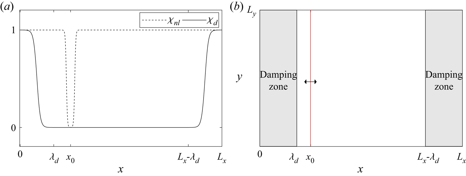
Figure 1. (a) Smooth functions  $\chi _{d}$ for damping zones (solid line) and $\chi _{nl}$ for spatial nonlinear adjustment (dashed line). (b) Computational domain with damping zones and influx line (red) for wave generation.
A potential theory is used assuming inviscid fluid and irrotational flow. The fluid velocity is expressed by the velocity potential  $\phi$, $\boldsymbol {V}=\boldsymbol {\nabla }\phi$. Assuming the fluid is incompressible, the continuity equation becomes the Laplace equation
 \begin{equation} \boldsymbol{\nabla} \boldsymbol{\cdot} \boldsymbol{\nabla} \phi = 0. \end{equation}
We consider periodic boundary conditions in the horizontal plane. The bottom boundary condition is
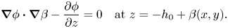 \begin{equation} \boldsymbol{\nabla}\phi \boldsymbol{\cdot} \boldsymbol{\nabla}\beta - \frac{\partial\phi}{\partial z} = 0 \quad \text{at}\ z={-}h_0+\beta(x,y). \end{equation}
 As pointed out in Zakharov (Reference Zakharov1968), the kinematic and dynamic nonlinear free surface boundary conditions can be written in terms of surface elevation  $\eta$ and surface potential $\phi _s=\phi (x,y,z=\eta,t)$
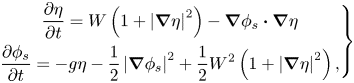 \begin{equation} \left.\begin{gathered} \frac{\partial \eta}{\partial t} = W \left( 1+ \left\vert \boldsymbol{\nabla} \eta \right\vert^2\right) - \boldsymbol{\nabla}\phi_s \boldsymbol{\cdot} \boldsymbol{\nabla}\eta \\ \frac{\partial\phi_s}{\partial t} ={-}g \eta -\frac{1}{2}\left\vert\boldsymbol{\nabla}\phi_s\right\vert^2 + \frac{1}{2}W^2\left(1+\left\vert\boldsymbol{\nabla}\eta\right\vert^2\right), \end{gathered}\right\} \end{equation}
where  $g$ is the acceleration of gravity and $W={\partial \phi }/{\partial z}\vert _{z=\eta }$ is the vertical velocity at the surface. The surface vertical velocity $W$ needs to be evaluated to solve the system. For flat bottom, an efficient pseudo-spectral method to calculate the surface vertical velocity $W$ in terms of $\eta$ and $\phi _s$ was initially introduced by Dommermuth & Yue (Reference Dommermuth and Yue1987) and West et al. (Reference West, Brueckner, Janda, Milder and Milton1987), and it has been known as the high-order spectral method (HOSM). Extension to variable depth was discussed in Gouin, Ducrozet & Ferrant (Reference Gouin, Ducrozet and Ferrant2016, Reference Gouin, Ducrozet and Ferrant2017). A brief summary of the HOSM for variable depth by Gouin et al. (Reference Gouin, Ducrozet and Ferrant2017) is presented in the following.
The velocity potential  $\phi$ is expressed as a truncated power series $\phi =\sum _{m=1}^M \phi ^{(m)}$ where $m$ is the nonlinear order of $\phi ^{(m)}$ and $M$ is the nonlinear order of the method which can be freely chosen. The velocity potential evaluated at the free surface $\phi _s$ is then expanded in a Taylor series around the still water level $z=0$.
For an uneven bottom, an additional velocity potential  $\phi _B$ is expressed as a truncated power series $\phi _B=\sum _{m=1}^M \phi _B^{(m)}$ and $\phi _B^{(m)}=\sum _{l=1}^{M_B}\phi _B^{(m,l)}$ where $M_B$ is the order for the bottom boundary condition which can be different from $M$ and can be freely chosen. Thus, the velocity potential $\phi ^{(m)}$ is expressed as the sum of two components
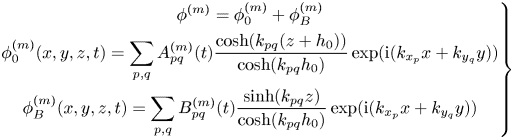 \begin{equation} \left.\begin{gathered} \phi^{(m)} = \phi_0^{(m)} + \phi_B^{(m)}\\ \phi_0^{(m)}(x,y,z,t) = \sum_{p,q} A_{pq}^{(m)}(t) \frac{\cosh(k_{pq}(z+h_0))}{\cosh(k_{pq}h_0)} \exp({{\rm i}(k_{x_p}x +k_{y_q}y)})\\ \phi_B^{(m)}(x,y,z,t) = \sum_{p,q} B_{pq}^{(m)}(t) \frac{\sinh(k_{pq}z)}{\cosh(k_{pq}h_0)} \exp({{\rm i}(k_{x_p}x +k_{y_q}y)}) \end{gathered}\right\} \end{equation}
with  $k_{x_p}=(p-{N_x}/{2}+1)({2{\rm \pi} }/{L_x})$ for $p=0,\ldots,N_x-1$, $k_{y_q}=(q-{N_y}/{2}+1)({2{\rm \pi} }/{L_y})$ for $q=0,\ldots,N_y-1$ and $k_{pq}=\sqrt {k_{x_p}^2+k_{y_q}^2}$. Here $N_x$ and $N_y$ are the number of wave components in the $x$ and $y$ directions, respectively. We choose $N_x$ and $N_y$ to be even numbers. We use $A_{pq}^{(m)}(t)$ and $B_{pq}^{(m)}(t)=\sum _{l=1}^{M_B}B_{pq}^{(m,l)}(t)$ to denote the modal amplitudes of $\phi _0^{(m)}$ and $\phi _B^{(m)}$, respectively. With the velocity potential in (2.4) and Taylor expansion of the bottom boundary condition in (2.2), we can calculate each $B_{pq}^{(m,l)}(t)$.
For evaluation of the vertical velocity at the surface,  $W$, a similar expansion series of surface potential is applied for the vertical velocity at the surface $W=\sum _{m=1}^{M}W^{(m)}$. Then, Taylor expansion around the still water level $z=0$ leads to a triangular system for $W^{(m)}$ to be solved iteratively. Once the vertical velocity at the surface $W^{(m)}$ has been computed, then the free surface elevation $\eta$ and surface potential $\phi _s$ can be marched in time through (2.3).
This method is based on a Taylor expansion of the bottom boundary condition with respect to the mean water depth and solved numerically by pseudo-spectral method. The bottom and its gradient need to be continuous to avoid any instabilities. For larger bottom variation  $\beta /h_0$, the error on the vertical velocity at the surface, $W$, becomes larger and the convergence is slower but still exists by increasing number of wave components and orders of the method $M$ and $M_B$. A detailed convergence study in one horizontal dimension with respect to the number of wave component $N_x$ and orders $M$ and $M_B$ is presented for variable depth in Gouin et al. (Reference Gouin, Ducrozet and Ferrant2016).
2.2. Wave generation and damping zones
For a flat bottom, the simulation can be initiated by specifying the surface elevation  $\eta$ and the surface potential $\phi _s$ at initial time $t=0$. The prescribed initial condition has to be periodic because of the pseudo-spectral method. For an uneven bottom, it is convenient to start simulations from rest ( $\eta =\phi _s=0$) and use a wave generator inside the domain. Embedded wave generation is implemented with spatial nonlinear adjustment as described in Lie, Adytia & van Groesen (Reference Lie, Adytia and van Groesen2014). To ensure the periodicity, a couple of damping zones of length $\lambda _d$ are also applied.
The dynamic equations with embedded wave generation and damping zones become
 \begin{equation} \left.\begin{gathered} \frac{\partial \eta}{\partial t} = RHS_{lin} + RHS_{nonlin}\chi_{nl} - c_d\eta\chi_d + S_{x_0}\\ \frac{\partial \phi_s}{\partial t} = RHS_{lin} + RHS_{nonlin}\chi_{nl} - c_d\phi_s\chi_d \end{gathered}\right\} \end{equation}
where  $RHS_{lin}$ and $RHS_{nonlin}$ are the linear and nonlinear parts of right-hand sides of the dynamic equations, $c_d$ is the damping coefficient, $S$ is the source term for embedded wave generation and $\chi _{nl}$ and $\chi _d$ are smooth functions. Illustration of the chosen functions for nonlinear adjustment and damping zones is shown in figure 1. In the damping zone, the solutions decay exponentially as $\textrm {e}^{-c_dT_d}$, where $T_d$ is the travel time of the wave in the damping zone. The value of the damping coefficient $c_d$ and the length of the damping zone $\lambda _d$ are coupled. As an example, for exponential decay of $10^{-3}\approx \textrm {e}^{-7}$, the length of the damping zone should be at least $\lambda _d=7V_g/c_d$, where $V_g$ is the group velocity.
2.3. Wave kinematics calculation
The HOSM calculates the surface vertical velocity  $W$ in terms of surface elevation $\eta$ and surface potential $\phi _s$. For wave kinematics calculation, it is convenient to use (2.4) directly after the modal amplitudes $A_{pq}$ and $B_{pq}$ are known. We refer this method as the direct method in this paper. We consider a solitary wave and Stokes waves on a flat bottom to check the validity of the direct method.
Solitary waves with amplitude over depth  $A/h=0.4$ and $A/h=0.6$ are chosen. We took the surface elevation and the surface potential for the solitary waves from the exact solution of the Euler equations by Dutykh & Clamond (Reference Dutykh and Clamond2014) as input to calculate the interior horizontal velocity with the direct method. Figure 2 shows the comparison of the horizontal velocity profile of solitary wave at the crest by the direct method and the reference solution from Dutykh & Clamond (Reference Dutykh and Clamond2014). For a rather extreme solitary wave $A/h=0.6$, the direct method gives inaccurate horizontal velocity close to the surface. For a milder case $A/h=0.4$, the accuracy of the direct method can be improved by increasing the nonlinear order.

Figure 2. Horizontal velocity profiles of solitary waves with (a)  $A/h=0.4$ and (b) $A/h=0.6$.
We consider a Stokes waves in deep water ( $kh=10$) with $ka=0.1$ and $ka=0.3$, where $a$ is the first-order amplitude, $k$ is the wavenumber and $h$ is the water depth. We use the fifth-order solution by Fenton (Reference Fenton1985) to obtain the surface elevation and surface potential. The surface potential is calculated from the fifth-order velocity potential at $z=\eta$, retaining fifth-order terms. Figure 3 shows the comparison of horizontal velocity under the wave crest by the direct method with Fenton's solution. For Stokes wave with steepness $ka=0.1$, the direct method gives a good agreement compared with Fenton's solution. Meanwhile, the horizontal velocity by the direct method starts to deviate from Fenton's solution close to the surface when the steepness is increased to $ka=0.3$.
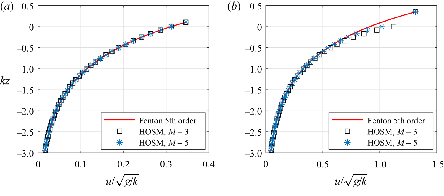
Figure 3. Horizontal velocity profiles of Stokes waves with (a)  $ka=0.1$ and (b) $ka=0.3$.
From both test cases, we see that the direct method is inaccurate to calculate the horizontal velocity near the surface for strongly nonlinear cases. However, the direct method is still valid down to the bottom and for low steepness parameter  $A/h$ in shallow water or $ka$ in deep water. This problem has been pointed out in Bateman, Swan & Taylor (Reference Bateman, Swan and Taylor2003) where the $H$ and $H_2$ operators were introduced. For flat bottom, the direct method is equivalent to the $H$ operator method. The $H_2$ operator method was proposed in Bateman et al. (Reference Bateman, Swan and Taylor2003) as a remedy. For varying bottom, the more advanced variational Boussinesq model was proposed to calculate the wave kinematics in Lawrence, Gramstad & Trulsen (Reference Lawrence, Gramstad and Trulsen2021a).
In the present paper, we focus on the interior horizontal fluid velocity where it is not close to the water surface or the bottom. Therefore, we still use the direct method because it is efficient and sufficiently accurate to study the evolution of the statistical properties of velocity field.
3. Statistical moments
We focus on the third- and fourth-order moments of the surface elevation and horizontal velocity, the skewness and the kurtosis, respectively. The skewness and the kurtosis of the surface elevation are defined as
 \begin{equation} \text{skewness} = \frac{\text{E}\left[\left(\eta - \text{E}[\eta] \right)^3\right]}{\sigma(\eta)^3},\quad \text{kurtosis} = \frac{\text{E}\left[\left(\eta - \text{E}[\eta] \right)^4\right]}{\sigma(\eta)^4}, \end{equation}
where  $\textrm {E}[\cdot ]$ denotes the expected value and $\sigma (\cdot )$ is the standard deviation. We have similar expressions for the horizontal velocity.
The skewness is a measure of the asymmetry of the distribution, whereas the kurtosis measures the dominance of the tails of the distribution. For a Gaussian distribution, the skewness is zero and the kurtosis is three. In the present study, we study the nonlinear effects by two-dimensional bathymetry that trigger non-Gaussian statistics indicated by the skewness and the kurtosis.
We use a Monte Carlo approach to estimate the statistical moments. We have performed numerical simulations multiple times with different incoming wave fields, i.e. wave fields generated from the same spectrum but with different random phases. From each simulation, we collect time series of surface elevation and horizontal velocity of length 100 $T_p$ in the domain of interest. The statistical moments are calculated by using time averaging first on the time series of length 100 $T_p$ then ensemble averaging from all different realisations.
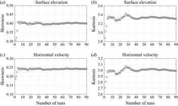
A convergence study of the ensemble-averaged statistical moments with respect to the number of random runs was performed. As an example, we run 90 different realisations of case 3 in irregular waves over a circular shoal in § 4.1. Figure 4 shows the convergence of skewness and kurtosis with respect to the number of runs at the centre of the circular shoal. From these 90 realisations, we choose  $n=10,20,30$ and $40$ random realisations and calculate the ensemble-averaged kurtosis of surface elevation. This process is repeated 100 times and we show the mean value, $\mu$, and the standard deviation, $\sigma$, of averaged kurtosis of surface elevation in figure 5. We decided that 40 realisations is sufficient to have reliable estimates of the skewness and kurtosis.
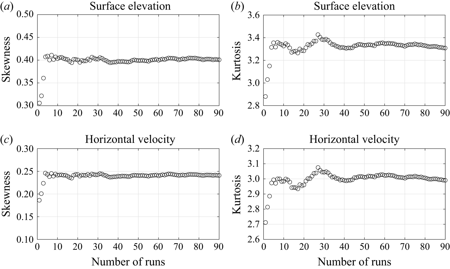
Figure 4. Convergence of the ensemble-averaged skewness and kurtosis of surface elevation and horizontal velocity at the centre of the circular shoal with respect to the number of runs.
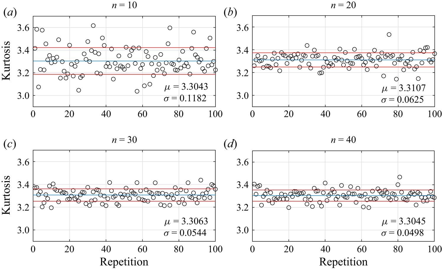
Figure 5. Averaged kurtosis of surface elevation from  $n=10,20,30$ and $40$ random different runs. Here $\mu$ is the mean value and $\sigma$ is the standard deviation from 100 repetitions.
4. Results
4.1. Irregular waves over a circular shoal
Long-crested irregular waves propagating over a circular shoal in computational domain with length 35 m and width 18 m is simulated by HOSM with truncation orders  $M=2$ and $M_B=7$. The length of the damping zones are $\lambda _d=5$ m at the left and right boundaries. The damping coefficient was set to $c_d = 1\,\textrm {s}^{-1}$. The wave generator is located inside the domain at $x=8$ m. The number of wave components in $x$ and $y$ directions are $N_x=512$ and $N_y=32$, respectively. The numerical simulation used similar bathymetry as the experiments of Chawla & Kirby (Reference Chawla and Kirby1996), but with a different radius. The horizontal velocity is calculated at $z=-0.04$ m. A sketch of the computational domain is given in figure 6.
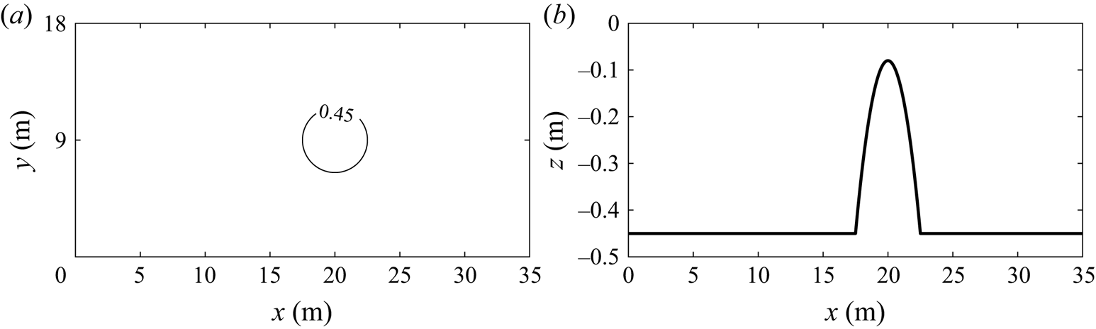
Figure 6. Bottom topography of circular shoal with radius 2.5 m: (a) bottom contour; (b) centreline depth.
The circular shoal has a radius of  $R_{shoal}$ and the centre is located at $x=20$ and $y=9$ m. The water depth on the shoal is given by
 \begin{equation} h = h_0+R_{sphere}-0.37-\sqrt{R_{sphere}^2-(x-20)^2-(y-9)^2}, \end{equation}
where  $R_{sphere}=(R_{shoal}^2+0.37^2) / (2 \times 0.37)$, $h_0=0.45$ m is the constant water depth and the water depth on top of the shoal is $h_{top}=0.08$ m. All numbers in (4.1) and $R_{sphere}$ have unit of length meters (m).
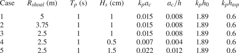
The incoming wave field has a JONSWAP spectrum with peak period  $T_p=1$ s, significant wave height $H_s$ and peak enhancement factor $\gamma =3.3$. The non-dimensional depth $k_ph$ on the flat bottom part is 1.89 and on top of the shoal it is 0.6, where $k_p$ is the corresponding peak wavenumber calculated from the peak period based on the linear dispersion relation. The steepness parameters are $k_pa_c=0.0149$ and $a_c/h_0=0.0079$, where $a_c=\sqrt {2}\sigma$ is the characteristic amplitude and $\sigma ={H_s}/4$ is the standard deviation of the surface elevation. The characteristic wavelength $\lambda _p=2{\rm \pi} /k_p$ is 1.49 m. The parameters are summarised in table 1. The evolution of the power spectral density of the surface elevation and the horizontal velocity is included in the Appendix for Case 3.
Table 1. Key parameters for irregular waves over a circular shoal simulation.
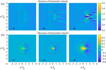
Figures 7 and 8 show the statistics of the surface elevation and the horizontal velocity for irregular waves propagating over a circular shoal with different radii. The skewness has a local maximum on top of the shoal but not in the centre of the shoal, and has a local minimum on the lee side of the shoal. The skewness of the surface elevation and the horizontal velocity have the same trend. However, the surface elevation and the horizontal velocity have completely different behaviours for the kurtosis. The kurtosis of the surface elevation has a local maximum on top of the shoal, whereas the horizontal velocity has two local maxima of kurtosis at different locations on the lee side of the shoal. It is also noted that the kurtosis of surface elevation has other local maxima on the lee side of the shoal.
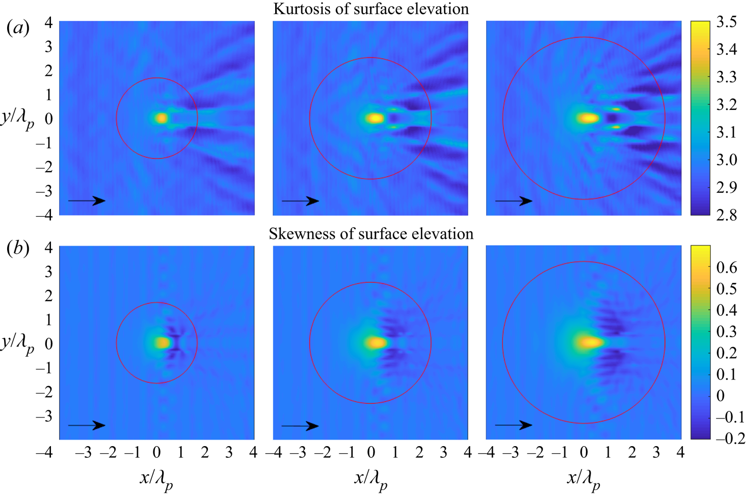
Figure 7. (a) Kurtosis of surface elevation and (b) skewness of surface elevation for irregular waves over a circular shoal with  $R_{shoal}=2.5$, 3.75 and 5 m (from left to right). The red circle indicates the edge of the shoal at constant depth.
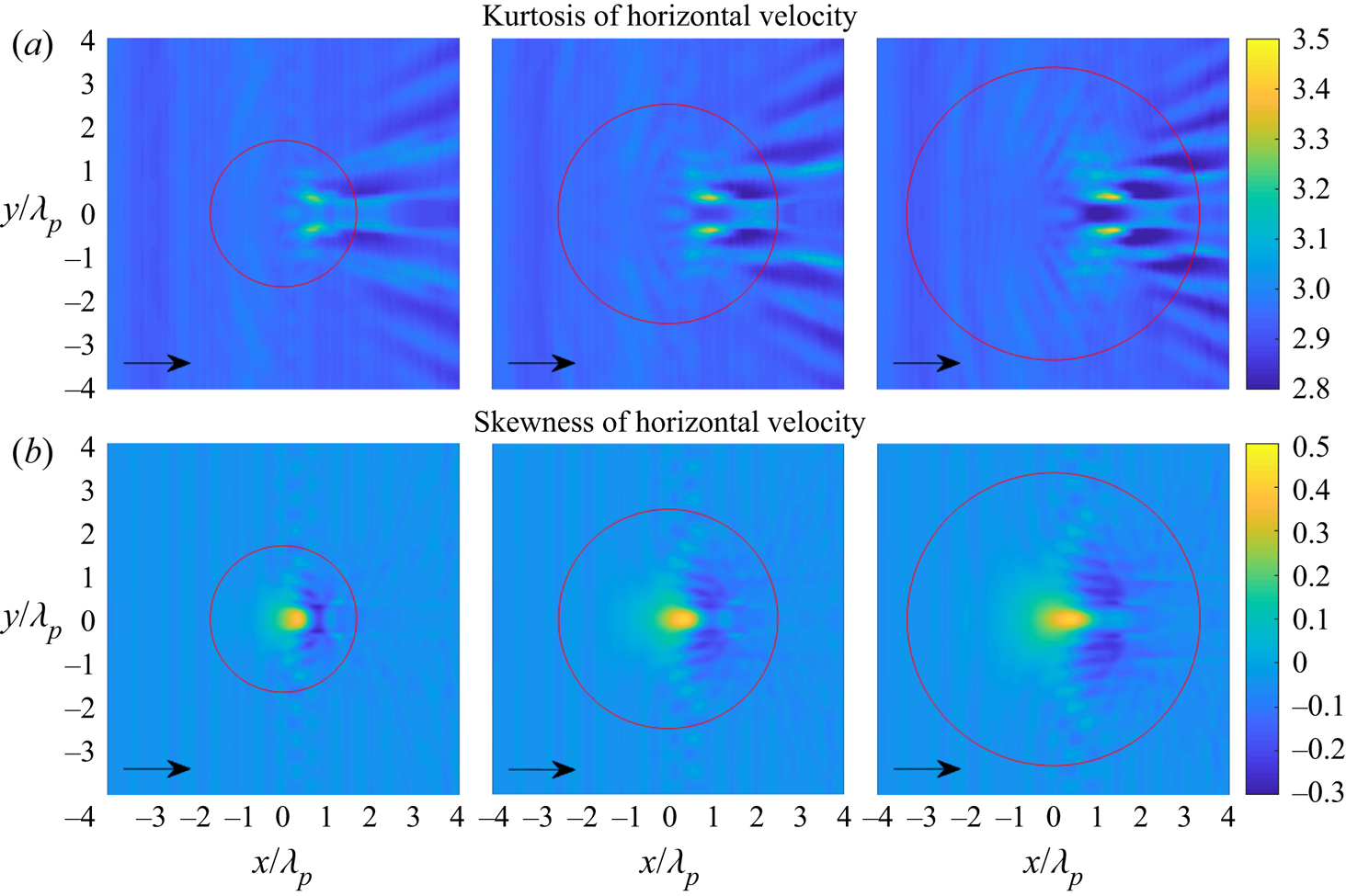
Figure 8. (a) Kurtosis of horizontal velocity and (b) skewness of horizontal velocity for irregular waves over a circular shoal with  $R_{shoal}=2.5$, 3.75 and 5 m (from left to right). The red circle indicates the edge of the shoal at constant depth.
Figures 9 and 10 show the statistics of the surface elevation and the horizontal velocity for irregular waves propagating over a circular shoal with same radius  $R_{shoal}=2.5$ m, but with different significant wave height $H_s$. The skewness of surface elevation and horizontal velocity still have the same trend with a local maximum on top of the shoal and a local minimum on the lee side of the shoal. For the highest significant wave height $H_s=1.5$ cm, it is observed that the kurtosis of surface elevation has local maxima on top of the shoal and on the lee side of the shoal. Meanwhile, the kurtosis of horizontal velocity only has local maxima on the lee side of the shoal.
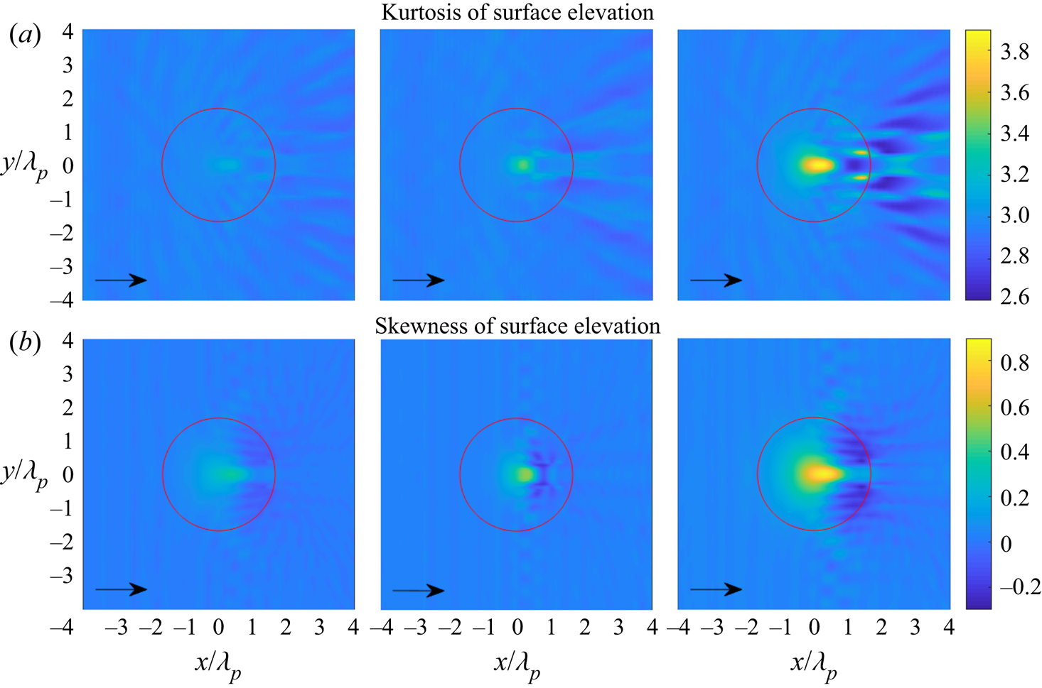
Figure 9. (a) Kurtosis of surface elevation and (b) skewness of surface elevation for irregular waves over a circular shoal with  $H_s=0.5$, 1 and 1.5 cm (from left to right). The red circle indicates the edge of the shoal at constant depth.
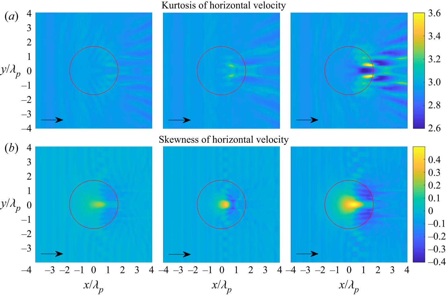
Figure 10. (a) Kurtosis of horizontal velocity and (b) skewness of horizontal velocity for irregular waves over a circular shoal with  $H_s=0.5$, 1 and 1.5 cm (from left to right). The red circle indicates the edge of the shoal at constant depth.
4.2. Irregular waves over a semicircular step
Long-crested irregular waves propagating over a submerged bar with a semicircular step in a periodic computational domain with length 40 m and width 18 m is simulated by the HOSM with same setup as in § 4.1.
We consider two types of bottom topography in this subsection. First, a submerged bar similar to the experiment by Trulsen et al. (Reference Trulsen, Raustøl, Jorde and Rye2020), but with a semicircular step on the lee side, see figure 11. Second, a submerged bar with a semicircular step on the front and longer distance in the shallower part, see figure 12. The radius of the semicircle is 3 m. The water depth  $h_0$ on the deeper part is 0.53 m and the water depth on the shallower part is 0.11 m. The horizontal velocity is calculated at $z=-0.055$ m.
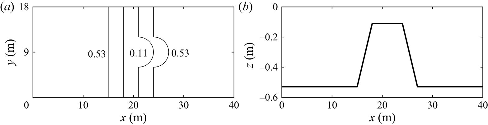
Figure 11. Bottom topography of submerged bar with semicircular step behind: (a) bottom contours; (b) centreline depth.
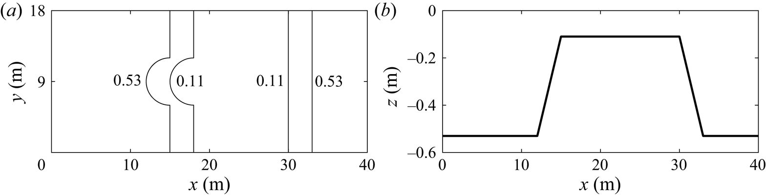
Figure 12. Bottom topography of submerged bar with semicircular step in front: (a) bottom contours; (b) centreline depth.
For both cases, the incoming wave field has a JONSWAP spectrum with peak period  $T_p=1.1$ s, significant wave height $H_s=2.5$ cm and peak enhancement factor $\gamma =3.3$ similar to run 3 in Trulsen et al. (Reference Trulsen, Raustøl, Jorde and Rye2020). The non-dimensional depth $k_p h$ on the deeper part is 1.85 and on the shallower part is 0.64. The steepness parameters are $k_pa_c=0.0123$ and $a_c/h_0=0.0067$. The characteristic wavelength $\lambda _p=2{\rm \pi} /k_p$ is 1.8 m.
Figures 13 and 14 show the skewness and kurtosis of the surface elevation and the horizontal velocity for the submerged bar with a semicircular step on the lee side and on the front, respectively.
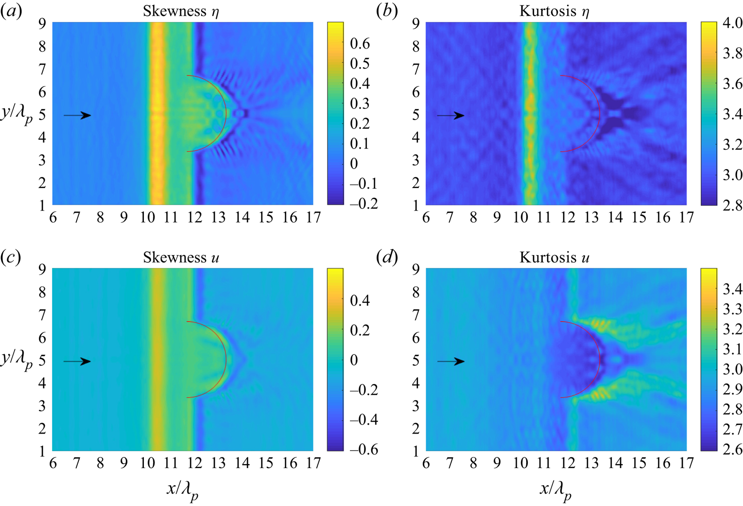
Figure 13. (a), (c) Skewness and (b), (d) kurtosis of (a), (b) surface elevation and (c), (d) horizontal velocity of irregular waves propagating over a submerged bar with a semicircular step behind. The red curve indicates the edge of the semicircular step on the shallower depth.
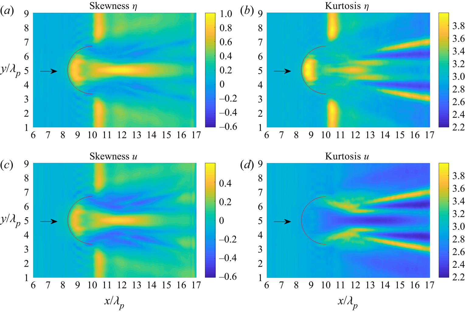
Figure 14. (a), (c) Skewness and (b), (d) kurtosis of (a), (b) surface elevation and (c), (d) horizontal velocity of irregular waves propagating over a submerged bar with a semicircular step in front. The red curve indicates the edge of the semicircular step on the shallower depth.
In figure 13, the skewness of the surface elevation and the horizontal velocity have the same behaviour. The skewness has local maximum on the shallower part of the bar and has a local minimum on the downslope. The kurtosis of surface elevation also has local maximum on the shallower part of the bar. Meanwhile, the kurtosis of horizontal velocity has different behaviour. There are increases in kurtosis of horizontal velocity on the downslope of semicircular step on the lee side.
In figure 14, the skewness of the surface elevation and the horizontal velocity has the same trend. The skewness has a local maximum after the edge of the upslope on the shallower part and also after some distance on the shallower part along the centreline. The kurtosis of the surface elevation has a local maximum after the edge of the upslope on the shallower part and also after some distance on the shallower part. On the other hand, the kurtosis of horizontal velocity has local maxima at different locations than the surface elevation. We notice there is a pattern for the kurtosis after some distance from the semicircular step on the front.
5. Discussion
Our numerical simulations confirm that non-uniform bathymetry can produce non-Gaussian statistics for both surface elevation and horizontal velocity. The statistical properties of the surface elevation and horizontal velocity can be different when the waves propagate over a varying bathymetry.
For irregular waves propagating over a circular shoal, the skewness of the surface elevation and horizontal velocity have local maxima on top of the shoal followed by a local minimum on the lee side of the shoal. The kurtosis of the surface elevation has a local maximum on top the shoal. This result is similar to the one-dimensional case reported experimentally in Trulsen et al. (Reference Trulsen, Raustøl, Jorde and Rye2020) and numerically in Lawrence et al. (Reference Lawrence, Trulsen and Gramstad2021b). Unexpectedly, the kurtosis of surface elevation can have other local maxima on the lee side of the shoal and the kurtosis of the horizontal velocity also has two local maxima on the lee side of the shoal. It seems the two-dimensional effects from bottom topography such as refraction and diffraction influence the kurtosis of the surface elevation and the horizontal velocity.
For our cases with different bottom topography, a submerged bar with a semicircular step on the lee side acts similar to a focusing lens where the waves propagate from shallower to deeper water. The kurtosis of horizontal velocity has a significant increase not in the centre but on the left and right side from the direction of incoming waves of semicircular step as shown in figure 13. On the other hand, a submerged bar with a semicircular step on the front also acts similar to a focusing lens but from deeper to shallower water. After some distance from the edge of the semicircular step, in the area of the focal zone, there is a huge increase in the skewness of the surface elevation and the horizontal velocity. The kurtosis of the surface elevation has a local maximum around the centreline, whereas the kurtosis of the horizontal velocity has positive excess kurtosis not close to the centreline as shown in figure 14.
Our results suggest that the two-dimensional bathymetry affects the skewness and the kurtosis for both surface elevation and horizontal velocity.
6. Summary and conclusion
We have performed a numerical study of the statistical properties of the surface elevation and the velocity field of long-crested irregular waves propagating over a two-dimensional bathymetry with a Monte Carlo approach. The statistical properties were studied in terms of evolution of the skewness and the kurtosis. The numerical simulations were performed using the HOSM for varying bottom from Gouin et al. (Reference Gouin, Ducrozet and Ferrant2017). We considered two types of bathymetry: a circular shoal and submerged bar with a semicircular step.
For our circular shoal, the depth transition is from  $k_ph=1.89$ to $k_ph=0.6$. It has been found that the skewness of surface elevation and horizontal velocity have the same trend: a local maximum on top of the shoal and a local minimum on the lee side of the shoal. However, the kurtosis of surface elevation can have a local maximum on top of the shoal and local maxima on the lee side of the shoal. Meanwhile, the kurtosis of horizontal velocity only has two local maxima on the lee side of the shoal.
For our submerged bar with a semicircular step, the depth transition is from  $k_ph=1.85$ to $k_ph=0.64$. Without the semicircular step, the submerged bar itself is similar to the experiment by Trulsen et al. (Reference Trulsen, Raustøl, Jorde and Rye2020). We first considered submerged bar with a semicircular step on the lee side. In the area of the semicircular step on the lee side, the kurtosis of horizontal velocity increases at two locations similar to the previous case of a circular shoal. Second, we considered a submerged bar with a semicircular step on the front and longer distance in the shallower part. We have found that the skewness of the surface elevation and horizontal velocity have a significant increase after the edge of the upslope and also after some distance on the shallower part along the centreline. The kurtosis of the surface elevation has local maxima just after the edge of the upslope and after some distance on the shallower part. Meanwhile, the kurtosis of the horizontal velocity has local maxima not close to the centreline.
We conclude that two-dimensional bathymetry can trigger a significant increase in both skewness and kurtosis of surface elevation and horizontal velocity. The skewness of surface elevation and horizontal velocity have similar behaviour but the kurtosis of surface elevation and horizontal velocity can have completely different behaviours.
Declaration of interests
The authors report no conflict of interest.
Appendix
Figure 15 shows the power spectral density of the surface elevation and the horizontal velocity for case 3 with irregular waves propagating over a circular shoal. The power spectral density is calculated from an ensemble average of 40 different realisations.
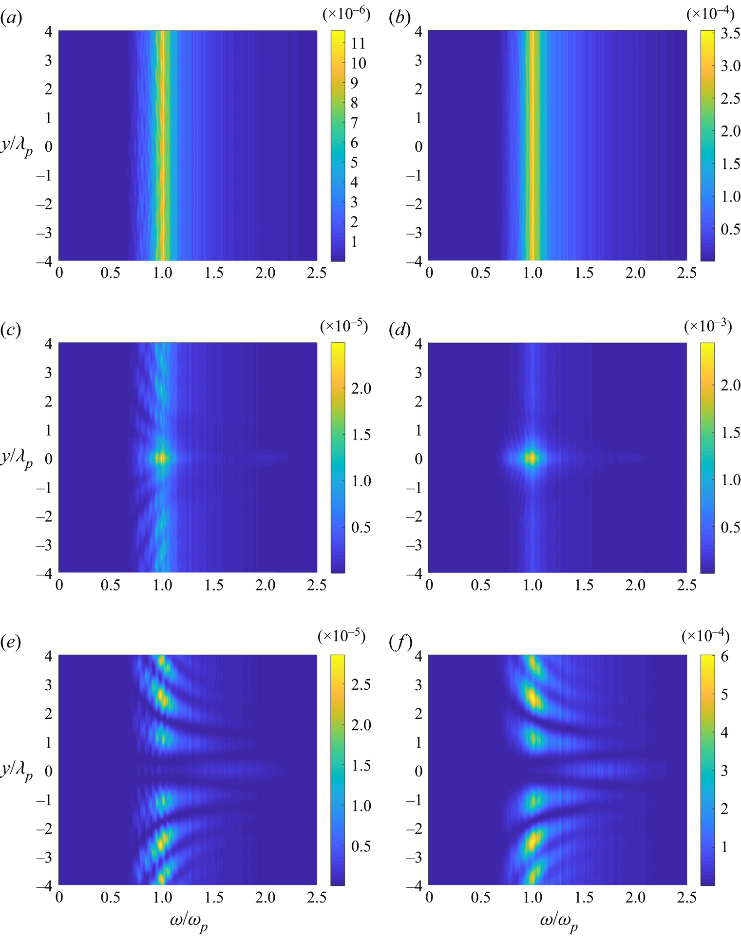
Figure 15. (a), (c), (e) Power spectral density of the surface elevation and (b), (d), (f) horizontal velocity of case 3 with irregular waves propagating over a shoal at  $x=15$ m (before the shoal, a and b), $x=20$ m (centre of the shoal, c and d) and $x=25$ m (after the shoal, e and f).


 Open access