


Crossref Citations
This article has been cited by the following publications. This list is generated based on data provided by Crossref.
Chen, Nan
and
Li, Yingda
2021.
BAMCAFE: A Bayesian machine learning advanced forecast ensemble method for complex turbulent systems with partial observations.
Chaos: An Interdisciplinary Journal of Nonlinear Science,
Vol. 31,
Issue. 11,
Zhang, Ziheng
and
Chen, Nan
2021.
Parameter Estimation of Partially Observed Turbulent Systems Using Conditional Gaussian Path-Wise Sampler.
Computation,
Vol. 9,
Issue. 8,
p.
91.
Hoffman, Johan
2021.
Energy stability analysis of turbulent incompressible flow based on the triple decomposition of the velocity gradient tensor.
Physics of Fluids,
Vol. 33,
Issue. 8,
Yan, Zheng
Fu, Yaowei
Wang, Lifeng
Yu, Changping
and
Li, Xinliang
2022.
Effect of chemical reaction on mixing transition and turbulent statistics of cylindrical Richtmyer–Meshkov instability.
Journal of Fluid Mechanics,
Vol. 941,
Issue. ,
Chen, Nan
Li, Yingda
and
Liu, Honghu
2022.
Conditional Gaussian nonlinear system: A fast preconditioner and a cheap surrogate model for complex nonlinear systems.
Chaos: An Interdisciplinary Journal of Nonlinear Science,
Vol. 32,
Issue. 5,
Mou, Changhong
Chen, Nan
and
Iliescu, Traian
2023.
An efficient data-driven multiscale stochastic reduced order modeling framework for complex systems.
Journal of Computational Physics,
Vol. 493,
Issue. ,
p.
112450.
Shen, Weiyu
Yao, Jie
Hussain, Fazle
and
Yang, Yue
2023.
Role of internal structures within a vortex in helicity dynamics.
Journal of Fluid Mechanics,
Vol. 970,
Issue. ,
Xiong, Xue-Lu
Laima, Shujin
Li, Hui
and
Zhou, Yi
2024.
Self-similarity in single-point turbulent statistics across different quadrants in turbulent rotor wakes.
Physical Review Fluids,
Vol. 9,
Issue. 5,
Granero Belinchon, Carlos
and
Cabeza Gallucci, Manuel
2024.
A multiscale and multicriteria generative adversarial network to synthesize 1-dimensional turbulent fields.
Machine Learning: Science and Technology,
Vol. 5,
Issue. 2,
p.
025032.
1. Introduction
A central challenge in the theory of turbulence is to resolve the precise mechanism by which energy is dissipated in the limit of very high Reynolds number ${{Re}}\gg 1$. In homogeneous turbulence, the mean rate of dissipation of energy $\epsilon$ is given by $\epsilon = \nu \left \langle \boldsymbol {\omega } ^{2}\right \rangle$. Here, $\nu$ is the kinematic viscosity of the fluid, $\boldsymbol {\omega } (\boldsymbol {x}, t)=\boldsymbol {\nabla } \times \boldsymbol {u}(\boldsymbol {x}, t)$ is the vorticity field, u is the velocity field and the angular brackets $\left \langle \cdots \right \rangle$ denote a space average. In the widely accepted, although simplistic, scenario of Kolmogorov (Reference Kolmogorov1941), the turbulence acquires its mean kinetic energy $\left \langle \boldsymbol {u}^{2}\right \rangle /2= u_{0}^{2}/2$ on a scale $\ell _{0}$ at a rate $\epsilon \sim u_{0}^{3}/\ell _{0}$; this energy cascades down through the ‘inertial range’ of scales to the Kolmogorov scale $\ell _{\nu }\sim (\epsilon /\nu ^{3})^{1/4}\sim {{Re}} ^{-3/4}\ell _{0}$, below which it is dissipated by viscosity. On dimensional grounds, the all-important parameter $\epsilon$ determines the energy spectrum $E(k)=C \epsilon ^{2/3}k^{-5/3}$ in the inertial range, where $C$ is supposedly a universal constant and k is the wavenumber. The vorticity spectrum $k^{2}E(k)$ thus rises like $k^{1/3}$ through the inertial range, peaking at a wavenumber k of order $k_{\nu }=\ell _{\nu }^{-1}$, consistent with $\left \langle \boldsymbol {\omega } ^{2}\right \rangle \sim \epsilon /\nu$. The fundamental process of vortex stretching is responsible for the cumulative intensification of vorticity on ever-decreasing length scales.
Following Kolmogorov (Reference Kolmogorov1962), it has been known for some time from direct numerical simulations that this process of vorticity intensification is extremely intermittent (see, for example, Ishihara et al. Reference Ishihara, Kaneda, Yokokawa, Itakura and Uno2007). With decreasing scale, the vorticity distribution becomes more and more concentrated in singular structures that look like highly distorted sheets or filaments of vorticity. The sheets have a natural tendency to break up into filaments by elliptic and/or Kelvin–Helmholtz instabilities (McKeown et al. Reference McKeown, Ostilla-Monico, Pumir, Brenner and Rubinstein2018). Such vortex filaments were first detected experimentally by Douady, Couder & Brachet (Reference Douady, Couder and Brachet1991), intermittent in both space and time (see also Rusaouën, Rousset & Roche (Reference Rusaouën, Rousset and Roche2017) for similar observations in liquid helium).
2. Most extreme events of local energy transfer
An important advance has now been made in the detection of near-singular structures in a turbulent flow that is driven by counter-rotating propellors in the ‘von Kármán’ configuration (Debue et al. Reference Debue, Valori, Cuvier, Daviaud, Foucaut, Laval, Wiertel, Padilla and Dubrulle2021; hereafter Reference Debue, Valori, Cuvier, Daviaud, Foucaut, Laval, Wiertel, Padilla and DubrulleDVC). These propellors drive a mean flow with a non-zero helicity that is presumably inherited by the turbulence. By the use of tomographic particle velocimetry, the authors have identified ‘extreme events of local energy transfer’, and have determined the structure of the local velocity and vorticity fields in each case. The Reynolds number based on the propellor geometry and rotation rate varied over the range $6.3\times 10^{3}$ to $3.1\times 10^{5}$; at the lower end of this range, it was possible to resolve structures on the dissipative length scale $\ell _{\nu } \sim 1.4\ \textrm {mm}$, whereas at the upper end only the inertial range was accessible.
Classification of extreme events has been based by Reference Debue, Valori, Cuvier, Daviaud, Foucaut, Laval, Wiertel, Padilla and DubrulleDVC on the non-zero invariants of the velocity-gradient tensor $S_{ij}=\partial u_{i}/\partial x_{j}$, defined by $Q(\boldsymbol {x})=- (S_{ij}S_{ji})/2, R(\boldsymbol {x})=-\text {det}[S_{ij}]$. If $M(R,Q)\equiv 27 R^{2}+4 Q^{3}<0$, the three eigenvalues of $S_{ij}$ are real, and local irrotational strain dominates over vorticity. If
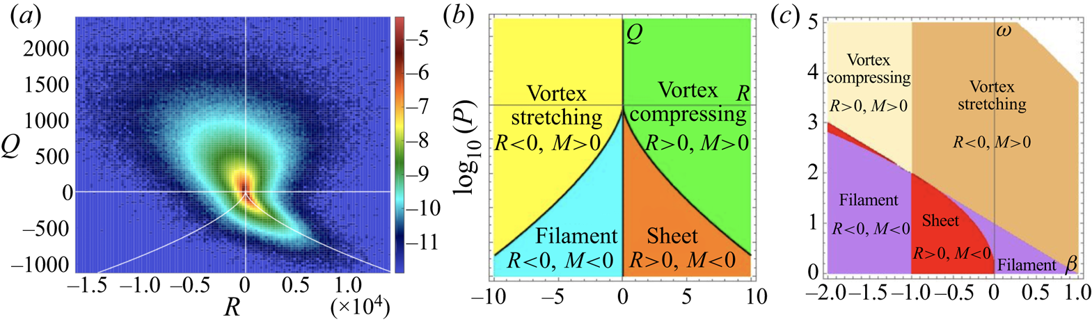
  $M>0$, one eigenvalue is real and the other two are complex conjugates, so vorticity dominates and streamlines are locally spiral or helical in character. Figure 1(a) reproduces figure 4(a) from Reference Debue, Valori, Cuvier, Daviaud, Foucaut, Laval, Wiertel, Padilla and DubrulleDVC: in this, the tear-drop region shows where, in the $\{R,Q\}$ plane, most extreme events are found (see also their figure 5(a), not shown here). Figure 1(b) shows the basic structure of this figure, in which this plane is separated into four regions in which topologically distinct structures were identified: vortex stretching; vortex compressing; sheets; and filaments.
Figure 1. (a) Reproduction of figure 4(a) from Reference Debue, Valori, Cuvier, Daviaud, Foucaut, Laval, Wiertel, Padilla and DubrulleDVC showing the joint p.d.f. (probability density function) of $R$ and $Q$, with dark red representing the maximum probability; the tear-drop region is the location where most extreme events are found, as shown in their figure 5(a) (not shown here); (b) the four regions of the same plane in which topologically distinct structures, as indicated, were identified; the cusped curve is $M(R,Q)\equiv 27 R^{2}+4 Q^{3}=0$; (c) corresponding divisions of the $\{\beta ,\omega _{0}\}$ plane, when the local velocity field takes the idealised form $\boldsymbol {u}=(-\alpha x- (\omega _{0} y)/2,-\beta y + (\omega _{0} x)/2,(\alpha +\beta )z)$ (with $\alpha =1$), as on the axis of a Burgers-type vortex.
Reference Debue, Valori, Cuvier, Daviaud, Foucaut, Laval, Wiertel, Padilla and DubrulleDVC found that the most extreme events of local energy transfer occurred in the vortex-stretching and vortex-compressing regions. It may be helpful to interpret this finding with reference to a simple vortical flow of the form
where $r^{2} =x^{2} +y^{2}$, this vortex being stretched by the non-axisymmetric strain field
At high vortex Reynolds number, such a vortex remains axisymmetric at leading order (Moffatt, Kida & Ohkitani Reference Moffatt, Kida and Ohkitani1994). On the vortex axis $r=0$, the components of the matrix $\{S_{ij}\}$ are
and the corresponding expressions for $Q$,
$Q$,  $R$ and $M$ take the simplified form
and
Taking $\alpha =1$, figure 1(c) shows the subdivisions of the $\{\beta ,\omega _{0}\}$ plane corresponding to those of figure 1(b). As might be expected, the ‘vortex-stretching’ region is a sub-region of the half-plane $\alpha +\beta >0$.
3. Three topological structures – or three in one?
Reference Debue, Valori, Cuvier, Daviaud, Foucaut, Laval, Wiertel, Padilla and DubrulleDVC found further that their extreme events were associated with three apparently different topological structures, which they describe as ‘screw vortex’, ‘roll vortex’ and ‘U-turn’; sample streamlines are shown in their figures 7(a,b) and 8(a), respectively. They recognise that these structures ‘may correspond to a single structure seen at different times or in different frames of reference’. This is an issue that can again be probed through consideration of an explicit vortex-stretching flow. We first replace (2.2) by the modified strain field
with
This flow, which satisfies $\boldsymbol {\nabla }\boldsymbol {\cdot } \boldsymbol {U}_{s}=0$, $\boldsymbol {\nabla }\times \boldsymbol {U}_{s}\ne 0$, could be produced by a system of secondary vortices near the ‘primary vortex’ (2.1a,b). When $\alpha +\beta >0$, it gives positive stretching for $|z| < 2.33$, negative (i.e. compression) for $|z| > 2.33$. (In this way, vortex stretching may always be coupled with adjacent vortex compression, thus explaining the surprisingly high probability of ‘vortex compressing’ in the p.d.f. plot of figure 1a.) Particle paths (i.e. instantaneous streamlines) of this flow combined with the primary vortex flow (2.1a,b) starting from any given point $\boldsymbol {X}(0)$ can be computed from the associated dynamical system $\text {d} \boldsymbol {X}/\text {d}t =\boldsymbol {u}_{v}(\boldsymbol {X})+\boldsymbol {U}_{s}(\boldsymbol {X})$. Their structure depends on the chosen point $\boldsymbol {X}(0)$ and on the frame of reference.
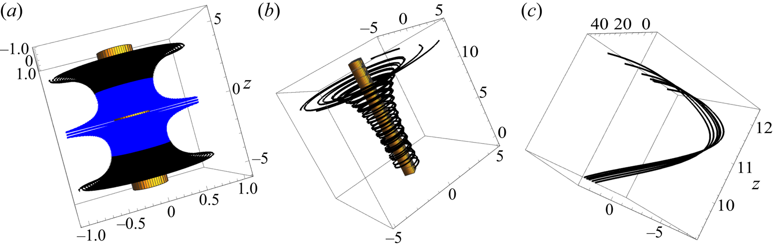
Three examples are shown in figure 2. Here, I have chosen $\alpha =0.001, \beta =0.0005, \omega _{0}=0.2$, so that
and (for $|z|<2.33$) we are indeed in the vortex-stretching regime $R<0, M>0$. Although computed from the same velocity field in the same vortex neighbourhood, these streamline patterns nevertheless look quite different: figures 2(a), 2(b) and 2(c) have structures comparable with those of Reference Debue, Valori, Cuvier, Daviaud, Foucaut, Laval, Wiertel, Padilla and DubrulleDVC's screw vortex, roll vortex and U-turn, respectively. Thus care is certainly needed in classifying such observed structures, for which vorticity is presumably a more robust topological feature than velocity.
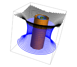
Figure 2. Streamlines computed from the dynamical system $\text {d} \boldsymbol {X}/\text {d}t =\boldsymbol {u}_{v}(\boldsymbol {x})+\boldsymbol {U}_{s}(\boldsymbol {x})$; $\alpha =0.001, \beta =0.0005, \omega _{0}=0.2$; the vorticity contour $\omega /\omega _{0}=0.3$ is shown in brown, and, as in Reference Debue, Valori, Cuvier, Daviaud, Foucaut, Laval, Wiertel, Padilla and DubrulleDVC, streamlines are shown in blue when approaching the vortex, black when leaving it; (a) $\boldsymbol {X}(0)=(1, 0, {\pm }0.01)$ and $(1, 0, {\pm }0.2)$; (b) the same streamlines viewed in a frame of reference moving with velocity $(0, 0, -0.01); \boldsymbol {X}(0)=(1, 0, {\pm }0.2)$; (c) eight streamlines starting from points close to $\boldsymbol {X}(0)=(2.87, 0, 0)$ and plotted for dimensionless time $1000\le t \le 4000$ when they first ‘encounter’ the vortex.
Declaration of interest
The author reports no conflict of interest.