


1 Introduction
Enhancing the heat transport in flows is desirable in many practical applications. To achieve this in systems with natural convection, several approaches have been adopted. For example, in vertical natural convection, the usage of fins or riblets is proven to increase the heat flux (Shakerin, Bohn & Loehrke Reference Shakerin, Bohn and Loehrke1988). In Rayleigh–Bénard convection (Ahlers, Grossmann & Lohse Reference Ahlers, Grossmann and Lohse2009; Lohse & Xia Reference Lohse and Xia2010) heat transfer enhancement can be achieved by tuning the boundary conditions to aid the formation of large-scale rolls or coherent structures (Chong et al. Reference Chong, Huang, Kaczorowski and Xia2015), or by introducing wall roughness elements (e.g. Roche et al. Reference Roche, Castaing, Chabaud and Hébral2001; Tisserand et al. Reference Tisserand, Creyssels, Gasteuil, Pabiou, Gibert, Castaing and Chilla2011; Xie & Xia Reference Xie and Xia2017; Zhu et al. Reference Zhu, Stevens, Verzicco and Lohse2017). While these methods have been widely used to optimise convective transport, they pose limits on the maximum achievable heat flux in moderate to high Rayleigh number flows.
An alternative is the injection of bubbles in the flow, which indeed enhances the heat transport considerably (Deckwer Reference Deckwer1980). In general, the bubbles can be injected in a quiescent liquid phase (‘pseudo-turbulent’ flow: Risso & Ellingsen Reference Risso and Ellingsen2002; Mercado Martínez et al. Reference Mercado Martínez, Chehata Gǿmez, Van Gils, Sun and Lohse2010; Riboux, Risso & Legendre Reference Riboux, Risso and Legendre2010; Roghair et al. Reference Roghair, Martinez Mercado, Van Sint Annaland, Kuipers, Sun and Lohse2011) or in an already turbulent liquid phase (turbulent bubbly flow: Rensen, Luther & Lohse Reference Rensen, Luther and Lohse2005; Van Den Berg et al. Reference Van Den Berg, Luther, Mazzitelli, Rensen, Toschi and Lohse2006; van Gils et al. Reference van Gils, Narezo Guzman, Sun and Lohse2013; Prakash et al. Reference Prakash, Martínez Mercado, van Wijngaarden, Mancilla, Tagawa, Lohse and Sun2016; Spandan et al. Reference Spandan, Ostilla-Mónico, Verzicco and Lohse2016). It is known that the motion of injected bubbles induces mixing of warm and cold parcels of the liquid phase, which in industrial applications where heat transport is coupled with the bubbly flow can lead to a 100 times greater heat transfer coefficient when compared to the single-phase case (Deckwer Reference Deckwer1980). Therefore there is a practical benefit from a better understanding of the heat transport in bubbly flows as this enables better design and optimisation of the industrial processes. As a result, the effect of bubbles on heat transfer has been subject of several experimental and numerical studies in the past.
The bubbles can be injected in a system with natural or forced convection. Early studies which focused on forced convective heat transfer in bubbly flows (Sekoguchi, Nakazatomi & Tanaka Reference Sekoguchi, Nakazatomi and Tanaka1980; Sato, Sadatomi & Sekoguchi Reference Sato, Sadatomi and Sekoguchi1981a ,Reference Sato, Sadatomi and Sekoguchi b ) showed that the bubbles modify the temperature profile and that higher void fractions close to the heated wall lead to an enhanced heat transfer. In a more recent numerical study on forced convective heat transfer in turbulent bubbly flow in vertical channels, Dabiri & Tryggvason (Reference Dabiri and Tryggvason2015) showed that both nearly spherical and deformable bubbles, improve the heat transfer rate. They found that a 3 % volume fraction of bubbles increases the Nusselt number by 60 %.
Studies of natural convection in bubbly flow have been performed mostly by introducing micro-bubbles (Kitagawa et al.
Reference Kitagawa, Kosuge, Uchida and Hagiwara2008; Kitagawa, Uchida & Hagiwara Reference Kitagawa, Uchida and Hagiwara2009) and sub-millimetre bubbles (Kitagawa & Murai Reference Kitagawa and Murai2013) close to the heated wall. Among these, the micro-bubbles (mean bubble diameter
 $d_{bub}=0.04~\text{mm}$
) showed higher heat transfer enhancement as compared to sub-millimetre bubbles (
$d_{bub}=0.04~\text{mm}$
) showed higher heat transfer enhancement as compared to sub-millimetre bubbles (
 $d_{bub}=0.5~\text{mm}$
) (Kitagawa & Murai Reference Kitagawa and Murai2013). The authors stated that this occurred because the micro-bubbles form large bubble swarms which rise close to the wall and enhance mixing in the direction of the temperature gradient, while sub-millimetre bubbles, owing to their weak wake and low bubble number density, resulted in limited mixing. In contrast, in the case of bubbles with diameter of a few millimetres, the wake of individual bubbles and vortex shedding behind the bubbles play significant roles in the heat transfer enhancement (Kitagawa & Murai Reference Kitagawa and Murai2013). Tokuhiro & Lykoudis (Reference Tokuhiro and Lykoudis1994) experimentally studied the effects of
$d_{bub}=0.5~\text{mm}$
) (Kitagawa & Murai Reference Kitagawa and Murai2013). The authors stated that this occurred because the micro-bubbles form large bubble swarms which rise close to the wall and enhance mixing in the direction of the temperature gradient, while sub-millimetre bubbles, owing to their weak wake and low bubble number density, resulted in limited mixing. In contrast, in the case of bubbles with diameter of a few millimetres, the wake of individual bubbles and vortex shedding behind the bubbles play significant roles in the heat transfer enhancement (Kitagawa & Murai Reference Kitagawa and Murai2013). Tokuhiro & Lykoudis (Reference Tokuhiro and Lykoudis1994) experimentally studied the effects of
 $2{-}4~\text{mm}$
diameter inhomogeneously injected nitrogen bubbles on laminar and turbulent natural convection heat transfer from a vertical heated plate in mercury. They reported a twofold increase in the heat transfer coefficient as compared to the case without bubbles. Similarly, Deen & Kuipers (Reference Deen and Kuipers2013) showed in their numerical study that a few high Reynolds number bubbles rising in quiescent liquid could increase the local heat transfer between the liquid and a hot wall.
$2{-}4~\text{mm}$
diameter inhomogeneously injected nitrogen bubbles on laminar and turbulent natural convection heat transfer from a vertical heated plate in mercury. They reported a twofold increase in the heat transfer coefficient as compared to the case without bubbles. Similarly, Deen & Kuipers (Reference Deen and Kuipers2013) showed in their numerical study that a few high Reynolds number bubbles rising in quiescent liquid could increase the local heat transfer between the liquid and a hot wall.
In systems with natural convection bubbles can be introduced through boiling as well. Some of the studies on this subject have been performed for Rayleigh–Bénard convection. The Rayleigh–Bénard system consists of a flow confined between two horizontal parallel plates, where the bottom plate is heated and the top one is cooled (Ahlers et al. Reference Ahlers, Grossmann and Lohse2009; Lohse & Xia Reference Lohse and Xia2010). In the case of boiling it has been found that, bubbles strongly affect velocity and temperature fields depending on the Jakob number, which is defined as a ratio of latent heat to sensible heat (Oresta et al. Reference Oresta, Verzicco, Lohse and Prosperetti2009; Zhong, Funfschilling & Ahlers Reference Zhong, Funfschilling and Ahlers2009; Schmidt et al. Reference Schmidt, Oresta, Toschi, Verzicco, Lohse and Prosperetti2011). Numerical studies performed by Lakkaraju et al. (Reference Lakkaraju, Stevens, Oresta, Verzicco, Lohse and Prosperetti2013) found that, without taking into consideration the bubble nucleation and bubble detachment, and depending on the number of the bubbles and superheat, the heat transfer can be enhanced up to around six times. In an attempt to control the bubble nucleation process, Narezo Guzman et al. (Reference Narezo Guzman, Fraczek, Reetz, Sun, Lohse and Ahlers2016a ,Reference Narezo Guzman, Xie, Chen, Rivas, Sun, Lohse and Ahlers b ) performed an experimental study where they varied the geometry of the nucleation sites of the bubbles and found that the heat transfer could be enhanced up to 50 %.
To summarise, previous studies (performed in systems with natural convection) mostly focused either on heat transfer in inhomogeneous bubbly flow, where bubbles of different sizes were introduced close to the hot wall, and where the thermal stability of the used set-ups remained unclear, or the studies were performed in a well-defined Rayleigh–Bénard system, but in which the bubbles mainly consisted of vapour and where bubble volume fraction and the bubble size varied due to evaporation and condensation.
In this study on heat transfer in bubbly flow we choose a different approach. Firstly, we use a rectangular water column heated from one side and cooled from the other (see figure 1) which resembles the classical vertical natural convection system. Secondly, at the bottom of the set-up we homogeneously inject millimetric bubbles, so that in the bubbly case pseudo-turbulent flow is present, the dynamics of which has been adequately characterised and broadly studied in the past. We characterise the global heat transfer in both the single- and two-phase flow cases with the goal of understanding how the imposed temperature difference (characterised by the Rayleigh number
 $Ra_{H}$
) influences the heat flux (characterised by the Nusselt number
$Ra_{H}$
) influences the heat flux (characterised by the Nusselt number
 $\overline{Nu}$
) for various gas volume fractions
$\overline{Nu}$
) for various gas volume fractions
 $\unicode[STIX]{x1D6FC}$
, in order to try to better understand the mechanism of heat transport enhancement. The characterisation of the global heat transfer is based on the calculation of the dimensionless temperature difference, the Rayleigh number
$\unicode[STIX]{x1D6FC}$
, in order to try to better understand the mechanism of heat transport enhancement. The characterisation of the global heat transfer is based on the calculation of the dimensionless temperature difference, the Rayleigh number
 $$\begin{eqnarray}Ra_{H}=\frac{g\unicode[STIX]{x1D6FD}(\overline{T_{h}}-\overline{T_{c}})H^{3}}{\unicode[STIX]{x1D708}\unicode[STIX]{x1D705}},\end{eqnarray}$$
and the dimensionless heat transfer rate, the Nusselt number
 $$\begin{eqnarray}\overline{Nu}=\frac{Q/A}{\unicode[STIX]{x1D712}~(\overline{T_{h}}-\overline{T_{c}})/L}.\end{eqnarray}$$
Here,
 $Q$
is the measured power supplied to the heaters,
$Q$
is the measured power supplied to the heaters,
 $\overline{T_{h}}$
and
$\overline{T_{h}}$
and
 $\overline{T_{c}}$
are the mean temperatures of the hot and cold walls, respectively,
$\overline{T_{c}}$
are the mean temperatures of the hot and cold walls, respectively,
 $L$
is the length of the set-up,
$L$
is the length of the set-up,
 $A$
is the surface of the side wall,
$A$
is the surface of the side wall,
 $\unicode[STIX]{x1D6FD}$
is the thermal expansion coefficient,
$\unicode[STIX]{x1D6FD}$
is the thermal expansion coefficient,
 $g$
the gravitational acceleration,
$g$
the gravitational acceleration,
 $\unicode[STIX]{x1D705}$
the thermal diffusivity and
$\unicode[STIX]{x1D705}$
the thermal diffusivity and
 $\unicode[STIX]{x1D712}$
the thermal conductivity of water. In this study we choose the height to be the characteristic length scale for
$\unicode[STIX]{x1D712}$
the thermal conductivity of water. In this study we choose the height to be the characteristic length scale for
 $Ra_{H}$
since the boundary layer regime is present (see § 3), where the velocity is predominately in the vertical direction. Note that in this study the Prandtl number is nearly constant,
$Ra_{H}$
since the boundary layer regime is present (see § 3), where the velocity is predominately in the vertical direction. Note that in this study the Prandtl number is nearly constant,
 $Pr\equiv \unicode[STIX]{x1D708}/\unicode[STIX]{x1D705}=6.5\pm 0.3$
.
$Pr\equiv \unicode[STIX]{x1D708}/\unicode[STIX]{x1D705}=6.5\pm 0.3$
.
Furthermore, we perform temperature profile measurements with and without bubble injection, by traversing a small thermistor along the length of the set-up at the mid-height. In this way we obtain information on the statistics of the temperature fluctuations and on the power spectrum of the temperature fluctuations in a homogeneous bubbly flow.
2 Experimental set-up and instrumentation
2.1 Experimental set-up
The experiments were performed in a rectangular bubble column (
 $600\times 230\times 60~\text{mm}^{3}$
), shown in figure 1. Air bubbles of approximately
$600\times 230\times 60~\text{mm}^{3}$
), shown in figure 1. Air bubbles of approximately
 $2.5~\text{mm}$
diameter were injected into quiescent demineralised water using 180 capillaries (inner diameter
$2.5~\text{mm}$
diameter were injected into quiescent demineralised water using 180 capillaries (inner diameter
 $0.21~\text{mm}$
) uniformly distributed over the bottom of the column. The gas volume fraction was varied from 0.5 to 5 % by controlling the inlet gas flow rate via a digital mass flow controller (Bronkhorst F-111AC-50K-AAD-22-V). The two main side walls of the set-up (
$0.21~\text{mm}$
) uniformly distributed over the bottom of the column. The gas volume fraction was varied from 0.5 to 5 % by controlling the inlet gas flow rate via a digital mass flow controller (Bronkhorst F-111AC-50K-AAD-22-V). The two main side walls of the set-up (
 $600\times 230~\text{mm}^{2}$
) were made of
$600\times 230~\text{mm}^{2}$
) were made of
 $1~\text{cm}$
thick glass and two (heated respectively cooled) side walls (
$1~\text{cm}$
thick glass and two (heated respectively cooled) side walls (
 $600\times 60~\text{mm}^{2}$
) of
$600\times 60~\text{mm}^{2}$
) of
 $1.3~\text{cm}$
thick brass.
$1.3~\text{cm}$
thick brass.
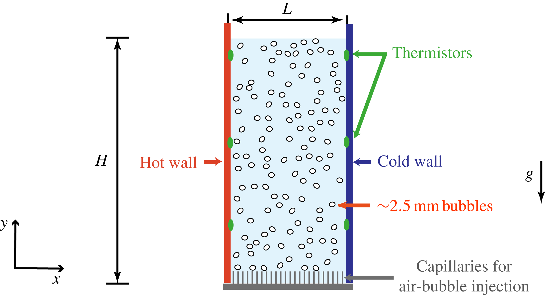
Figure 1. Rectangular bubbly column heated from one side wall and cooled from the other (
 $H=600~\text{mm}$
,
$H=600~\text{mm}$
,
 $L=230~\text{mm}$
). Bubbles of approximately
$L=230~\text{mm}$
). Bubbles of approximately
 $2.5~\text{mm}$
diameter were injected through 180 capillaries placed at the bottom of the set-up (inner diameter
$2.5~\text{mm}$
diameter were injected through 180 capillaries placed at the bottom of the set-up (inner diameter
 $0.21~\text{mm}$
).
$0.21~\text{mm}$
).
As mentioned previously, our set-up resembles one for vertical natural convection since one brass side wall is heated and the other is cooled in order to generate a horizontal temperature gradient in the set-up. More precisely, heating was provided by placing three etched-foil heaters on the outer side of the hot wall. Heaters were connected in parallel to a digitally controlled power supply (Keysight N8741A), providing altogether up to
 $300~\text{W}$
. The other brass wall was cooled by a water circulating bath (PolyTemp PD15R-30). The temperature of the heated and the cooled walls was monitored by three thermistors which were glued at different heights of the cold and warm walls, namely at
$300~\text{W}$
. The other brass wall was cooled by a water circulating bath (PolyTemp PD15R-30). The temperature of the heated and the cooled walls was monitored by three thermistors which were glued at different heights of the cold and warm walls, namely at
 $125~\text{mm}$
,
$125~\text{mm}$
,
 $315~\text{mm}$
and
$315~\text{mm}$
and
 $505~\text{mm}$
. Temperature regulation of both the cold and warm walls was achieved by PID (Proportional-Integral-Derivative) control so that the mean temperature of the walls was maintained constant over time. In order to limit the heat losses, the set-up was wrapped in several layers of insulating blanket and foam. Moreover, an aluminium plate with heaters attached to it was placed on the outer side of the hot wall and maintained at the same temperature as the hot wall to act as a temperature shield.
$505~\text{mm}$
. Temperature regulation of both the cold and warm walls was achieved by PID (Proportional-Integral-Derivative) control so that the mean temperature of the walls was maintained constant over time. In order to limit the heat losses, the set-up was wrapped in several layers of insulating blanket and foam. Moreover, an aluminium plate with heaters attached to it was placed on the outer side of the hot wall and maintained at the same temperature as the hot wall to act as a temperature shield.
Heat losses were estimated to be no more than 7 % by calculating convective heat transport rate from all outer surfaces of the set-up with the assumption that these surfaces are at maximum
 $25^{\circ }\text{C}$
. On the other hand, we measured the power needed to maintain the temperature of the bulk constant (
$25^{\circ }\text{C}$
. On the other hand, we measured the power needed to maintain the temperature of the bulk constant (
 $T_{bulk}=25\,^{\circ }\text{C}$
) over 4 h. Power supplied to the heaters in that way is no more than 3 % of the total power needed when running the actual experiments in which the bulk temperature is also
$T_{bulk}=25\,^{\circ }\text{C}$
) over 4 h. Power supplied to the heaters in that way is no more than 3 % of the total power needed when running the actual experiments in which the bulk temperature is also
 $25^{\circ }$
. We therefore expect the actual heat losses to be in the range of 3 %–7 %, which enables us to study precisely the heat transport driven by a horizontal temperature gradient in a bubbly flow.
$25^{\circ }$
. We therefore expect the actual heat losses to be in the range of 3 %–7 %, which enables us to study precisely the heat transport driven by a horizontal temperature gradient in a bubbly flow.
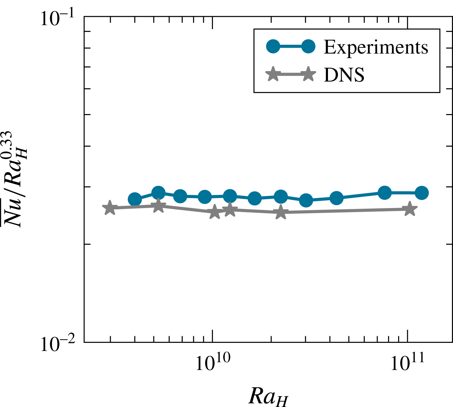
Figure 2. Compensated form of the dependence of Nusselt number
 $\overline{Nu}$
on the Rayleigh number
$\overline{Nu}$
on the Rayleigh number
 $Ra_{H}$
for the single-phase case.
$Ra_{H}$
for the single-phase case.
2.2 Single-phase vertical convection
The single-phase heat transport will be used as a reference for the heat transport enhancement by bubble injection. In a single-phase system a variety of flow regimes can be observed depending on the height
 $H$
, the length
$H$
, the length
 $L$
and the Rayleigh number
$L$
and the Rayleigh number
 $Ra_{H}$
of the system (Bejan Reference Bejan2004). For the parameter range studied here (
$Ra_{H}$
of the system (Bejan Reference Bejan2004). For the parameter range studied here (
 $H/L=2.4$
and
$H/L=2.4$
and
 $Ra_{H}=4.0\times 10^{9}-1.2\times 10^{11}$
) we expect the system to be in a boundary layer dominant regime. In this regime the boundary layers which distinctly form along the heated and cooled side walls control the heat transfer, while the bulk of the fluid is relatively stagnant. Furthermore, previous studies of single-phase vertical convection describe the dependence of Nusselt number on the Rayleigh number in the power law form
$Ra_{H}=4.0\times 10^{9}-1.2\times 10^{11}$
) we expect the system to be in a boundary layer dominant regime. In this regime the boundary layers which distinctly form along the heated and cooled side walls control the heat transfer, while the bulk of the fluid is relatively stagnant. Furthermore, previous studies of single-phase vertical convection describe the dependence of Nusselt number on the Rayleigh number in the power law form
 $Nu\sim Ra^{\unicode[STIX]{x1D6FD}}$
at fixed
$Nu\sim Ra^{\unicode[STIX]{x1D6FD}}$
at fixed
 $Pr$
, with exponent
$Pr$
, with exponent
 $\unicode[STIX]{x1D6FD}$
ranging between
$\unicode[STIX]{x1D6FD}$
ranging between
 $1/4$
and
$1/4$
and
 $1/3$
(see Ng et al. (Reference Ng, Ooi, Lohse and Chung2015, Reference Ng, Ooi, Lohse and Chung2017) and references within). We find that for the range of
$1/3$
(see Ng et al. (Reference Ng, Ooi, Lohse and Chung2015, Reference Ng, Ooi, Lohse and Chung2017) and references within). We find that for the range of
 $Ra_{H}$
studied here the effective scaling exponent is
$Ra_{H}$
studied here the effective scaling exponent is
 $\unicode[STIX]{x1D6FD}\approx 0.33\pm 0.02$
, which lies within the expected range as can be seen in the compensated plot in figure 2.
$\unicode[STIX]{x1D6FD}\approx 0.33\pm 0.02$
, which lies within the expected range as can be seen in the compensated plot in figure 2.
For the single-phase flow we benchmark the heat transfer against direct numerical simulations (DNS). For this purpose an in-house second-order finite difference code (van der Poel et al.
Reference van der Poel, Ostilla-Mónico, Donners and Verzicco2015; Zhu et al.
Reference Zhu, Phillips, Spandan, Donners, Ruetsch, Romero, Ostilla-Mónico, Yang, Lohse and Verzicco2018) was used to solve the three-dimensional Boussinesq equations for the single-phase vertical convection. The code has been extensively validated and used for Rayleigh–Bénard flow (van der Poel et al.
Reference van der Poel, Ostilla-Mónico, Donners and Verzicco2015; Zhu et al.
Reference Zhu, Phillips, Spandan, Donners, Ruetsch, Romero, Ostilla-Mónico, Yang, Lohse and Verzicco2018), in which the only difference is the direction of the buoyancy force. The computational box has the same size as has been employed in the experiments. The no-slip boundary conditions are adopted for the velocity at all solid boundaries. At the top and bottom walls, the heat insulating conditions are employed, and at the left and right plates, constant temperatures are prescribed. The resolution of the simulations is fine enough to guarantee that the results are grid-independent. Figure 2 shows good agreement between numerical and experimental results, within the range of uncertainty. As the experimental set-up was not completely insulated at the top and due to unavoidable heat losses to the outside, the experimentally obtained
 $\overline{Nu}$
are slightly higher.
$\overline{Nu}$
are slightly higher.
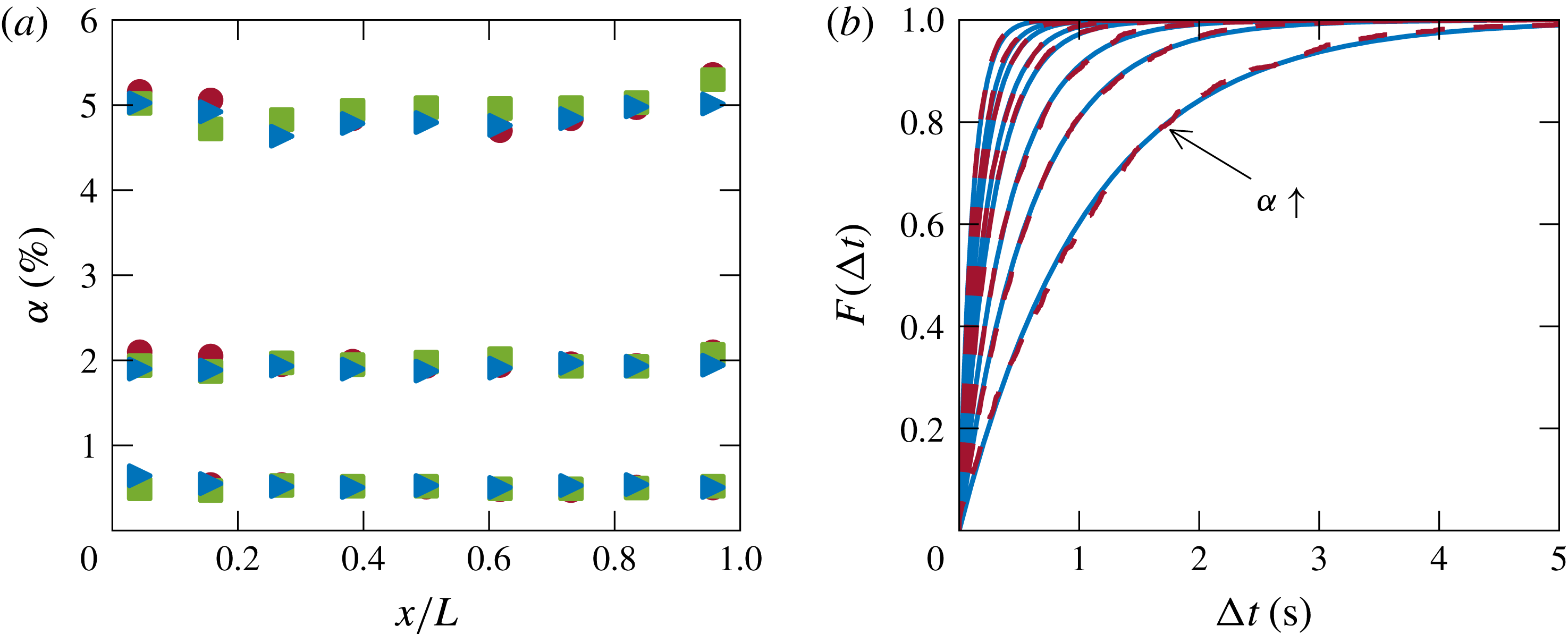
Figure 3. (a) Gas volume fraction
 $\unicode[STIX]{x1D6FC}$
at different measurement positions in the experimental set-up: ▸,
$\unicode[STIX]{x1D6FC}$
at different measurement positions in the experimental set-up: ▸,
 $H=125~\text{mm}$
; ▪,
$H=125~\text{mm}$
; ▪,
 $H=315~\text{mm}$
; ●,
$H=315~\text{mm}$
; ●,
 $H=505~\text{mm}$
. (b) Cumulative distribution function of the time interval between consecutive bubbles in the centre of the set-up for
$H=505~\text{mm}$
. (b) Cumulative distribution function of the time interval between consecutive bubbles in the centre of the set-up for
 $\unicode[STIX]{x1D6FC}=0.3\,\%$
,
$\unicode[STIX]{x1D6FC}=0.3\,\%$
,
 $0.5\,\%$
,
$0.5\,\%$
,
 $0.9\,\%$
,
$0.9\,\%$
,
 $1.5\,\%$
,
$1.5\,\%$
,
 $2\,\%$
,
$2\,\%$
,
 $3.0\,\%$
,
$3.0\,\%$
,
 $3.9\,\%$
and
$3.9\,\%$
and
 $6.0\,\%$
, respectively. Solid lines represent experimental measurements while dashed lines represent Poisson’s process.
$6.0\,\%$
, respectively. Solid lines represent experimental measurements while dashed lines represent Poisson’s process.
2.3 Instrumentation for the gas phase characterisation
The homogeneity of the bubble swarm was verified by measuring the gas volume fraction
 $\unicode[STIX]{x1D6FC}$
at different locations within the flow by means of a single optical fibre probe. In the absence of a temperature gradient, we observe that
$\unicode[STIX]{x1D6FC}$
at different locations within the flow by means of a single optical fibre probe. In the absence of a temperature gradient, we observe that
 $\unicode[STIX]{x1D6FC}$
is nearly uniform along the length
$\unicode[STIX]{x1D6FC}$
is nearly uniform along the length
 $L$
and height
$L$
and height
 $H$
of the set-up (see figure 3
a). We also note that no large-scale clustering is present, since the cumulative distribution function
$H$
of the set-up (see figure 3
a). We also note that no large-scale clustering is present, since the cumulative distribution function
 $F(\unicode[STIX]{x0394}t)$
of the time between consecutive bubbles
$F(\unicode[STIX]{x0394}t)$
of the time between consecutive bubbles
 $\unicode[STIX]{x0394}t$
is Poissonian (see figure 3
b and Risso & Ellingsen (Reference Risso and Ellingsen2002) for more details). In the presence of heating, the homogeneity of the swarm was comparable to that without heating, with no more than 2 % variation. The bubble swarm thus remained homogeneous even with heating, indicating that the bubbly flow was not destabilised by the temperature gradient. We further characterised the gas phase by measuring the bubble diameter and the bubble rising velocity with an in-house dual optical fibre probe (Alméras et al.
Reference Alméras, Mathai, Lohse and Sun2017). Bubble diameter
$\unicode[STIX]{x0394}t$
is Poissonian (see figure 3
b and Risso & Ellingsen (Reference Risso and Ellingsen2002) for more details). In the presence of heating, the homogeneity of the swarm was comparable to that without heating, with no more than 2 % variation. The bubble swarm thus remained homogeneous even with heating, indicating that the bubbly flow was not destabilised by the temperature gradient. We further characterised the gas phase by measuring the bubble diameter and the bubble rising velocity with an in-house dual optical fibre probe (Alméras et al.
Reference Alméras, Mathai, Lohse and Sun2017). Bubble diameter
 $d_{eq}$
and bubble rise velocity
$d_{eq}$
and bubble rise velocity
 $V_{b}$
lie in the ranges
$V_{b}$
lie in the ranges
 $[2.1,~3.4]~\text{mm}$
and
$[2.1,~3.4]~\text{mm}$
and
 $[0.24,~0.34]~\text{m}~\text{s}^{-1}$
, respectively (see figure 4
a,b), resulting in a bubble Reynolds number
$[0.24,~0.34]~\text{m}~\text{s}^{-1}$
, respectively (see figure 4
a,b), resulting in a bubble Reynolds number
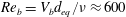 $Re_{b}=V_{b}d_{eq}/\unicode[STIX]{x1D708}\approx 600$
. The bubble rise velocity follows the same trend as previously observed by Riboux et al. (Reference Riboux, Risso and Legendre2010), namely it evolves roughly as
$Re_{b}=V_{b}d_{eq}/\unicode[STIX]{x1D708}\approx 600$
. The bubble rise velocity follows the same trend as previously observed by Riboux et al. (Reference Riboux, Risso and Legendre2010), namely it evolves roughly as
 $V_{bub}\propto \unicode[STIX]{x1D6FC}^{-0.1}$
. These values of bubble diameter (respectively bubble velocities) fall within the expected range for this configuration of needle injection (respectively bubble diameter). Once compared to those found by Riboux et al. (Reference Riboux, Risso and Legendre2010) and Alméras (Reference Alméras2014), we find up to 6 % variation, which is acceptable since it can be attributed to slightly different bubble injection section and water quality.
$V_{bub}\propto \unicode[STIX]{x1D6FC}^{-0.1}$
. These values of bubble diameter (respectively bubble velocities) fall within the expected range for this configuration of needle injection (respectively bubble diameter). Once compared to those found by Riboux et al. (Reference Riboux, Risso and Legendre2010) and Alméras (Reference Alméras2014), we find up to 6 % variation, which is acceptable since it can be attributed to slightly different bubble injection section and water quality.
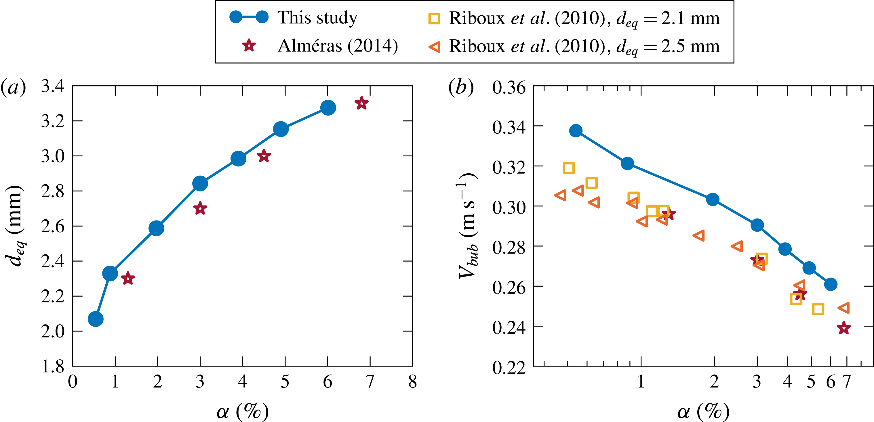
Figure 4. (a) Mean bubble diameter
 $d_{eq}$
and (b) bubble rise velocity
$d_{eq}$
and (b) bubble rise velocity
 $V_{bub}$
for the studied gas volume fractions
$V_{bub}$
for the studied gas volume fractions
 $\unicode[STIX]{x1D6FC}$
, in comparison to different experimental studies.
$\unicode[STIX]{x1D6FC}$
, in comparison to different experimental studies.
2.4 Instrumentation for the heat flux and temperature measurements
In the present study, we performed global and local characterisations of the heat transfer. In order to obtain
 $\overline{Nu}$
and
$\overline{Nu}$
and
 $Ra_{H}$
, we measured the hot and cold wall temperatures, and the heat input to the system
$Ra_{H}$
, we measured the hot and cold wall temperatures, and the heat input to the system
 $Q$
. To this end, resistances of the thermistors placed on the hot and cold walls were read out every 4.2 s using a digital multimeter (Keysight 34970A). The temperature is then converted from the resistances based on the calibrations of the individual thermistors. The total heater power input was measured as
$Q$
. To this end, resistances of the thermistors placed on the hot and cold walls were read out every 4.2 s using a digital multimeter (Keysight 34970A). The temperature is then converted from the resistances based on the calibrations of the individual thermistors. The total heater power input was measured as
 $Q=\sum Q_{i}=Q_{i}=I_{i}\cdot V_{i}$
, where
$Q=\sum Q_{i}=Q_{i}=I_{i}\cdot V_{i}$
, where
 $I_{i}$
and
$I_{i}$
and
 $V_{i}$
are the current and voltage across each heater, respectively. The experimental measurements were performed after steady state was achieved in which the mean wall temperatures fluctuated less than
$V_{i}$
are the current and voltage across each heater, respectively. The experimental measurements were performed after steady state was achieved in which the mean wall temperatures fluctuated less than
 $\pm ~0.01\text{K}$
(respectively
$\pm ~0.01\text{K}$
(respectively
 $\pm 0.1~\text{K}$
) for the lowest
$\pm 0.1~\text{K}$
) for the lowest
 $Ra_{H}$
and
$Ra_{H}$
and
 $\pm 0.4~\text{K}$
(respectively
$\pm 0.4~\text{K}$
(respectively
 $\pm 0.5~\text{K}$
) for the highest
$\pm 0.5~\text{K}$
) for the highest
 $Ra_{H}$
, for the single-phase (respectively two-phase) case. Time averaging of the instantaneous power supplied to each heater
$Ra_{H}$
, for the single-phase (respectively two-phase) case. Time averaging of the instantaneous power supplied to each heater
 $Q_{i}$
was then performed over a total time period of 6 h for single-phase cases, and 3 h for two-phase cases.
$Q_{i}$
was then performed over a total time period of 6 h for single-phase cases, and 3 h for two-phase cases.
For a better understanding of the heat transfer, we performed local measurements of the liquid temperature fluctuations:
 $T^{\prime }=T-\langle T\rangle$
, where
$T^{\prime }=T-\langle T\rangle$
, where
 $T^{\prime }$
denotes the temperature fluctuations,
$T^{\prime }$
denotes the temperature fluctuations,
 $T$
the measured instantaneous temperature and
$T$
the measured instantaneous temperature and
 $\langle T\rangle$
the time-averaged temperature at the measurement point. For each operating condition, temperature fluctuations were recorded for at least 180 min (respectively 360 min) in the two-phase (respectively single-phase) case once the flow was stable, which yields satisfactory statistical convergence. We used a negative temperature coefficient (NTC) miniature thermistor manufactured by TE connectivity (Measurement Specialties G22K7MCD419) with a tip diameter of
$\langle T\rangle$
the time-averaged temperature at the measurement point. For each operating condition, temperature fluctuations were recorded for at least 180 min (respectively 360 min) in the two-phase (respectively single-phase) case once the flow was stable, which yields satisfactory statistical convergence. We used a negative temperature coefficient (NTC) miniature thermistor manufactured by TE connectivity (Measurement Specialties G22K7MCD419) with a tip diameter of
 $0.38~\text{mm}$
, and a response time of
$0.38~\text{mm}$
, and a response time of
 $30~\text{ms}$
in water. The thermistor was connected as one arm of a Wheatstone bridge so that very small variations of the thermistors’ resistance could be measured. For noise reduction we used a Lock-In amplifier (SR830). The function of the Lock-In amplifier is to firstly supply voltage to the bridge and then filter out noise at frequencies which are different from that of the signal range. This ensured milli-Kelvin resolution of the temperature fluctuations. In order to measure the temperature with this resolution reliably, the thermistors were calibrated in a circulating bath with
$30~\text{ms}$
in water. The thermistor was connected as one arm of a Wheatstone bridge so that very small variations of the thermistors’ resistance could be measured. For noise reduction we used a Lock-In amplifier (SR830). The function of the Lock-In amplifier is to firstly supply voltage to the bridge and then filter out noise at frequencies which are different from that of the signal range. This ensured milli-Kelvin resolution of the temperature fluctuations. In order to measure the temperature with this resolution reliably, the thermistors were calibrated in a circulating bath with
 $5~\text{mK}$
stability. A typical obtained signals in single-phase and two-phase are presented in figure 5(a,b), respectively. It is interesting to note that the temperature fluctuations are up to 200 times stronger in the two-phase case and this will be discussed in § 4.
$5~\text{mK}$
stability. A typical obtained signals in single-phase and two-phase are presented in figure 5(a,b), respectively. It is interesting to note that the temperature fluctuations are up to 200 times stronger in the two-phase case and this will be discussed in § 4.
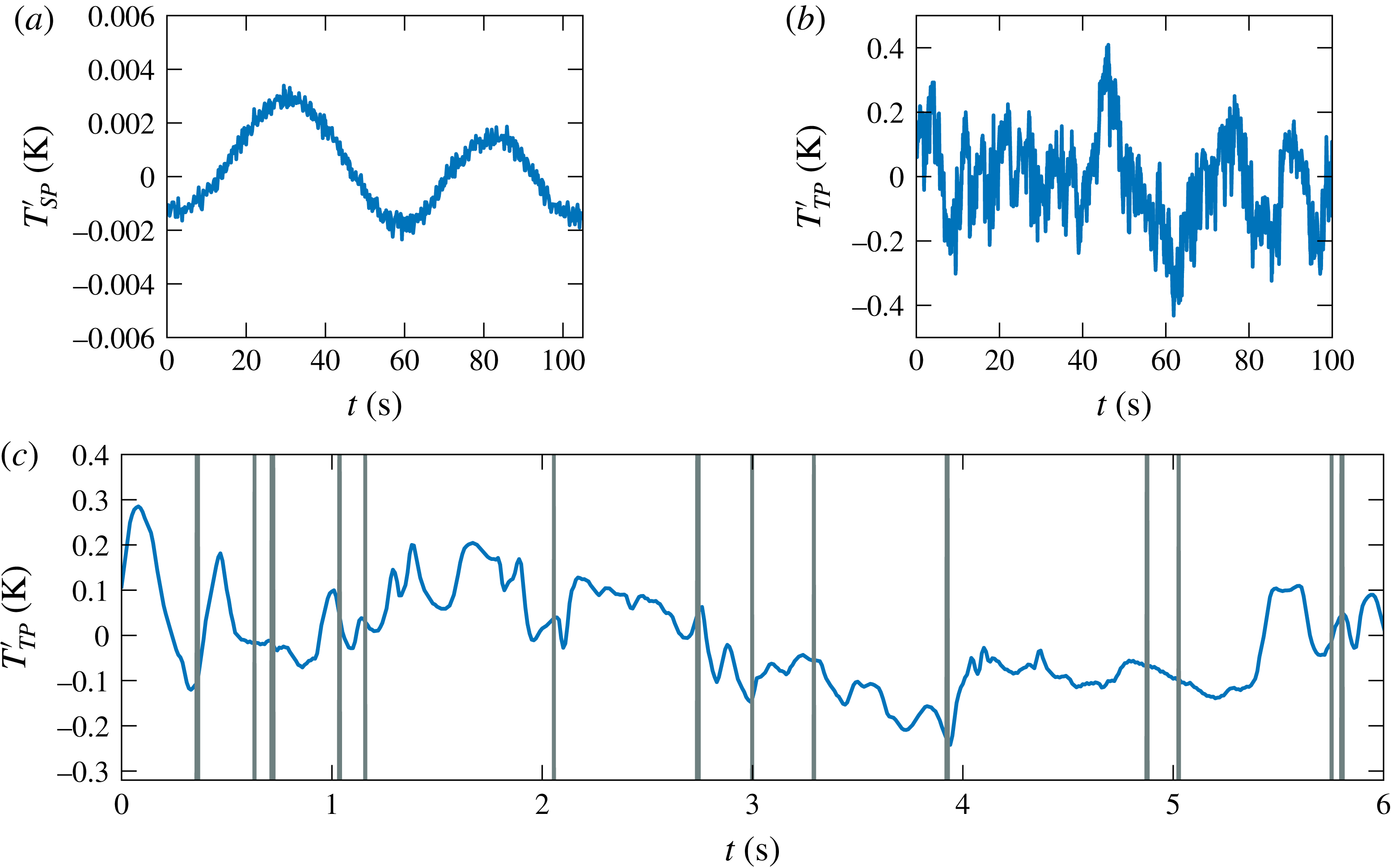
Figure 5. Signal of the temperature fluctuations at
 $L=11.5~\text{cm}$
for
$L=11.5~\text{cm}$
for
 $Ra_{H}=2.2\times 10^{10}$
in (a) single-phase flow
$Ra_{H}=2.2\times 10^{10}$
in (a) single-phase flow
 $T_{SP}^{\prime }$
(observed frequency of approximately
$T_{SP}^{\prime }$
(observed frequency of approximately
 $10^{-2}~\text{Hz}$
corresponds to large-scale circulation frequency, which is addressed in § 4), (b) two-phase flow
$10^{-2}~\text{Hz}$
corresponds to large-scale circulation frequency, which is addressed in § 4), (b) two-phase flow
 $\unicode[STIX]{x1D6FC}=0.9\,\%$
 $T_{TP}^{\prime }$
, and (c) enlarged simultaneously obtained temperature fluctuations and optical fibre signal where each grey vertical line is a passage of a single bubble.
$T_{TP}^{\prime }$
, and (c) enlarged simultaneously obtained temperature fluctuations and optical fibre signal where each grey vertical line is a passage of a single bubble.
The local temperature measurement technique used here is well established for single-phase flow (Belmonte, Tilgner & Libchaber Reference Belmonte, Tilgner and Libchaber1994); however, until now it has never been used for temperature fluctuation measurements in bubbly flows. Since the presence of bubbles may perturb the local measurements by interacting directly with the probe (Rensen et al.
Reference Rensen, Luther and Lohse2005; Mercado Martínez et al.
Reference Mercado Martínez, Chehata Gǿmez, Van Gils, Sun and Lohse2010), it is necessary to validate the technique for two-phase flow. For this purpose we made an in-house probe in which an optical fibre and the thermistor were positioned
 ${\sim}1~\text{mm}$
apart in the horizontal plane and with the thermistor placed
${\sim}1~\text{mm}$
apart in the horizontal plane and with the thermistor placed
 ${\sim}1~\text{mm}$
below the fibre tip. Figure 5(c) shows typical thermistor (blue line) and optical fibre (vertical grey lines) signals simultaneously obtained. The optical fibre allows us to detect the presence of the bubble at the probe tip; it was thus possible to remove parts of the temperature signal corresponding to bubble–probe collisions (Mercado Martínez et al.
Reference Mercado Martínez, Chehata Gǿmez, Van Gils, Sun and Lohse2010), and to compare the statistical properties of this truncated temperature signal with the original signal. The difference in the statistics (mean, standard deviation, kurtosis, skewness) obtained from the original and the truncated signal was minor (
${\sim}1~\text{mm}$
below the fibre tip. Figure 5(c) shows typical thermistor (blue line) and optical fibre (vertical grey lines) signals simultaneously obtained. The optical fibre allows us to detect the presence of the bubble at the probe tip; it was thus possible to remove parts of the temperature signal corresponding to bubble–probe collisions (Mercado Martínez et al.
Reference Mercado Martínez, Chehata Gǿmez, Van Gils, Sun and Lohse2010), and to compare the statistical properties of this truncated temperature signal with the original signal. The difference in the statistics (mean, standard deviation, kurtosis, skewness) obtained from the original and the truncated signal was minor (
 ${\approx}0.05\,\%$
). This suggests that the short durations of the bubble–thermistor contact (
${\approx}0.05\,\%$
). This suggests that the short durations of the bubble–thermistor contact (
 $t_{int}=d_{eq}/V_{bub}=7.2~\text{ms}$
for
$t_{int}=d_{eq}/V_{bub}=7.2~\text{ms}$
for
 $\unicode[STIX]{x1D6FC}=0.9\,\%$
) were filtered out due to the longer response time of the thermistor (
$\unicode[STIX]{x1D6FC}=0.9\,\%$
) were filtered out due to the longer response time of the thermistor (
 $t_{r}\sim 30~\text{ms}$
). Nevertheless, the thermistor response time is sufficiently short to measure the temperature fluctuations between two bubble passages. From table 1 we see that
$t_{r}\sim 30~\text{ms}$
). Nevertheless, the thermistor response time is sufficiently short to measure the temperature fluctuations between two bubble passages. From table 1 we see that
 $t_{2b}$
is sufficiently long when compared to
$t_{2b}$
is sufficiently long when compared to
 $t_{r}$
even for higher gas volume fractions. Furthermore, the estimated time of the bubble–thermistor contact remains much shorter than
$t_{r}$
even for higher gas volume fractions. Furthermore, the estimated time of the bubble–thermistor contact remains much shorter than
 $t_{r}$
for
$t_{r}$
for
 $\unicode[STIX]{x1D6FC}$
up to
$\unicode[STIX]{x1D6FC}$
up to
 $5\,\%$
(see table 1). The present measurement technique is thus suitable for measurements of the temperature fluctuations in the liquid phase not only for
$5\,\%$
(see table 1). The present measurement technique is thus suitable for measurements of the temperature fluctuations in the liquid phase not only for
 $\unicode[STIX]{x1D6FC}=0.9\,\%$
, but also for higher gas volume fractions.
$\unicode[STIX]{x1D6FC}=0.9\,\%$
, but also for higher gas volume fractions.
Table 1. Measured mean time between bubble passages
 $t_{2b}$
and estimated time of bubble–thermistor contact
$t_{2b}$
and estimated time of bubble–thermistor contact
 $t_{int}$
for the studied gas volume fractions
$t_{int}$
for the studied gas volume fractions
 $\unicode[STIX]{x1D6FC}$
.
$\unicode[STIX]{x1D6FC}$
.
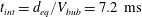
3 Global heat transport enhancement
Let us now discuss the heat transport in the presence of a homogeneous bubble swarm for gas volume fraction
 $\unicode[STIX]{x1D6FC}$
ranging from 0.5 % to 5 %, and the Rayleigh number ranging from
$\unicode[STIX]{x1D6FC}$
ranging from 0.5 % to 5 %, and the Rayleigh number ranging from
 $4.0\times 10^{9}$
to at most
$4.0\times 10^{9}$
to at most
 $3.6\times 10^{10}$
(see figure 6). For the whole range of
$3.6\times 10^{10}$
(see figure 6). For the whole range of
 $\unicode[STIX]{x1D6FC}$
and
$\unicode[STIX]{x1D6FC}$
and
 $Ra_{H}$
, adding bubbles considerably increases the heat transport, since the Nusselt number is approximately an order of magnitude higher as compared to single-phase flow (see figure 6
a). In order to better quantify the heat transport enhancement due to bubble injection, we show in figure 6(b) the ratio of the Nusselt number in the bubbly flow
$Ra_{H}$
, adding bubbles considerably increases the heat transport, since the Nusselt number is approximately an order of magnitude higher as compared to single-phase flow (see figure 6
a). In order to better quantify the heat transport enhancement due to bubble injection, we show in figure 6(b) the ratio of the Nusselt number in the bubbly flow
 $\overline{Nu_{b}}$
to the Nusselt number in the single-phase
$\overline{Nu_{b}}$
to the Nusselt number in the single-phase
 $\overline{Nu_{0}}$
as a function of
$\overline{Nu_{0}}$
as a function of
 $Ra_{H}$
for different
$Ra_{H}$
for different
 $\unicode[STIX]{x1D6FC}$
. We find that heat transfer is enhanced up to 20 times due to bubble injection, and that the enhancement increases with increasing
$\unicode[STIX]{x1D6FC}$
. We find that heat transfer is enhanced up to 20 times due to bubble injection, and that the enhancement increases with increasing
 $\unicode[STIX]{x1D6FC}$
and decreasing
$\unicode[STIX]{x1D6FC}$
and decreasing
 $Ra_{H}$
. Note that the decreasing trend of
$Ra_{H}$
. Note that the decreasing trend of
 $\overline{Nu_{b}}/\overline{Nu_{0}}$
with
$\overline{Nu_{b}}/\overline{Nu_{0}}$
with
 $Ra_{H}$
occurs because the single-phase heat flux
$Ra_{H}$
occurs because the single-phase heat flux
 $\overline{Nu_{0}}$
increases with
$\overline{Nu_{0}}$
increases with
 $Ra_{H}$
.
$Ra_{H}$
.
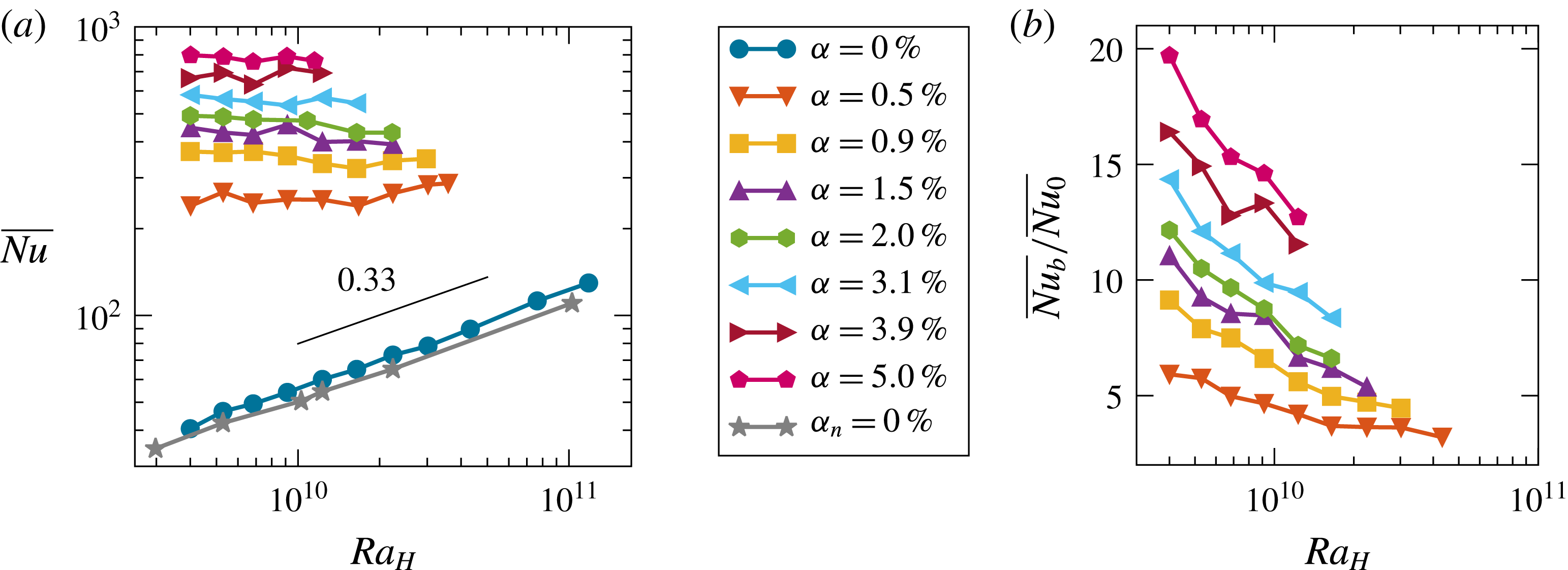
Figure 6. (a) Dependence of Nusselt number
 $\overline{Nu}$
on the Rayleigh
$\overline{Nu}$
on the Rayleigh
 $Ra_{H}$
number for different gas volume fractions (
$Ra_{H}$
number for different gas volume fractions (
 $\unicode[STIX]{x1D6FC}$
, experimental data;
$\unicode[STIX]{x1D6FC}$
, experimental data;
 $\unicode[STIX]{x1D6FC}_{n}$
, numerical simulations); the size of the symbol corresponds to the error bar. (b) Heat transfer enhancement:
$\unicode[STIX]{x1D6FC}_{n}$
, numerical simulations); the size of the symbol corresponds to the error bar. (b) Heat transfer enhancement:
 $\overline{Nu}_{0}$
, Nusselt number in single-phase case;
$\overline{Nu}_{0}$
, Nusselt number in single-phase case;
 $\overline{Nu}_{b}$
, Nusselt number in bubbly flow.
$\overline{Nu}_{b}$
, Nusselt number in bubbly flow.
Figure 7. The profile of the gas volume fraction for
 $\unicode[STIX]{x1D6FC}=0.9\,\%$
at half-height for different imposed temperature differences between hot and cold wall
$\unicode[STIX]{x1D6FC}=0.9\,\%$
at half-height for different imposed temperature differences between hot and cold wall
 $\unicode[STIX]{x0394}T$
.
$\unicode[STIX]{x0394}T$
.
Figure 6(a) also shows that for a fixed
 $\unicode[STIX]{x1D6FC}\geqslant 0.5\,\%$
 $\overline{Nu}$
remains nearly constant with increasing
$\overline{Nu}$
remains nearly constant with increasing
 $Ra_{H}$
. This indicates that the boundary layers developing along the walls are no longer limiting the heat transport in the two-phase case. Together with the observation that the heating does not induce a gradient in the gas volume fraction profile (see figure 7), this further implies that the temperature behaves as a passive scalar in bubbly flow. In order to understand the mechanism of the heat transport in bubbly flow we compare the findings of our study to those of Alméras et al. (Reference Alméras, Risso, Roig, Cazin, Plais and Augier2015), who showed that the transport of a passive scalar at high Péclet number (
$Ra_{H}$
. This indicates that the boundary layers developing along the walls are no longer limiting the heat transport in the two-phase case. Together with the observation that the heating does not induce a gradient in the gas volume fraction profile (see figure 7), this further implies that the temperature behaves as a passive scalar in bubbly flow. In order to understand the mechanism of the heat transport in bubbly flow we compare the findings of our study to those of Alméras et al. (Reference Alméras, Risso, Roig, Cazin, Plais and Augier2015), who showed that the transport of a passive scalar at high Péclet number (
 $Pe=V_{bub}d_{eq}/D\approx 10^{6}$
, with
$Pe=V_{bub}d_{eq}/D\approx 10^{6}$
, with
 $V_{bub}$
as the bubble velocity and
$V_{bub}$
as the bubble velocity and
 $d_{eq}$
as the bubble diameter and
$d_{eq}$
as the bubble diameter and
 $D$
as molecular diffusivity) by a homogeneous bubble swarm is a diffusive process. In the case of a diffusive process, the turbulent heat flux can be modelled as
$D$
as molecular diffusivity) by a homogeneous bubble swarm is a diffusive process. In the case of a diffusive process, the turbulent heat flux can be modelled as
 $\overline{u_{i}^{\prime }T^{\prime }}=-D_{ii}\unicode[STIX]{x1D735}\overline{T}$
, introducing the effective diffusivity
$\overline{u_{i}^{\prime }T^{\prime }}=-D_{ii}\unicode[STIX]{x1D735}\overline{T}$
, introducing the effective diffusivity
 $D_{ii}$
. If we take the heat transport to be a diffusive process in our study, the Nusselt number can be interpreted as the ratio between the effective diffusivity induced by the bubble swarm
$D_{ii}$
. If we take the heat transport to be a diffusive process in our study, the Nusselt number can be interpreted as the ratio between the effective diffusivity induced by the bubble swarm
 $D_{ii}$
and the thermal diffusivity
$D_{ii}$
and the thermal diffusivity
 $\unicode[STIX]{x1D712}$
. Thus, from our measurements we can estimate the effective diffusivity induced by a bubble swarm for a gas volume fraction ranging from 0.5 % to 5 %. Note that since the temperature gradient is imposed in the horizontal direction, we assume that the measured effective diffusivity is mainly in the horizontal direction. Figure 8(a) shows the Nusselt number
$\unicode[STIX]{x1D712}$
. Thus, from our measurements we can estimate the effective diffusivity induced by a bubble swarm for a gas volume fraction ranging from 0.5 % to 5 %. Note that since the temperature gradient is imposed in the horizontal direction, we assume that the measured effective diffusivity is mainly in the horizontal direction. Figure 8(a) shows the Nusselt number
 $\langle \overline{Nu}\rangle$
averaged over the full range of Rayleigh number for a constant gas volume fraction as a function of
$\langle \overline{Nu}\rangle$
averaged over the full range of Rayleigh number for a constant gas volume fraction as a function of
 $\unicode[STIX]{x1D6FC}$
. We clearly see that the averaged Nusselt number evolves as
$\unicode[STIX]{x1D6FC}$
. We clearly see that the averaged Nusselt number evolves as
 $\unicode[STIX]{x1D6FC}^{0.45\pm 0.025}$
. Even if we subtract the single-phase Nusselt number (which might be thought of as the contribution of natural convection to the total heat transfer) from the one in bubbly flow, the scaling remains unchanged (see figure 8
b). This trend is in good agreement with the model of effective diffusivity proposed by Alméras et al. (Reference Alméras, Risso, Roig, Cazin, Plais and Augier2015). In fact, the authors showed that at low gas volume fraction, the diffusion coefficient can be written as
$\unicode[STIX]{x1D6FC}^{0.45\pm 0.025}$
. Even if we subtract the single-phase Nusselt number (which might be thought of as the contribution of natural convection to the total heat transfer) from the one in bubbly flow, the scaling remains unchanged (see figure 8
b). This trend is in good agreement with the model of effective diffusivity proposed by Alméras et al. (Reference Alméras, Risso, Roig, Cazin, Plais and Augier2015). In fact, the authors showed that at low gas volume fraction, the diffusion coefficient can be written as
 $D_{ii}\propto u^{\prime }\unicode[STIX]{x1D6EC}$
, where
$D_{ii}\propto u^{\prime }\unicode[STIX]{x1D6EC}$
, where
 $u^{\prime }$
is the standard deviation of the velocity fluctuations, and
$u^{\prime }$
is the standard deviation of the velocity fluctuations, and
 $\unicode[STIX]{x1D6EC}$
is the integral Lagrangian length scale (
$\unicode[STIX]{x1D6EC}$
is the integral Lagrangian length scale (
 $\unicode[STIX]{x1D6EC}\simeq d_{bub}/C_{d0}$
,
$\unicode[STIX]{x1D6EC}\simeq d_{bub}/C_{d0}$
,
 $C_{d0}=4d_{bub}g/3{V_{0}}^{2}$
, here
$C_{d0}=4d_{bub}g/3{V_{0}}^{2}$
, here
 $C_{d0}$
is the drag coefficient and
$C_{d0}$
is the drag coefficient and
 $V_{0}$
is the rise velocity of a single bubble (Riboux et al.
Reference Riboux, Risso and Legendre2010)). In the expression for the diffusion coefficient only
$V_{0}$
is the rise velocity of a single bubble (Riboux et al.
Reference Riboux, Risso and Legendre2010)). In the expression for the diffusion coefficient only
 $u^{\prime }$
depends on the gas volume fraction and this dependence is given by
$u^{\prime }$
depends on the gas volume fraction and this dependence is given by
 $u^{\prime }\sim V_{0}\unicode[STIX]{x1D6FC}^{0.4}$
(Risso & Ellingsen Reference Risso and Ellingsen2002). In the present study, we expect to have a similar liquid agitation since bubble rising velocity and diameter are comparable. This yields the same evolution of the effective diffusivity
$u^{\prime }\sim V_{0}\unicode[STIX]{x1D6FC}^{0.4}$
(Risso & Ellingsen Reference Risso and Ellingsen2002). In the present study, we expect to have a similar liquid agitation since bubble rising velocity and diameter are comparable. This yields the same evolution of the effective diffusivity
 $D_{ii}$
with the gas volume fraction
$D_{ii}$
with the gas volume fraction
 $\unicode[STIX]{x1D6FC}$
, namely
$\unicode[STIX]{x1D6FC}$
, namely
 $D_{ii}\propto \unicode[STIX]{x1D6FC}^{0.45}$
, extending the model proposed by Alméras et al. (Reference Alméras, Risso, Roig, Cazin, Plais and Augier2015) to lower Péclet numbers (
$D_{ii}\propto \unicode[STIX]{x1D6FC}^{0.45}$
, extending the model proposed by Alméras et al. (Reference Alméras, Risso, Roig, Cazin, Plais and Augier2015) to lower Péclet numbers (
 $Pe\approx 5000$
in this study). We must also stress here that the influence of the Péclet number on the effective diffusivity can be significant. In fact, a numerical simulation performed by Loisy (Reference Loisy2016), at
$Pe\approx 5000$
in this study). We must also stress here that the influence of the Péclet number on the effective diffusivity can be significant. In fact, a numerical simulation performed by Loisy (Reference Loisy2016), at
 $\unicode[STIX]{x1D6FC}=2.4\,\%$
and
$\unicode[STIX]{x1D6FC}=2.4\,\%$
and
 $Re_{b}=30$
, shows that the effective diffusivity normalised by the molecular/thermal diffusivity varies linearly with the Péclet number (for
$Re_{b}=30$
, shows that the effective diffusivity normalised by the molecular/thermal diffusivity varies linearly with the Péclet number (for
 $Pe$
ranging from
$Pe$
ranging from
 $10^{3}$
to
$10^{3}$
to
 $10^{6}$
). Consequently, since the Péclet number varies by three decades between the present study and that of Alméras et al. (Reference Alméras, Risso, Roig, Cazin, Plais and Augier2015), no quantitative comparison of the effective diffusivity can be performed. Therefore, further studies of the effect of the Péclet number on the effective diffusivity at high Reynolds number should be performed.
$10^{6}$
). Consequently, since the Péclet number varies by three decades between the present study and that of Alméras et al. (Reference Alméras, Risso, Roig, Cazin, Plais and Augier2015), no quantitative comparison of the effective diffusivity can be performed. Therefore, further studies of the effect of the Péclet number on the effective diffusivity at high Reynolds number should be performed.
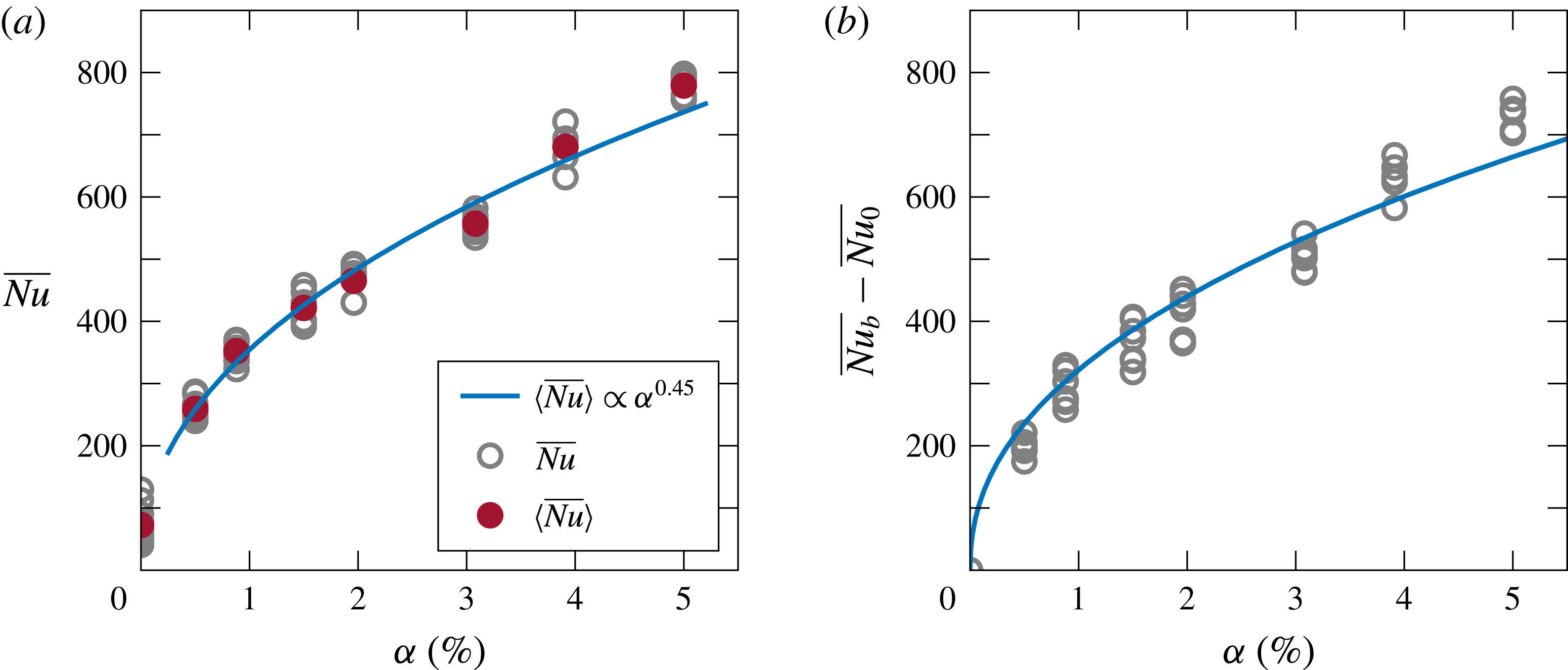
Figure 8. (a) Dependence of Nusselt number
 $\overline{Nu}$
on gas volume fraction
$\overline{Nu}$
on gas volume fraction
 $\unicode[STIX]{x1D6FC}$
(open grey circles represent all the experimental measurements; filled red circles are values of Nusselt number averaged over the studied range of
$\unicode[STIX]{x1D6FC}$
(open grey circles represent all the experimental measurements; filled red circles are values of Nusselt number averaged over the studied range of
 $Ra_{H}$
for each gas volume fraction). (b) The scaling of the difference between the Nusselt number in bubbly flow
$Ra_{H}$
for each gas volume fraction). (b) The scaling of the difference between the Nusselt number in bubbly flow
 $\overline{Nu}_{b}$
and the Nusselt number in single-phase case
$\overline{Nu}_{b}$
and the Nusselt number in single-phase case
 $\overline{Nu}_{0}$
as a function of
$\overline{Nu}_{0}$
as a function of
 $\unicode[STIX]{x1D6FC}$
; the blue curve corresponds to
$\unicode[STIX]{x1D6FC}$
; the blue curve corresponds to
 $\overline{Nu_{b}}-\overline{Nu_{0}}\propto \unicode[STIX]{x1D6FC}^{0.45}$
.
$\overline{Nu_{b}}-\overline{Nu_{0}}\propto \unicode[STIX]{x1D6FC}^{0.45}$
.
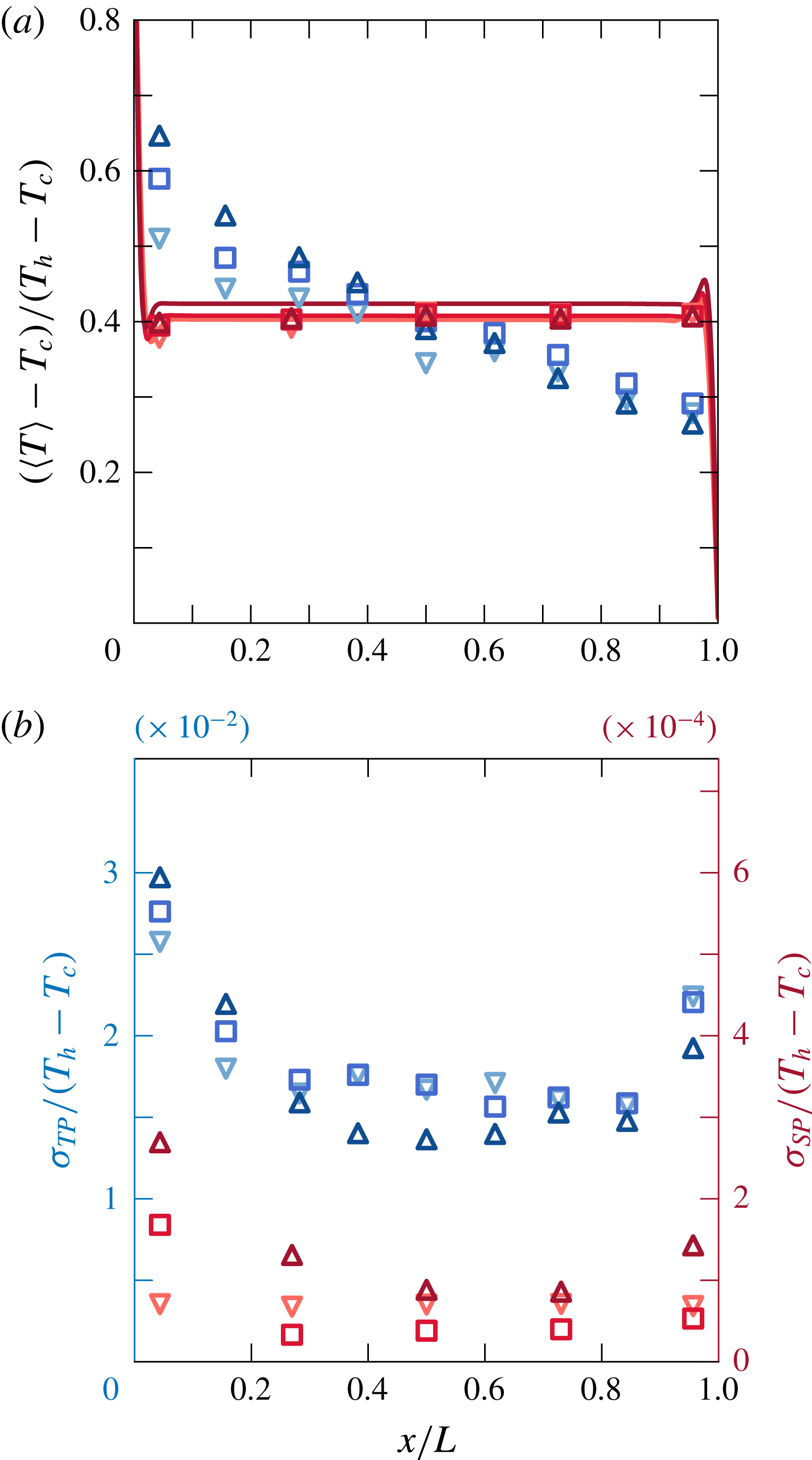
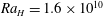
Figure 9. (a) Normalised mean temperature profile at the mid-height. The overshoots close to the walls in the numerical data appear because the thin layer of warmed up (cooled down) fluids moving upward (downward) are still colder (hotter) than the bulk where there is a stable stratification. (b) Normalised standard deviation of the temperature fluctuations. Red lines (numerical results in a) and symbols (experimental data) represent the single-phase case and blue symbols the two-phase case with
 $\unicode[STIX]{x1D6FC}=0.9\,\%$
, for various Rayleigh numbers:
$\unicode[STIX]{x1D6FC}=0.9\,\%$
, for various Rayleigh numbers:
 $Ra_{H}=5.2\times 10^{9}$
(downward triangles),
$Ra_{H}=5.2\times 10^{9}$
(downward triangles),
 $Ra_{H}=1.6\times 10^{10}$
(squares) and
$Ra_{H}=1.6\times 10^{10}$
(squares) and
 $Ra_{H}=2.2\times 10^{10}$
(upward triangles).
$Ra_{H}=2.2\times 10^{10}$
(upward triangles).
4 Local characterisation of the heat transport
In order to gain further insight into the heat transport enhancement, we performed local liquid temperature measurements by traversing the thermistor along the length of the set-up at mid-height for three Rayleigh numbers (
 $Ra_{H}=5.2\times 10^{9}$
,
$Ra_{H}=5.2\times 10^{9}$
,
 $Ra_{H}=1.6\times 10^{10}$
and
$Ra_{H}=1.6\times 10^{10}$
and
 $Ra_{H}=2.2\times 10^{10}$
), and for
$Ra_{H}=2.2\times 10^{10}$
), and for
 $\unicode[STIX]{x1D6FC}=0\,\%$
and
$\unicode[STIX]{x1D6FC}=0\,\%$
and
 $\unicode[STIX]{x1D6FC}=0.9\,\%$
. Figure 9(a) shows the normalised temperature profiles. For the single-phase cases, as expected from the range of
$\unicode[STIX]{x1D6FC}=0.9\,\%$
. Figure 9(a) shows the normalised temperature profiles. For the single-phase cases, as expected from the range of
 $Ra_{H}$
and the
$Ra_{H}$
and the
 $H/L$
in our study, a flat temperature profile along the length is observed in the bulk at mid-height (Elder Reference Elder1965; Kimura & Bejan Reference Kimura and Bejan1984; Markatos & Pericleous Reference Markatos and Pericleous1984; Belmonte et al.
Reference Belmonte, Tilgner and Libchaber1994; Ng et al.
Reference Ng, Ooi, Lohse and Chung2015; Shishkina & Horn Reference Shishkina and Horn2016; Ng et al.
Reference Ng, Ooi, Lohse and Chung2017). After normalisation, the single-phase temperature profiles for all three Rayleigh numbers overlap. However, due to present heat losses to the outside at the top of the set-up since the set-up is open on the top, the temperature profiles do not collapse at
$H/L$
in our study, a flat temperature profile along the length is observed in the bulk at mid-height (Elder Reference Elder1965; Kimura & Bejan Reference Kimura and Bejan1984; Markatos & Pericleous Reference Markatos and Pericleous1984; Belmonte et al.
Reference Belmonte, Tilgner and Libchaber1994; Ng et al.
Reference Ng, Ooi, Lohse and Chung2015; Shishkina & Horn Reference Shishkina and Horn2016; Ng et al.
Reference Ng, Ooi, Lohse and Chung2017). After normalisation, the single-phase temperature profiles for all three Rayleigh numbers overlap. However, due to present heat losses to the outside at the top of the set-up since the set-up is open on the top, the temperature profiles do not collapse at
 $\langle T\rangle -T_{c}/(T_{h}-Tc)=0.5$
but at
$\langle T\rangle -T_{c}/(T_{h}-Tc)=0.5$
but at
 $\langle T\rangle -T_{c}/(T_{h}-Tc)=0.4$
. This has to be taken into account when comparing numerical data with the data obtained experimentally. Therefore, after shifting the numerically obtained temperature profiles, good agreement is found between the two. The spatial temperature gradient in the single-phase case is located in the thermal boundary layer whose thickness
$\langle T\rangle -T_{c}/(T_{h}-Tc)=0.4$
. This has to be taken into account when comparing numerical data with the data obtained experimentally. Therefore, after shifting the numerically obtained temperature profiles, good agreement is found between the two. The spatial temperature gradient in the single-phase case is located in the thermal boundary layer whose thickness
 $\unicode[STIX]{x1D6FF}_{t}$
is estimated from the numerical data to be
$\unicode[STIX]{x1D6FF}_{t}$
is estimated from the numerical data to be
 $O(1~\text{mm})$
. In figure 10 we show the boundary layer thickness in the single-phase case as a function of
$O(1~\text{mm})$
. In figure 10 we show the boundary layer thickness in the single-phase case as a function of
 $Ra_{H}$
. Note that our flow configuration is different from the one present in the classical Rayleigh–Bénard set-up. Here the thermal boundary layer is defined as wall distance to the intercept of
$Ra_{H}$
. Note that our flow configuration is different from the one present in the classical Rayleigh–Bénard set-up. Here the thermal boundary layer is defined as wall distance to the intercept of
 $\overline{T}=T_{h}+\text{d}\overline{T}/\text{d}x|_{w}x$
and
$\overline{T}=T_{h}+\text{d}\overline{T}/\text{d}x|_{w}x$
and
 $\overline{T}=T_{h}-\unicode[STIX]{x0394}T/2$
and the kinetic boundary layer is given as an intercept of
$\overline{T}=T_{h}-\unicode[STIX]{x0394}T/2$
and the kinetic boundary layer is given as an intercept of
 $\overline{u}=\text{d}\overline{u}/\text{d}x|_{w}x$
and
$\overline{u}=\text{d}\overline{u}/\text{d}x|_{w}x$
and
 $\overline{u}=\overline{u}_{max}$
(see e.g. Ng et al. (Reference Ng, Ooi, Lohse and Chung2015) for more details). The thickness of the thermal boundary layer based on the experimentally obtained Nusselt number is comparable to that obtained numerically (see figure10).
$\overline{u}=\overline{u}_{max}$
(see e.g. Ng et al. (Reference Ng, Ooi, Lohse and Chung2015) for more details). The thickness of the thermal boundary layer based on the experimentally obtained Nusselt number is comparable to that obtained numerically (see figure10).
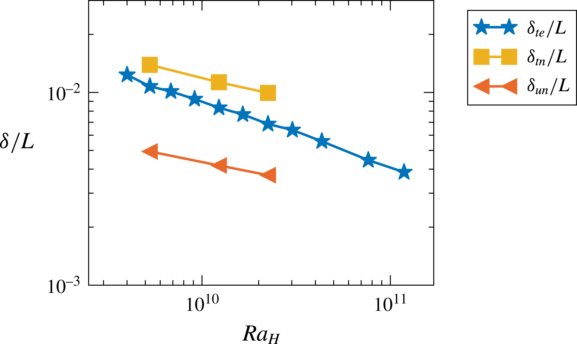
Figure 10. Normalised boundary layer thickness in the single-phase case as a function of
 $Ra_{H}$
. Here
$Ra_{H}$
. Here
 ${\unicode[STIX]{x1D6FF}_{u}}_{n}$
and
${\unicode[STIX]{x1D6FF}_{u}}_{n}$
and
 ${\unicode[STIX]{x1D6FF}_{t}}_{n}$
are numerically obtained thickness of the kinetic and thermal boundary layer, respectively. The thickness of the thermal boundary layer obtained from the experiments is given as
${\unicode[STIX]{x1D6FF}_{t}}_{n}$
are numerically obtained thickness of the kinetic and thermal boundary layer, respectively. The thickness of the thermal boundary layer obtained from the experiments is given as
 ${\unicode[STIX]{x1D6FF}_{t}}_{e}$
.
${\unicode[STIX]{x1D6FF}_{t}}_{e}$
.
As seen in figure 9(a), the mean temperature profile in the case of bubbly flow is completely different from that of single-phase flow. In the bulk, two known mixing mechanisms contribute to the distortion of the flat temperature profile that was observed in the single-phase case: (i) capture and transport by the bubble wakes (Bouche et al. Reference Bouche, Cazin, Roig and Risso2013), and (ii) dispersion by the bubble-induced turbulence, which is the dominant one as shown by Alméras et al. (Reference Alméras, Risso, Roig, Cazin, Plais and Augier2015). Near the heated and cooled walls, we visually observed the bubbles bouncing along the walls. This presumably disturbs the thermal boundary layers; however, this cannot be measured due to insufficient experimental resolution.
Figures 9(b) and 5(a,b) show that the temperature fluctuations induced by bubbles are even two orders of magnitudes higher than in the single-phase case (
 $T^{\prime }=T-\langle T\rangle$
, where
$T^{\prime }=T-\langle T\rangle$
, where
 $T^{\prime }$
is the temperature fluctuations,
$T^{\prime }$
is the temperature fluctuations,
 $T$
is the measured instantaneous temperature and
$T$
is the measured instantaneous temperature and
 $\langle T\rangle$
is the time-averaged temperature at the measurement point). The normalised standard deviations of the fluctuations in both single- and two-phase cases are higher closer to the cold and hot walls than in the centre of the set-up. This is possibly due to the temperature probe seeing more hot and cold plumes closer to the heated and cold walls, a well-known phenomenon from Rayleigh–Bénard flow (Ahlers et al.
Reference Ahlers, Grossmann and Lohse2009). Here slight asymmetry of the temperature profiles and the profiles of normalised standard deviation close to the walls must be attributed to the difference in the nature of heating and cooling of the side walls (see the asymmetry also in figure 9
a). Figure 5(a,b) also demonstrate that the time scales of fluctuations in the single- and two-phase cases are different, along with much more intense temperature fluctuations for the bubbly flow.
$\langle T\rangle$
is the time-averaged temperature at the measurement point). The normalised standard deviations of the fluctuations in both single- and two-phase cases are higher closer to the cold and hot walls than in the centre of the set-up. This is possibly due to the temperature probe seeing more hot and cold plumes closer to the heated and cold walls, a well-known phenomenon from Rayleigh–Bénard flow (Ahlers et al.
Reference Ahlers, Grossmann and Lohse2009). Here slight asymmetry of the temperature profiles and the profiles of normalised standard deviation close to the walls must be attributed to the difference in the nature of heating and cooling of the side walls (see the asymmetry also in figure 9
a). Figure 5(a,b) also demonstrate that the time scales of fluctuations in the single- and two-phase cases are different, along with much more intense temperature fluctuations for the bubbly flow.
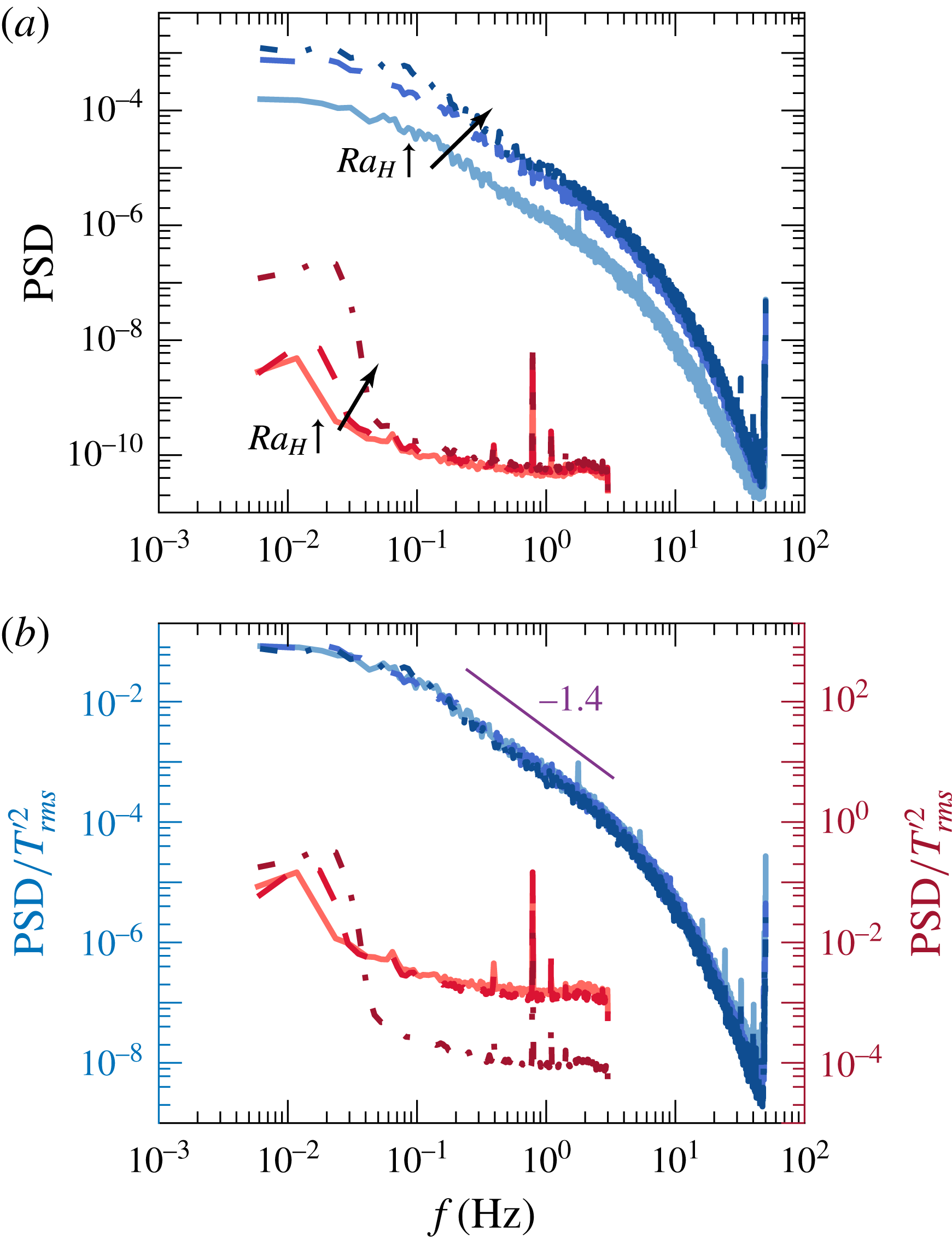
Figure 11. Raw (a) and normalised (b) power spectra of the temperature fluctuations at the centre of the set-up for single-phase (red lines) and two-phase
 $\unicode[STIX]{x1D6FC}=0.9\,\%$
(blue lines): solid line,
$\unicode[STIX]{x1D6FC}=0.9\,\%$
(blue lines): solid line,
 $Ra_{H}=5.2\times 10^{9}$
; dashed line,
$Ra_{H}=5.2\times 10^{9}$
; dashed line,
 $Ra_{H}=1.6\times 10^{10}$
; dash-dotted line,
$Ra_{H}=1.6\times 10^{10}$
; dash-dotted line,
 $Ra_{H}=2.2\times 10^{10}$
.
$Ra_{H}=2.2\times 10^{10}$
.
To explore this in better detail, we now present the power spectrum of the temperature fluctuations (‘thermal power spectrum’) for both cases. Figure 11(a) shows this power spectrum of temperature fluctuations at mid-height in the centre of the set-up for the single- and two-phase cases. In the single-phase case the measured temperature fluctuations are limited to frequencies lower than
 $10^{-1}~\text{Hz}$
. At approximately
$10^{-1}~\text{Hz}$
. At approximately
 $10^{-2}~\text{Hz}$
we observe a peak, beyond which there is a very steep decrease of the spectrum (the same frequency can be observed in figure 5
a). As is well known (Castaing et al.
Reference Castaing, Gunaratne, Heslot, Kadanoff, Libchaber, Thomae, Wu, Zaleski and Zanetti1989), this peak corresponds to the large-scale circulation frequency (
$10^{-2}~\text{Hz}$
we observe a peak, beyond which there is a very steep decrease of the spectrum (the same frequency can be observed in figure 5
a). As is well known (Castaing et al.
Reference Castaing, Gunaratne, Heslot, Kadanoff, Libchaber, Thomae, Wu, Zaleski and Zanetti1989), this peak corresponds to the large-scale circulation frequency (
 $f_{LS}\approx V_{ff}/4H$
), which can be estimated from the free fall velocity
$f_{LS}\approx V_{ff}/4H$
), which can be estimated from the free fall velocity
 $V_{ff}=\sqrt{g\unicode[STIX]{x1D6FD}\unicode[STIX]{x0394}TH}$
which is
$V_{ff}=\sqrt{g\unicode[STIX]{x1D6FD}\unicode[STIX]{x0394}TH}$
which is
 ${\sim}6~\text{cm}~\text{s}^{-1}$
for the lowest
${\sim}6~\text{cm}~\text{s}^{-1}$
for the lowest
 $Ra_{H}$
and
$Ra_{H}$
and
 ${\sim}11~\text{cm}~\text{s}^{-1}$
for the highest
${\sim}11~\text{cm}~\text{s}^{-1}$
for the highest
 $Ra_{H}$
. In both the single-phase and two-phase cases, a higher level of thermal power is seen for higher
$Ra_{H}$
. In both the single-phase and two-phase cases, a higher level of thermal power is seen for higher
 $Ra_{H}$
numbers. The same trend is seen for all the measurement positions at mid-height. If we now compare the single-phase and two-phase spectra, we can see that with the bubble injection, the thermal power of the fluctuations is increased by nearly three orders of magnitude. The bubbly flow also shows fluctuations at a range of time scales, with a gradual decay of thermal power from
$Ra_{H}$
numbers. The same trend is seen for all the measurement positions at mid-height. If we now compare the single-phase and two-phase spectra, we can see that with the bubble injection, the thermal power of the fluctuations is increased by nearly three orders of magnitude. The bubbly flow also shows fluctuations at a range of time scales, with a gradual decay of thermal power from
 $f\simeq 0.1{-}3~\text{Hz}$
. The observation that substantial power of the temperature fluctuations resides at smaller time scales, as compared to the single-phase case where the power mainly resides at the largest time scales, further confirms that the bubble-induced liquid fluctuations are the dominant contribution to the total heat transfer.
$f\simeq 0.1{-}3~\text{Hz}$
. The observation that substantial power of the temperature fluctuations resides at smaller time scales, as compared to the single-phase case where the power mainly resides at the largest time scales, further confirms that the bubble-induced liquid fluctuations are the dominant contribution to the total heat transfer.
The thermal power spectra plots in figure 11(a) show a
 $Ra_{H}$
dependence for both single- and two-phase cases. While upon normalising with the variance of temperature fluctuations
$Ra_{H}$
dependence for both single- and two-phase cases. While upon normalising with the variance of temperature fluctuations
 $T_{rms}^{\prime 2}$
in the single-phase case, we do not observe complete overlap of the spectra, possibly due to noise present at higher frequencies, in bubbly flow we observe a nearly perfect collapse of the three Rayleigh numbers (see figure 11
b). This suggests a universal behaviour for bubbly flow. Interestingly, this is similar to the velocity fluctuation spectra observed for bubbly flows (Lance & Bataille Reference Lance and Bataille1991; Riboux et al.
Reference Riboux, Risso and Legendre2010; Roghair et al.
Reference Roghair, Martinez Mercado, Van Sint Annaland, Kuipers, Sun and Lohse2011; Prakash et al.
Reference Prakash, Martínez Mercado, van Wijngaarden, Mancilla, Tagawa, Lohse and Sun2016), where a normalisation with the scale of velocity fluctuations
$T_{rms}^{\prime 2}$
in the single-phase case, we do not observe complete overlap of the spectra, possibly due to noise present at higher frequencies, in bubbly flow we observe a nearly perfect collapse of the three Rayleigh numbers (see figure 11
b). This suggests a universal behaviour for bubbly flow. Interestingly, this is similar to the velocity fluctuation spectra observed for bubbly flows (Lance & Bataille Reference Lance and Bataille1991; Riboux et al.
Reference Riboux, Risso and Legendre2010; Roghair et al.
Reference Roghair, Martinez Mercado, Van Sint Annaland, Kuipers, Sun and Lohse2011; Prakash et al.
Reference Prakash, Martínez Mercado, van Wijngaarden, Mancilla, Tagawa, Lohse and Sun2016), where a normalisation with the scale of velocity fluctuations
 $u_{rms}^{2}$
demonstrates universality. Furthermore, the same behaviour is seen at all measurement positions and all Rayleigh numbers (note that in figure 11(b), we have shown the measurements at the centre only). We also observe a clear slope of
$u_{rms}^{2}$
demonstrates universality. Furthermore, the same behaviour is seen at all measurement positions and all Rayleigh numbers (note that in figure 11(b), we have shown the measurements at the centre only). We also observe a clear slope of
 $-1.4$
at the scales
$-1.4$
at the scales
 $f\simeq 0.1{-}3~\text{Hz}$
. It remains unclear why this exact slope is present, and how it can be attributed to bubble-induced turbulence. Events occurring at shorter time scales, such as at frequencies where the
$f\simeq 0.1{-}3~\text{Hz}$
. It remains unclear why this exact slope is present, and how it can be attributed to bubble-induced turbulence. Events occurring at shorter time scales, such as at frequencies where the
 $-3$
slope is present in velocity spectra for bubble-induced turbulence, typically starting at
$-3$
slope is present in velocity spectra for bubble-induced turbulence, typically starting at
 $1/t_{pseudo}\sim 35~\text{Hz}$
(Riboux et al.
Reference Riboux, Risso and Legendre2010), would be undetectable here due to the limiting response time of the thermistor used.
$1/t_{pseudo}\sim 35~\text{Hz}$
(Riboux et al.
Reference Riboux, Risso and Legendre2010), would be undetectable here due to the limiting response time of the thermistor used.
5 Summary of main results and discussion
An experimental study on heat transport in homogeneous bubbly flow has been conducted. The experiments are performed in a rectangular bubble column heated from one side and cooled from the other (see figure 1). Two parameters are varied: the gas volume fraction and the Rayleigh number. The gas volume fraction ranges from
 $0\,\%$
to
$0\,\%$
to
 $5\,\%$
, and the bubble diameters are approximately
$5\,\%$
, and the bubble diameters are approximately
 $2.5~\text{mm}$
. The Rayleigh number is in the range
$2.5~\text{mm}$
. The Rayleigh number is in the range
 $4.0\times 10^{9}{-}1.2\times 10^{11}$
.
$4.0\times 10^{9}{-}1.2\times 10^{11}$
.
First, we focus on characterisation of the global heat transfer for single-phase and two-phase cases. We find that two completely different mechanisms govern the heat transport in these two cases. In the single-phase case, the vertical natural convection is driven solely by the imposed difference between the mean wall temperatures. In this configuration the temperature acts as an active scalar driving the flow. The Nusselt number increases with increasing Rayleigh number, and as expected effectively scales as
 $\overline{Nu}\sim Ra_{H}^{0.33}$
(see figure 6
a). However, in the case of homogeneous bubbly flow the heat transfer comes from two different contributions: natural convection driven by the horizontal temperature gradient and the bubble-induced diffusion, where the latter dominates. This is substantiated by our observations that the Nusselt number in bubbly flow is nearly independent of the Rayleigh number and depends solely on the gas volume fraction, evolving as
$\overline{Nu}\sim Ra_{H}^{0.33}$
(see figure 6
a). However, in the case of homogeneous bubbly flow the heat transfer comes from two different contributions: natural convection driven by the horizontal temperature gradient and the bubble-induced diffusion, where the latter dominates. This is substantiated by our observations that the Nusselt number in bubbly flow is nearly independent of the Rayleigh number and depends solely on the gas volume fraction, evolving as
 $\overline{Nu}\propto \unicode[STIX]{x1D6FC}^{0.45}$
(see figure 8). We thus find nearly the same scaling as in the case of the mixing of a passive tracer in a homogeneous bubbly flow for a low gas volume fraction (Alméras et al.
Reference Alméras, Risso, Roig, Cazin, Plais and Augier2015), which implies that the bubble-induced mixing is indeed limiting the efficiency of the heat transfer.
$\overline{Nu}\propto \unicode[STIX]{x1D6FC}^{0.45}$
(see figure 8). We thus find nearly the same scaling as in the case of the mixing of a passive tracer in a homogeneous bubbly flow for a low gas volume fraction (Alméras et al.
Reference Alméras, Risso, Roig, Cazin, Plais and Augier2015), which implies that the bubble-induced mixing is indeed limiting the efficiency of the heat transfer.
We further performed local temperature measurements at the mid-height of the set-up for gas volume fractions of
 $\unicode[STIX]{x1D6FC}=0\,\%$
and
$\unicode[STIX]{x1D6FC}=0\,\%$
and
 $\unicode[STIX]{x1D6FC}=0.9\,\%$
, and for Rayleigh numbers
$\unicode[STIX]{x1D6FC}=0.9\,\%$
, and for Rayleigh numbers
 $5.2\times 10^{9}$
,
$5.2\times 10^{9}$
,
 $1.6\times 10^{10}$
and
$1.6\times 10^{10}$
and
 $2.2\times 10^{10}$
. For single-phase flow, we observe that the mean temperature remains constant in the bulk at mid-height. However, in the two-phase flow case, this is completely obstructed by the mixing induced by the bubbles. Injection of bubbles induces up to 200 times stronger temperature fluctuations (see figure 9
b). These fluctuations over a wide spectrum of frequencies (see figure 11) are thus the signature of the heat transport enhancement due to bubble injection. A clear slope of
$2.2\times 10^{10}$
. For single-phase flow, we observe that the mean temperature remains constant in the bulk at mid-height. However, in the two-phase flow case, this is completely obstructed by the mixing induced by the bubbles. Injection of bubbles induces up to 200 times stronger temperature fluctuations (see figure 9
b). These fluctuations over a wide spectrum of frequencies (see figure 11) are thus the signature of the heat transport enhancement due to bubble injection. A clear slope of
 $-1.4$
at the scales
$-1.4$
at the scales
 $f\simeq 0.1{-}3~\text{Hz}$
was also observed. In order to understand why this slope is present in that range it would be beneficial to perform local velocity measurements in the flow with heating, which is an objective of our future studies. Further examination with fully resolved numerical simulations will also help us understand the effect of bubbles. These simulations are planned for future work, as well.
$f\simeq 0.1{-}3~\text{Hz}$
was also observed. In order to understand why this slope is present in that range it would be beneficial to perform local velocity measurements in the flow with heating, which is an objective of our future studies. Further examination with fully resolved numerical simulations will also help us understand the effect of bubbles. These simulations are planned for future work, as well.
Figure 12. Extrapolation of the Nusselt number to high Rayleigh numbers for the two-phase case (dashed lines, lowest and highest studied
 $\unicode[STIX]{x1D6FC}$
), and the single-phase case (dotted line). A cross-over between the extrapolated single- and two-phase cases occurs at
$\unicode[STIX]{x1D6FC}$
), and the single-phase case (dotted line). A cross-over between the extrapolated single- and two-phase cases occurs at
 $Ra_{H}\approx 1.2\times 10^{12}$
for
$Ra_{H}\approx 1.2\times 10^{12}$
for
 $\unicode[STIX]{x1D6FC}=0.5\,\%$
, and at
$\unicode[STIX]{x1D6FC}=0.5\,\%$
, and at
 $Ra_{H}\approx 4\times 10^{13}$
for
$Ra_{H}\approx 4\times 10^{13}$
for
 $\unicode[STIX]{x1D6FC}=5\,\%$
. However, as we approach these
$\unicode[STIX]{x1D6FC}=5\,\%$
. However, as we approach these
 $Ra_{H}$
, we expect the Rayleigh-independent trends of Nusselt number to change, namely to increase with increasing
$Ra_{H}$
, we expect the Rayleigh-independent trends of Nusselt number to change, namely to increase with increasing
 $Ra_{H}$
.
$Ra_{H}$
.
To conclude, we observe up to 20 times heat transfer enhancement due to bubble injection (see figure 6
b). This demonstrates that the diffusion induced by bubbles is a highly effective mechanism for heat transfer enhancement. Nevertheless, several questions remain unanswered. One question of great practical importance is: At what Rayleigh number will the contribution of natural convection to the total heat transfer become comparable or even greater than the contribution of bubble-induced turbulence? If we extrapolate the data to higher Rayleigh numbers, we can obtain the maximum expected value of
 $Ra_{H}$
at which the two contributions are comparable (see dashed lines in figure 12). This occurs at
$Ra_{H}$
at which the two contributions are comparable (see dashed lines in figure 12). This occurs at
 $Ra_{H}\approx 1.2\times 10^{12}$
for
$Ra_{H}\approx 1.2\times 10^{12}$
for
 $\unicode[STIX]{x1D6FC}=0.5\,\%$
and at
$\unicode[STIX]{x1D6FC}=0.5\,\%$
and at
 $Ra_{H}\approx 4\times 10^{13}$
for
$Ra_{H}\approx 4\times 10^{13}$
for
 $\unicode[STIX]{x1D6FC}=5\,\%$
. As we approach these
$\unicode[STIX]{x1D6FC}=5\,\%$
. As we approach these
 $Ra_{H}$
, we expect the Rayleigh-independent behaviour of Nusselt number to change. Presumably, when
$Ra_{H}$
, we expect the Rayleigh-independent behaviour of Nusselt number to change. Presumably, when
 $Ra_{H}$
is sufficiently large, the Nusselt number will increase with
$Ra_{H}$
is sufficiently large, the Nusselt number will increase with
 $Ra_{H}$
even for the two-phase cases. Based on our current knowledge, it is difficult to predict at what
$Ra_{H}$
even for the two-phase cases. Based on our current knowledge, it is difficult to predict at what
 $Ra_{H}$
this trend will change. This calls for future investigations spanning a wider range of control parameters.
$Ra_{H}$
this trend will change. This calls for future investigations spanning a wider range of control parameters.
Acknowledgements
We thank G.-W. Bruggert, M. Bos and B. Benschop for technical support and Y.-C. Xie for the help with the experimental technique. This work is part of the Industrial Partnership Programme i36 Dense Bubbly Flows that is carried out under an agreement between Akzo Nobel Chemicals International B.V., DSM Innovation Center B.V., SABIC Global Technologies B.V., Shell Global Solutions B.V., Tata Steel Nederland Technology B.V. and the Netherlands Organisation for Scientific Research (NWO). We also thank STW foundation of the Netherlands, European High-Performance Infrastructures in Turbulence (EuHIT), and COST Action MP1305 for support. This work was also supported by The Netherlands Center for Multiscale Catalytic Energy Conversion (MCEC), an NWO Gravitation Programme funded by the Ministry of Education, Culture and Science of the government of The Netherlands. Part of the simulations were carried out on the Dutch national e-infrastructure with the support of SURF Cooperative. We also acknowledge PRACE for awarding us access to Marconi at CINECA, Italy under PRACE project number 2016143351, and DECI resource ARCHER UK National Supercomputing Service with the support from PRACE under project 13DECI0246. C.S. acknowledges the financial support from Natural Science Foundation of China under Grant no. 11672156.


 Open access