


1. Introduction
Several decades of internal wave field observations have exposed the apparent existence of a universal internal wave continuum, the Garrett–Munk (GM) spectrum (Garrett & Munk Reference Garrett and Munk1975). The GM spectrum is conventionally thought of as the manifestation of the internal wave energy cascade from the large-scale input (Garrett & Kunze Reference Garrett and Kunze2007) to much smaller spatio-temporal scales where internal waves mix the ocean (Wunsch & Ferrari Reference Wunsch and Ferrari2004). Understanding the physical processes involved in the internal wave energy cascade – sometimes referred to as internal wave turbulence (Zakharov, Lvov & Falkovich Reference Zakharov, Lvov and Falkovich1992) – remains a challenge (Lvov, Polzin & Tabak Reference Lvov, Polzin and Tabak2004; MacKinnon et al. Reference MacKinnon2017; Dauxois et al. Reference Dauxois, Joubaud, Odier and Venaille2018). This study investigates the contribution of wave attractors to the energy cascade.
A basic property of linear internal waves in a stratified fluid with a linear density profile is the conservation of the propagation angle, even when reflecting from boundaries (e.g. Sutherland Reference Sutherland2010). As a consequence, reflections at inclined boundaries lead to focusing or defocusing, corresponding to a shift of spectral energy density towards smaller or larger spatial scales, respectively. Notably, focusing typically dominates over defocusing for reflections from both subcritical bottom topography (Bühler & Holmes-Cerfon Reference Bühler and Holmes-Cerfon2011) and supercritical topographies (Mathur, Carter & Peacock Reference Mathur, Carter and Peacock2014) as well as in fully confined basins having non-trivial shape (Maas & Lam Reference Maas and Lam1995). The domination of focusing occurs because the former lead to amplification, the latter to a reduction of wave amplitude. In a confined basin, waves can defocus upon subsequent reflections from the boundary until reaching the basin scale. From that moment on, these waves start to focus again. They add to waves that were already focusing from the beginning. Focusing thus determines the ultimate fate of enclosed waves in an ideal fluid setting. Hence, repeated reflections of internal waves at topography can cascade energy to smaller, dissipative spatial scales. This process is especially interesting if the trajectory of the internal waves converges to a closed loop, such that the energy accumulates along so-called wave attractors (Maas & Lam Reference Maas and Lam1995; Maas et al. Reference Maas, Benielli, Sommeria and Lam1997). The linear dynamics of wave attractors in two-dimensional trapezoidal domains has been studied thoroughly for inviscid (Maas Reference Maas2005) and viscous flows (Hazewinkel et al. Reference Hazewinkel, van Breevoort, Dalziel and Maas2008, Reference Hazewinkel, Tsimitri, Maas and Dalziel2010). More realistic open-ocean topographies admitting wave attractors are investigated by Tang & Peacock (Reference Tang and Peacock2010), Echeverri et al. (Reference Echeverri, Yokossi, Balmforth and Peacock2011) and Guo & Holmes-Cerfon (Reference Guo and Holmes-Cerfon2016) using quasi two-dimensional settings. While it remains challenging to understand wave attractors in truly three-dimensional domains (Drijfhout & Maas Reference Drijfhout and Maas2007; Pillet et al. Reference Pillet, Ermanyuk, Maas, Sibgatullin and Dauxois2018), it has become evident that complicated ocean topographies do not preclude the existence of wave attractors (Sibgatullin & Ermanyuk Reference Sibgatullin and Ermanyuk2019).
It is well established that, for large-scale monochromatic energy input, the attractor's energy cascade can terminate with viscous dissipation (Ogilvie Reference Ogilvie2005; Hazewinkel et al. Reference Hazewinkel, van Breevoort, Dalziel and Maas2008; Beckebanze et al. Reference Beckebanze, Brouzet, Sibgatullin and Maas2018) and/or result in triadic resonant instability (TRI) if the energy input is sufficiently large (Scolan, Ermanyuk & Dauxois Reference Scolan, Ermanyuk and Dauxois2013; Brouzet et al. Reference Brouzet, Ermanyuk, Joubaud, Pillet and Dauxois2017). Brouzet et al. (Reference Brouzet, Ermanyuk, Joubaud, Sibgatullin and Dauxois2016, Reference Brouzet, Ermanyuk, Joubaud, Pillet and Dauxois2017) and Brunet, Dauxois & Cortet (Reference Brunet, Dauxois and Cortet2019) show experimentally that, in the large-amplitude regime, a wave attractor can lead to an energy cascade where repeated geometric focusing amplifies the wave field locally near the wave attractor until a threshold is passed, after which TRI sets in. (The presence of a threshold relates to the finite width of the wave beam Bourget et al. (Reference Bourget, Scolan, Dauxois, Le Bars, Odier and Joubaud2014) due to its geometric focusing.) TRI projects energy from the monochromatic input frequency  $\omega _1$ to the new frequencies (
 $\omega _+,\omega _-$) such that
  $\omega _1 = \omega _+ + \omega _-$. (Historically, the case
 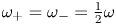 $\omega _+=\omega _-=\frac {1}{2} \omega$, known as parametric subharmonic instability (Dauxois et al. Reference Dauxois, Joubaud, Odier and Venaille2018) was studied.) However, the interaction may also be reversed. Two input waves of the same or different frequency may – without any threshold – interact and lead to a new output frequency, satisfying the more general relationship
  $\pm \omega _1 \mp \omega _\pm = \pm \omega _{-}$, a process referred to as two wave interactions (TWIs) (Davis et al. Reference Davis, Jamin, Deleuze, Joubaud and Dauxois2020). Note that, here, both
  $\pm \omega _1$ and
  $\mp \omega _+$ are now the input frequencies. The notation of
  $\omega _\pm$ has been chosen to avoid confusion with
  $\omega _k$ defined in table 1. For clarity, both TRI and TWI are predicated on triadic resonances. For TRI, some of the energy supplied through one input wave is emitted through two daughter waves. For TWI, some of the energy supplied through two input waves is transferred to a single daughter wave. (There may also be some transfer of energy from the higher frequency input wave to the lower frequency one as a result of the TWI.)
Table 1. Parameter values of the laboratory experiments. The  $K$ individual waves in the most energetic experiments for the multi-frequency wave field are forced with amplitude
  $A/\sqrt {K} = 11.5/4=2.87\ \textrm {mm}$ to prevent the maximum amplitude, due to the summation of 16 waves, exceeding 17 mm – the threshold for ASWaM.

For two reasons, geometric focusing projects only a small fraction of the oceanic internal wave continuum onto simple wave attractors. These simple attractors are characterized by a periodic orbit with a small number of surface and supercritical bottom reflections and by a short perimeter. Firstly, the spectral widths of the frequency bands that allow these simple (‘short’ path-length) wave attractors are narrow and sparsely distributed within the internal wave continuum, corresponding to complicated, ‘long’ path-length wave attractors that are prone to viscous degradation. This is due to the ocean's small aspect ratio. Secondly, oceanic internal wave forcing is particularly strong at a discrete set of tidal frequencies (as opposed to being part of a broad-band continuum). These tidal frequencies would need to fall into one of these narrow bands in order to excite a simple attractor directly (Echeverri et al. Reference Echeverri, Yokossi, Balmforth and Peacock2011; Guo & Holmes-Cerfon Reference Guo and Holmes-Cerfon2016). These considerations illustrate that it is unlikely that the internal wave energy cascade proposed by Brouzet et al. (Reference Brouzet, Ermanyuk, Joubaud, Sibgatullin and Dauxois2016) applies to the ocean. It seems more realistic that frequency bands corresponding to simple wave attractors are at best reached by a sequence of TWIs.
In a series of laboratory experiments we study both single- and multi-frequency forcings that correspond to attractors over a range of amplitudes in a trapezoidal domain. We first consider the simple case of weak (linear) monochromatic forcing, where attractors are easily identified using classical methods. We then increase the forcing amplitude and examine weakly nonlinear monochromatic forcing, where we find that the attractor beam becomes unstable to TRI. Nevertheless, we can show that geometric focusing onto wave attractors persists in this regime, even though the attractors are not directly visible. We then consider low-amplitude multi-frequency forcing. Again, despite patterns of wave attractors not being immediately visible, by examining the energy spectra at dissipative length scales we can see that geometric focusing has occurred at frequencies that correspond to attractors. Finally, we examine larger-amplitude forcing in the multi-frequency domain. In contrast to the TRI mechanism based on single-frequency forcing, in this regime we observe that multi-frequency forcing leads to linear geometric focusing, mixing and to TWIs. The waves triadically generated by TWI may themselves fall into frequency bands corresponding to simple attractors which may lead to their subsequent amplification. However, as the forcing amplitude was not high enough to generate TRI in this regime, dissipation prevails because TWI and geometric focusing are simultaneously present. Since geometric focusing is a linear process, it takes precedence over nonlinear processes involved in TRI which requires a further boost in the amplitude of the internal wave field.
The structure of this paper is as follows. In § 2 we report the laboratory set-up, including a detailed description of the multi-frequency, large-scale forcing by a newly developed wavemaker. The experimental results along with discussion are presented in § 3 broken down by either monochromatic (§ 3.1) or multi-frequency (§ 3.2) forcing and by amplitude. Finally, conclusions are drawn in § 4.
2. Experimental set-up
We employ the Long Flow Tank (11.4 m long,  $W=25.5$ cm wide) in the G. K. Batchelor Laboratory, DAMTP, University of Cambridge. A salt stratification with linear density profile giving a constant buoyancy frequency
  $N = 1.695 \pm 0.08\ \textrm {rad}\ \textrm {s}^{-1}$ is created over 8 h by two computer-controlled gear pumps to a depth of approximately 43 cm. Using gear pumps proves to be more convenient than the traditional double-bucket method as it avoids the need for large reservoirs of fresh and salt water, and allows the specification of the water depth and buoyancy frequency to be made more accurately before commencing filling. The stratification is described by the buoyancy frequency defined by
 \begin{equation} N^2 ={-} \frac{g}{\rho_0}\frac{\textrm{d}\bar{\rho}}{\textrm{d}z} \end{equation}
for a fluid in which the density  $\rho$ is given as the sum of a background density
  $\rho _0 + \bar {\rho }(z)$ (varying linearly with depth) and a spatio-temporal perturbation
  $\rho '(x,z,t)$ representing the internal waves, where (x, z) is the Cartesian coordinate system: x points along the length of the wavemaker and
  $z$ points upwards, opposing gravity. Here,
  $g = 9.81\ \textrm {m}\ \textrm {s}^{-2}$ is the gravitational acceleration and
  $\rho _0 = 10^3\ \textrm {kg}\ \textrm {m}^{-3}$ is the reference density. The stratification is measured using an aspirating conductivity probe traversed through the depth (the tip of this probe can be seen in figure 1). After filling, two barriers are lowered along pre-installed tracks. One barrier is vertical, the second sloping at angle
  $\alpha =45^{\circ }\pm 0.1^{\circ }$ with respect to the horizontal, forming a trapezoidal domain with water depth
  $H = 42.7\pm 0.3\ \textrm {cm}$, bottom length
  $L_b=103\pm 0.1\ \textrm {cm}$ and surface length
  $L_s=L_b + H \cot \alpha = 145.7\pm 0.3\ \textrm {cm}$. A slope of
  $45^{\circ }$ was chosen as steeper angles would have reduced the frequency range capable of forming an attractor, while shallower slopes would have resulted in more of the experiment being outside the field of view of the camera. The 1 m long Arbitrary Spectrum Wave Maker (ASWaM) (Dobra, Lawrie & Dalziel Reference Dobra, Lawrie and Dalziel2019) is located at the bottom of the trapezoidal domain. The ASWaM generates fluid perturbations by pushing the elastic bottom (nylon-faced neoprene foam) from below with 96 rods (each 4 mm in diameter) that are connected to linear actuators (see figure 1). All actuators are individually computer controlled, allowing generation of a wide range of spatio-temporal inputs, although for the purposes of this paper we only force at one particular wavelength. The maximum half peak-to-peak amplitude is 17 mm. The length of ASWaM was used to force one wavelength, setting the wavelength,
  $L_0 = 96\ \textrm {cm}$. Glycerol – being denser than salt water – sits below the neoprene foam to prevent salt water ingress around the seals of the vertical rods connecting the actuators. For large-amplitude forcing, contamination by glycerol of the fluid column above the neoprene unfortunately did occur along with a mixed boundary layer, further discussed in § 3.2. Other wavemaker configurations could partly mitigate this by having a surface-mounted wavemaker (Bourget et al. Reference Bourget, Scolan, Dauxois, Le Bars, Odier and Joubaud2014; Supekar & Peacock Reference Supekar and Peacock2019; Boury, Odier & Peacock Reference Boury, Odier and Peacock2020) that would not require the addition of a glycerol layer.

Figure 1. Photograph of the trapezoidal section of the uniformly stratified tank enclosed by vertical and sloping barriers. Along the bottom boundary lies the Arbitrary Spectrum Wavemaker (ASWaM), comprised of 96 horizontal rods, covered in neoprene, whose vertical displacement can be individually controlled.
The internal wave motion is captured at  $4$ frames per second using synthetic schlieren (Sutherland et al. Reference Sutherland, Dalziel, Hughes and Linden1999; Dalziel, Hughes & Sutherland Reference Dalziel, Hughes and Sutherland2000) with a 12 Mega-pixel monochrome camera, positioned
  $379.3 \pm 0.5\ \textrm {cm}$ from the tank. This technique utilizes the fact that for salt water there is an approximately linear relationship between density and refractive index and so propagating internal waves distort the image observed by the camera through the tank, making the dot pattern appear to move. The camera then records this apparent displacement of the random dot pattern, which is positioned
  $15 \pm 0.5\ \textrm {cm}$ behind the tank and illuminated by a white LED panel to create a sharp pattern contrast. DigiFlow (Dalziel Reference Dalziel2006) is used to calculate the cross-tank mean of the gradient
  $\boldsymbol {\nabla } \rho ' = [\partial _x, \partial _z] \rho '$ of the density perturbation
  $\rho '$ by matching the apparently displaced pattern to the quiescent undisturbed pattern. In this paper, we express density perturbations in terms of the buoyancy
  $b =- g \rho '/\rho _0$. The limiting factor for the spatial resolution was controlled by the dot spacing used for pattern matching (Dalziel et al. Reference Dalziel, Hughes and Sutherland2000). Here, the smallest length scale resolvable was therefore approximately 2 mm for quasi-linear internal waves. We note that this measurement technique cannot resolve three-dimensional structure due to localized wave breaking.
An attractor with  $m$ surface reflections and
  $n$ sidewall reflections is referred to as an (
 $m,n$)-attractor (Maas & Lam Reference Maas and Lam1995). Hence, the simplest, diamond-shaped wave attractor (see figure 2a) with one reflection from each of the four planar boundaries is the (1,1)-attractor. For the multiple-frequency forcing experiments, the frequency range is chosen to be slightly wider than the (1,1)-attractor band.

Figure 2. (a) Sketch of the trapezoidal fluid domain with diamond-shaped (1,1)-attractor (orange) and the two degenerate (1,1)-attractors (dashed and dotted lines) at the edges of the attractor frequency range  $I_{(1,1)}$ defined by (2.2). The wavemaker is indicated by the sinusoidal bottom perturbation. (b) Conceptual illustration of the wave attractor energy cascade in wave frequency (
 $\omega$) – wavenumber (
 $k$) space. Geometric focusing of large-scale energy input within a
  $(m,n)$-attractor frequency band
  $I_{(m,n)}$ pumps up the energy density at smaller scales until reaching the dissipative range. The initial increase in energy density permits weakly nonlinear TRI and TWI to redistribute wave energy to different frequencies, including those outside the
  $I_{(m,n)}$-band.
Throughout this paper, we express the internal wave dispersion relation as  $\omega = N \sin \theta$, where
  $\omega$ is the wave frequency and
  $\theta$ is the angle that the lines of constant phase make with the horizontal. The smallest possible angle for a (1,1)-attractor is
  $\theta _{min} = \sin ^{-1}( H/\sqrt {H^2+L_s^2} ) = 16.3^{\circ }$, and largest possible angle is
  $\theta _{max} = \sin ^{-1} (H/\sqrt {H^2+L_b^2}) = 22.5^{\circ }$. The corresponding degenerate attractors are shown by the red dotted and blue dashed lines in figure 2(a), respectively. The thick orange diamond in figure 2(a) shows an intermediate (1,1)-wave attractor with angle
  $\theta = \sin ^{-1} (H/\sqrt {H^2+((L_b+L_s)/2)^2}) = 19.0^{\circ }$.
For a trapezoidal fluid domain, the theoretical frequency band for (1,1)-wave attractors is
 \begin{equation} I_{(1,1)} = N[ \sin(\theta_{min}), \sin(\theta_{max})] = N \left[\frac{H}{\sqrt{H^2+L_s^2}}, \frac{H}{\sqrt{H^2+L_b^2}}\right].\end{equation}
For our laboratory set-up we get the frequency band  $I_{(1,1)}=[0.471, 0.640]\ \textrm {rad}\ \textrm {s}^{-1}$, with an uncertainty for the lower and upper bound of approximately 5 % due to uncertainties in the buoyancy frequency
  $N = 1.695 \pm 0.08\ \textrm {rad}\ \textrm {s}^{-1}$. The degenerate wave attractors corresponding to the edges of the frequency band are special in the sense that its two remaining branches overlap, i.e. on either side energy propagates in opposite directions. This will also be the case for the associated oscillatory currents, leading to shear instabilities. For this reason, we expect wave attractors to appear only for wave frequencies that fall well within the theoretical frequency band. We present here two series of six laboratory experiments, listed in table 1.
For both the single- and multi-frequency forcing experiments, the neoprene foam at  $z=-H + h(x,t)$ (see sketch figure 2a) is displaced by imposing
 \begin{gather} h(x,t) = \begin{cases} A g(x) f(t), & L_b-L_0< x < L_b \\ 0 , & 0 < x < L_b-L_0 \end{cases}\\ \mbox{for} \ g(x) =\sin\left(k_0 (x-L_b+L_0) \right) \left( 1 - \exp({-c (x-L_b+L_0)}) - \exp({-c(L_b-x)}) \right). \nonumber \end{gather}
Here,  $t$ is time,
  $k_0 = 2{\rm \pi} /L_0$ is the imposed horizontal wavenumber such that the wavelength is equal to the length
  $L_0 = 96\ \textrm {cm}$ of the ASWaM, and
  $c=10\ \textrm {m}^{-1}$ is an edge-smoothing parameter. The small region,
  $L_b - L_0 = 7\ \textrm {cm}$, defines the horizontal, solid boundary bottom section to the left of ASWaM in figure 2. The relative amount of energy input at wavelengths smaller than
  $L_0$, was considered negligible due to smoothing. This was most difficult to achieve at the connection point between the sloping barrier and the base of the tank. A smooth rubber foot was placed at the bottom of the metal tracks while a piece of acetate was attached to the barrier to ensure a smooth transition at this corner. A small amount of internal wave generation still occurred at the edge regions, however, they were quickly damped by viscosity due to their high wavenumbers.
We vary the amplitude  $A$ among experiments (see table 1) to experimentally investigate the transition from small-amplitude to large-amplitude regimes.
For  $K \ge 1$ distinct input frequencies (
 $\omega _k, k=1,\ldots ,K$) we use the time dependence given by
 \begin{equation} f(t) = \begin{cases} 0 & \mbox{for} \ t < 0\ \mbox{s} \ \mbox{and} \ t \geq 960\ \mbox{s},\\ \dfrac{t}{30 \sqrt{K}} \,\sum\limits_{k=1}^{K} \sin[\omega_k t + \phi_k)] & \mbox{for} \ 0 \leq t < 30\ \mbox{s}, \\ \dfrac{1}{\sqrt{K}} \, \sum\limits_{k=1}^{K} \sin[\omega_k t + \phi_k)] & \mbox{for} \ 30 \leq t < 930\ \mbox{s}, \\ \dfrac{(960-t)}{ 30\sqrt{K}} \,\sum\limits_{k=1}^{K} \sin[\omega_k t + \phi_k)] & \mbox{for} \ 930 \leq t < 960\ \mbox{s} . \end{cases} \end{equation}
The random phase shifts  $\phi _k$ with uniform distribution in
  $[0, 2{\rm \pi} ]$ (but kept constant for all runs), ensure that the generated wave field is not synchronous. For monochromatic forcing (
 $K=1$), the phase shift is
  $\phi _1=0$. It is found that for the experiments presented here, a steady state is reached within approximately 5 min, i.e. within 1/3 of the 16 minute duration of the experiments. Note that the energy input per frequency
  $\omega _k$ is proportional to
  $\omega _k^2 A^2/K$, therefore the higher the frequency, the higher the energy input is at that particular frequency. This kinetic energy input of the wavemaker partitions in leftward and rightward propagating wave beams (each propagating half of the energy imparted), and is converted into potential energy and back into kinetic energy within the wave beams. The total characteristic amplitude
  $A$ therefore quantifies the total energy input (
 $\propto A^2$) by ASWaM, independent of the number of frequencies
  $K$ that are used (provided the mean frequency
  $\sqrt { \sum \omega _k^2/K }$ is independent of
  $K$). The amplitude per frequency
  $\omega _k$ is therefore given by
  $A/\sqrt {K}$. We note that the internal wave generation need not be 100 % efficient (Mercier et al. Reference Mercier, Martinand, Mathur, Gastiauw, Peacock and Dauxois2010). Dobra (Reference Dobra2018) found the efficiency for ASWAM to range from 0.1 to 0.9, depending on the propagation angle
  $\theta$. One could extend the theoretical analysis by replacing
  $A/\sqrt {K}$ by
  $q_k A/\sqrt {K}$ where
  $q_k<1$ are empirical factors quantifying the wave generation efficiency per wave frequency
  $\omega _k$. We kept the analysis simple by assuming
  $q_k=1$.
3. Experimental results
3.1. Single-frequency forcing
We excite monochromatic (1,1)-attractors with single frequency  $\omega _1 = 0.55\ \textrm {rad}\ \textrm {s}^{-1}$ (
 $\theta =19.3^{\circ }$) for six different forcing amplitudes ranging from 0.5 mm to 16 mm, shown in table 1. Snapshots of the experimentally observed horizontal buoyancy gradient
  $\partial _x b$ for a weak-amplitude experiment (
 $A = 0.5\ \textrm {mm}$) and a large-amplitude experiment (
 $A=8\ \textrm {mm}$) are shown in figures 3(a,c,e,g) and 3(b,d,f,h), respectively. The time step between these panels corresponds to approximately 1.5 min. The time averages of the magnitude of the buoyancy gradient,
  $|\boldsymbol {\nabla } b | = \sqrt {|\partial _x b|^2+|\partial _z b|^2}$, for these snapshots are given in figure 3(i,j). The corresponding time series along a vertical transect at
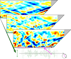
  $x_0 = 50$ cm are shown in figure 3(k) for the small amplitude and in figure 3(l) for the large amplitude. The last row of panels (figure 3m,n) depicts the non-dimensionalized prescribed forcing from ASWaM. For the small-amplitude forcing, every time snapshot shows energy localization along a diamond-shaped (1,1) wave attractor. This is again clear in the time average of these plots (figure 3i) along with the corresponding time series (figure 3k). For the larger-amplitude experiment, the time average (figure 3j) also vaguely shows energy localization along the same attractor shape. However, it is much harder to identify the presence of a wave attractor from the snapshots in figure 3(b,d,f,h) for the large-amplitude forcing, or from the corresponding time series, figure 3(l).

Figure 3. Snapshots of experimentally observed horizontal buoyancy gradient  $\partial _x b$, at times
  $t=479 + 16n{\rm \pi} /0.55$ s, where
  $n=1,\ldots ,4$, (9.50 to 14.07 min) for single-frequency forcing. (a,c,e,g) correspond to small-amplitude (
 $A=0.5$ mm) forcing, (b,d,f,h) to large-amplitude, (
 $A=8$ mm) forcing. See table 1 for experimental parameters. (i,j) Time-averaged magnitude
  $\sqrt {|\partial _x b|^2+|\partial _z b|^2}$ of the four plots above. (k,l) Time series along the vertical transect at
  $x_0=50$ cm, in (a–h) indicated by dashed lines. In (k,l), times of snapshots (a–h) are indicated by dashed vertical lines. (m,n) Time series of the non-dimensionalized bottom disturbance by ASWaM,
  $f(t)$, given by (2.4), which is regular for this single-frequency forcing.
The classical methodology of identifying attractors by local energy intensification apparently fails in the large-amplitude regime, especially when observing along a single vertical transect only. Yet, as we will see in figure 4, we can identify the wave attractors in the spatio-temporal spectra of the magnitude of the buoyancy gradient taken from the vertical transect time series at  $x_0 = 50$ cm. We verified that the spectral decompositions in figure 4 are only weakly dependent on the horizontal location of the vertical transect (not shown). Here we also present the spatio-temporal plot for the largest forcing amplitude at
  $A = 16\ \textrm {mm}$ (figure 4c). Increased energy levels at dissipative length scales corresponding to the forcing frequency of the attractor indicates a focusing reflection mechanism that contributes to the energy cascade. The smallest and most energetic wavelength of a linear attractor attainable before viscous damping begins to dominate over the focusing, denoted
  $\lambda _{min}$, is given by
  $\lambda _{min} = 2{\rm \pi} ( {\nu L_a \tan \theta }/({2 \omega (\gamma ^3-1))})^{{1}/{3}}$ with
  $\gamma = \sin (\alpha +\theta ) / \sin (\alpha -\theta ) \approx 2.08$,
  $\theta$ = 19.3
 $^{\circ }$,
  $\nu =$ 1 mm/s and
  $L_a$ the perimeter length along the attractor (Hazewinkel et al. Reference Hazewinkel, van Breevoort, Dalziel and Maas2008; Beckebanze et al. Reference Beckebanze, Brouzet, Sibgatullin and Maas2018). For our laboratory setting with
  $L_a \approx 2.5\ \textrm {m}$, this length scale is approximately 2.9 cm. Scales smaller than this are thus strongly damped due to viscous dissipation. Beckebanze et al. (Reference Beckebanze, Brouzet, Sibgatullin and Maas2018) show that for certain geometries, dissipation from friction at lateral walls can be significant. We note that for the experimental set-up presented here, the thickness of the boundary layer, which is given as
  $d_0 = \mu ^{-1}({\nu }/{\omega })^{{1}/{2}}$, where
  $\mu = \sqrt {(|{\sin ^2 \alpha }/{\sin ^2 \theta } -1|)}$, is approximately 0.7 mm. This leads to a moderate enhancement of dissipation and small increase in the minimum size (wave length) of the attractor. To be on the safe side, we have chosen dissipation to be characterized by scales between
  $1$ and 2 cm, the former limit being closer to the resolution of synthetic schlieren.

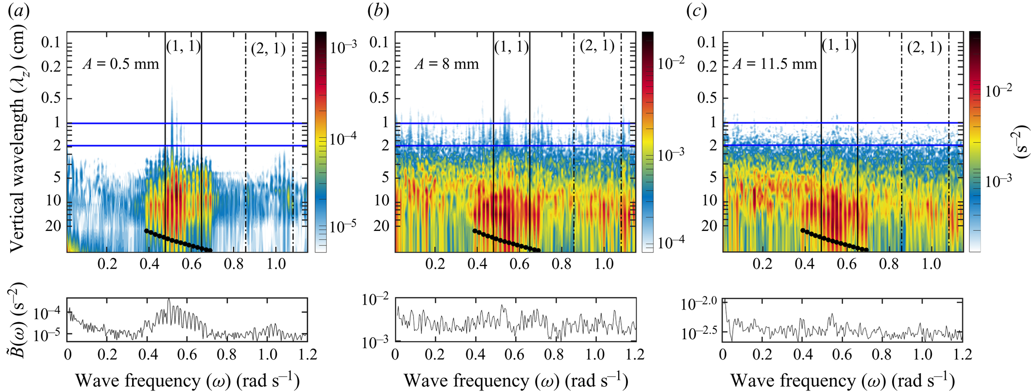
Figure 4. Spectral decompositions of the magnitude of the buoyancy gradient  $|\boldsymbol {\nabla } b(x_0,z,t)|= \sqrt {|\partial _x b|^2 +|\partial _z b|^2}$ along the vertical transect at
  $x_0=50$ cm for single-frequency forcing amplitudes
  $A = 0.5$, 8, 16 mm (a–c). The contour plots show the spatio-temporal spectra
  $\hat {B}(\omega ,\lambda _z) =({1}/{\Delta T})({1}/{H})\int _{-H}^0 \int _{T_0}^{T_1} |\boldsymbol {\nabla } b| \exp ({\textrm {i} \omega t + \textrm {i} 2{\rm \pi} /\lambda _z z})\,\textrm {d}t\,\textrm {d}z$ as a function of wave frequency
  $\omega$ and vertical wavelength
  $\lambda _z$, normalized by the height of the tank and over the time period
  $\Delta T =T_1 - T_0$, where
  $T_0 = 1440\ \textrm {s}$ and
  $T_1 = 3840\ \textrm {s}$. The vertical solid and dashed lines indicate the frequency ranges for the (1,1) and (2,1)-attractors, respectively. The horizontal blue lines delimit the dissipative scales,
  $\lambda _{1,2}$ respectively. The integrated magnitude
  $\tilde {B}(\omega ) = ({1}/{\Delta \lambda } )\int _{\lambda _1}^{\lambda _2} \hat {B}(\omega , \lambda _z) \,\textrm {d}\lambda _z$ over the dissipative scales (from
  $\lambda _1 = 1\ \textrm {cm}$ to
  $\lambda _2 = 2\ \textrm {cm}$) is shown below each panel.
All three single-frequency spectral plots (figure 4a–c) show that energy levels at the dissipative scales (between the horizontal blue lines) within the (1,1)-attractor frequency band (between the solid vertical lines) are substantially increased (factor 3 at large amplitude to factor 10 at small amplitudes) over those at other frequencies. This shows that elevated dissipation levels in single-transect measurements can betray the presence of wave attractors, even when temporal observations are inconclusive.
Another mechanism that may limit the maximum amplitude obtainable in experiments, observed in the large-amplitude single-frequency experiments, is TRI. TRI can effectively transfer energy to smaller length scales through the generation of two waves that satisfy the temporal and spatial resonant conditions, 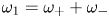 $\omega _1 = \omega _+ + \omega _-$ and
  $\boldsymbol {k}_1 = \boldsymbol {k}_+ + \boldsymbol {k}_-$, where
  $\boldsymbol {k}$ are the wavevectors and the subscripts,
  $1$,
$1$,  $+$ and
  $-$ indicate the primary wave and two resonant waves, respectively. For the
  $A=8 \ \textrm {mm}$ experiment (figure 4b), two lower frequencies (
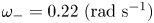 $\omega _- = 0.22\ (\textrm {rad}\ \textrm {s}^{-1})$
  $\omega _+ = 0.33\ (\textrm {rad}\ \textrm {s}^{-1})$) that satisfy the temporal resonant condition are indeed seen to develop, and are maintained throughout the experiment. Moreover, in the
  $A=16\ \textrm {mm}$ case (figure 4c), cascading TRI is observed, where these resonant frequencies in turn become unstable and generate triadic instabilities of their own, seen by further lower frequencies that satisfy the temporal relationship of TRI. These two processes, known as discrete and cascading TRI, have been discussed (case
  $B$ and
  $C$) respectively in Brouzet et al. (Reference Brouzet, Ermanyuk, Joubaud, Sibgatullin and Dauxois2016). As the normalized spectral average over the dissipation scales,
  $\tilde {B}(\omega )/A$, displayed in figure 5 shows, despite the presence of these triadic interactions, the largest congregation of dissipative length scales for all of the forcing amplitudes corresponds to the attractor forcing frequencies, not these resonant frequencies generated from triadic instabilities. Notice instead that high dissipation also takes place at the superharmonic,
  $2 \omega _1$, and at zero frequency. Both result from TWIs that can take place without the need to pass any threshold forcing amplitude. We can therefore identify repeated geometric focusing as the main mechanism for energy dissipation.

Figure 5. Colours present the buoyancy amplitude's spectral decomposition  $\tilde {B}(\omega )/A$ averaged over the dissipation range (from
  $\lambda _1 = 1\ \textrm {cm}$ to
  $\lambda _2 = 2\ \textrm {cm}$, between blue lines in figure 4) and normalized by forcing amplitude
  $A$, as a function of wave frequency and forcing amplitude.
To summarize, the time series of the vertical transects (figure 3k,l) mimic information that one might extract in the ocean from observational records collected with an acoustic Doppler current profiler, thermistor chain or conductivity, temperature and pressure chain. This means that oceanic wave attractors hidden in observational records might be detectable by their increased energy levels at dissipative length scales for attractor frequencies.
3.2. Multiple-frequency forcing
The multi-frequency experiments are forced at 0.5, 1, 2, 4, 8 and 11.5 mm amplitudes with each amplitude containing wave frequencies  $\omega _k = (0.39 + 0.02(k-1))$ for
 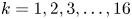 $k=1,2,3,\ldots ,16$, or in short-hand notation
 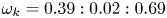 $\omega _k = 0.39:0.02:0.69$. Eight of the input frequencies project into the wave attractor frequency band
  $I_{(1,1)}$, five frequencies are smaller than
  $\omega _{min} =0.477\ \textrm {rad}\ \textrm {s}^{-1}$ and three are larger than
  $\omega _{max} = 0.649\ \textrm {rad}\ \textrm {s}^{-1}$ (see (2.2) for definition). For reproducibility, we chose phases
  $\phi _k$ to be the
  $k\textrm {th}$ digit of
  ${\rm \pi} \approx 3.14159\ldots$ multiplied by
  $2{\rm \pi} /10$, e.g.
  $\phi _3 = 0.4 \times 2 {\rm \pi}$. As mentioned in § 2, the energy input per frequency is found by
  $\omega ^2_k A^2 /K$, meaning we add energy at a strength proportional to
  $\omega ^2_k$.
The snapshots of the weak ( $A = 0.5\ \textrm {mm}$) multi-frequency forcing (figure 6a,c,e,g) depict various diamond-shape (1,1)-attractors. However, the time average of the magnitude of the buoyancy gradient,
  $|\boldsymbol {\nabla } b|$, in figure 6(i) indicates that the sum of the eight excited wave attractors leads to no energy localization. For the large-amplitude regime (
 $A = 8\ \textrm {mm}$), as expected, the wave attractor does not have an obvious appearance for either the snapshots or the time average of the magnitude of the buoyancy gradient (figure 6b,d,f,h and 6j). Specifically, neither of the time series shown in figure 6(k,l) show a clear indication that a wave attractor has formed. Nevertheless, examining the spatio-temporal spectra we find that, as for the series of single-frequency experiments, the wave attractor energy cascade towards the dissipative length scales persists in the presence of a multi-frequency wave field. This is shown in figures 7(a–c) and 8, where the intensified energy levels at attractor frequencies are visible for all forcing amplitudes
  $A$. It should be noted that, while this is less obvious for the highest forcing amplitudes (
 $A = 8\ \textrm {mm}$ and 11.5 mm), the colour scale presented is logarithmic which makes a factor of 2 increase harder to identify.


Unlike the single-frequency forcing, the spectral decompositions of the magnitude of the buoyancy gradient  $|\boldsymbol {\nabla } b|$ in figure 7 do not provide clear evidence of TRI. This comes as no surprise, because the threshold for the onset of TRI depends on the energy per frequency (
 $\propto A^2/K$) rather than the total energy input (
 $\propto A^2$). Hence, the most energetic multi-frequency experiment with
  $A=11.5\ \textrm {mm}$ amplitude forcing corresponds to
  $A = 11.5/\sqrt {16} = 2.87\ \textrm {mm}$ forcing for the single-frequency forcing; for our experiments there has been no TRI observed for
  $A\leq 4\ \textrm {mm}$. It should be noted that this amplitude threshold only exists for finite width beams. Studies by Brouzet (Reference Brouzet2016) and Bourget et al. (Reference Bourget, Scolan, Dauxois, Le Bars, Odier and Joubaud2014) have examined this threshold, considering different beam widths and stratifications, finding amplitude threshold values of a similar magnitude.
While TRI was not observed in the multi-frequency experiments, TWIs were. The frequencies corresponding to these interactions are shown by the black arrows on figure 8, where increased energy levels can be seen at these frequencies. Despite their presence, as with the case of TRI in the single-frequency experiments, the largest congregation of dissipative length scales for all of the forcing amplitudes corresponds to the attractor forcing frequencies, not these TWI frequencies. Moreover, for both the single- and multi-frequency forcing, while normalized energy levels at most wave frequencies increase with increasing forcing amplitude,  $A$ (figures 5 and 8), the most energetic frequencies within the (1,1)-attractor band (between vertical black lines) remain nearly constant. The latter indicates that geometric focusing by the wave attractor (a linear process in
  $A$) is unaltered by nonlinear processes (TRI and TWI).
In the large-amplitude regime, intense overturning took place near the bottom, which created an approximately 5 cm thick homogeneous bottom layer (also contaminated with glycerol entrained from beneath the wavemaker) by the end of the experiment. This intensified bottom mixing might have been driven by barotropic sloshing that was inevitably generated by the peristaltic action of the boundary motion. The homogeneous bottom layer slightly shifted the attractor frequency range  $I_{(1,1)}$ towards larger frequencies, noticeable in figure 7(c) at
  $A = 11.5\ \textrm {mm}$. Interestingly, while larger spatial scales are seen for all small-amplitude, multi-frequency forcing frequencies (figure 7a), we observe a specific frequency within the attractor band that seems to be preferred at dissipative scales. Due to this shift in the attractor range, this corresponds to the frequency in the middle of the attractor range, hence the one least affected by internal shear, as discussed in § 2.
4. Concluding remarks
Our analysis reveals that the projection of wave energy to smaller scales at wave attractor frequencies persists in the large-amplitude single- and multi-frequency regimes. This means that the energy cascade in the ocean can be accelerated by the presence of wave attractors, even if in the presence of (large-amplitude) wave turbulence. We thereby consolidate the general thought (Sibgatullin & Ermanyuk Reference Sibgatullin and Ermanyuk2019) that wave attractors could contribute to the energy cascade towards dissipative scales in the ocean.
Brouzet et al. (Reference Brouzet, Ermanyuk, Joubaud, Sibgatullin and Dauxois2016, Reference Brouzet, Ermanyuk, Joubaud, Pillet and Dauxois2017) and Brunet et al. (Reference Brunet, Dauxois and Cortet2019) emphasized the possibility of single-frequency wave attractors triggering TRI in the large-amplitude regime. Their studies did not indicate whether the occurrence of TRI limited the efficiency of the wave attractor to project energy to the dissipative scales. We show that the linear mechanism of geometric focusing persists in the large-amplitude single-frequency regime, despite the dispersion of wave energy to non-attractor frequencies through TRI and TWIs. Similarly, the wave attractor energy cascade remains efficient if the large-scale energy input consists of multiple frequencies to begin with. We find no evidence of TRI in our multi-frequency experiments, because significant energy content per wave frequency is below the threshold for TRI and possibly due to energy transfer to non-attractor frequencies being generated by TWIs. Time constraints did not allow us to perform an experiment where the forcing frequency or frequencies were all located outside simple attractor frequency bands. We expect that when new frequencies, arising through TRI or TWI, land in one these attractor bands, these may likewise contribute to a rapid transfer to dissipation scales.
Wave attractors have never been observed in ocean records. It is often argued that this is due to the sparsity of observational data. Our analysis shows that hidden wave attractors can be detected from increased energy levels at dissipative scales at the attractor frequencies. For observational records revealing elevated energy levels (as compared to the ‘universal’ GM spectrum) at a specific frequency band, it could be a fruitful exercise to check whether this frequency band corresponds to a family of simple wave attractors in the ocean geometry surrounding the measurement site.
In reality, as briefly mentioned above, the simple attractor frequency bands may not incorporate tidal frequencies at which most oceanic internal waves are generated. In that case, we might expect nonlinear processes to cascade the internal wave energy to attractor frequency bands before the linear process of repeated geometric focusing sets in.
Acknowledgements
We are grateful for the valuable comments by three anonymous referees. We thank the technicians in DAMTP for technical support, T. Dobra for help in writing the code needed to run our experiments with the ASWaM, and C. Brouzet for providing the customized colormap that is used in figures 7 and 8.
Funding
F.B. is grateful for support by NWO Mathematics of Planet Earth grant 657.014.006 and the  $\textrm {NDNS}+$ travel grant that paid for two visits to Cambridge University. KMG is supported by the Natural Environment Research Council (grant number NE/L002507/1).
Declaration of interests
The authors report no conflict of interest.


 Open access