


1. Introduction
Canopy flows are common in the lower part of the atmosphere, and they have been the topic of many reviews (Finnigan Reference Finnigan2000; Barlow & Coceal Reference Barlow and Coceal2009; Fernando Reference Fernando2010; Belcher, Harman & Finnigan Reference Belcher, Harman and Finnigan2012; Nepf Reference Nepf2012; Brunet Reference Brunet2020). Figure 1(a) shows the layered structure of a vegetation canopy flow. It consists of the roughness sublayer, the logarithmic layer and the wake layer. The definition of the roughness sublayer differs from one community to another (Finnigan Reference Finnigan2000; Fernando Reference Fernando2010; Flack & Schultz Reference Flack and Schultz2014; Chung et al. Reference Chung, Hutchins, Schultz and Flack2021; Flack & Chung Reference Flack and Chung2022). Here, the roughness sublayer contains the canopy layer. The behaviour of the mean flow plays an important role in defining the layers in a rough-wall boundary layer. The mean velocity profile in the logarithmic layer follows the logarithmic law of the wall (Raupach & Thom Reference Raupach and Thom1981), and the mean flow in the wake layer abides by Townsend's outer layer similarity (Townsend Reference Townsend1976; Jiménez Reference Jiménez2004). Lastly, Raupach et al.'s mixing-layer analogy gives an estimate of the flow in the canopy sublayer (Raupach, Finnigan & Brunet Reference Raupach, Finnigan and Brunet1989, Reference Raupach, Finnigan and Brunet1996).

Figure 1. (a) A sketch of a vegetation canopy flow. The flow consists of the wake layer, the logarithmic layer and the roughness sublayer. Here,  $\delta$ is the height of the boundary layer above the canopy, $h$ is the height of the canopy and $U_h$ is the velocity (wind speed) at the top of the canopy. The inflected velocity profile in the roughness sublayer gives rise to K–H-type waves above the canopy. (b) A sketch of a plane mixing layer. The inflected velocity profile gives rise to K–H instability. Here, ${\rm \Delta} U$ is the velocity difference between the two streams. A vertical ( $z$) coordinate is defined such that the origin is at the top of the canopy, which corresponds to the centre of the mixing layer. The flow is symmetric with respect to $z=0$.
1.1. Mixing-layer analogy and vegetation canopy flows
First, we explain what the mixing-layer analogy is. Raupach et al. (Reference Raupach, Finnigan and Brunet1989) noticed that the inflected velocity profile in the roughness sublayer is similar to that in a plane mixing layer and hypothesized that the roughness sublayer is analogous to a plane mixing layer. This hypothesis was elaborated in Raupach et al. (Reference Raupach, Finnigan and Brunet1996), according to which the inflected velocity profile in the roughness sublayer gives rise to two-dimensional Kelvin–Helmholtz (K–H) waves.
An extensive review of the mixing-layer literature and the K–H instability falls outside the scope of this work, but a summary of the basics helps the discussion that follows. Consider a plane mixing layer, as sketched in figure 1(b). The inflected velocity gives rise to a shear length scale
 \begin{equation} L_{s,ML}=\frac{{\rm \Delta} U/2}{{{{\rm d}}U}/{{{\rm d}}z}|_{z=0}}, \end{equation}
where  ${\rm \Delta} U$ is the velocity difference between the two streams. The factor 2 is included here to simplify the derivations in the following sections. Linear stability analysis gives an estimate of K–H waves’ spacing, i.e. $\varLambda _x=7L_s$ to $10L_s$.
Now, we consider the canopy flow. The velocity profile in the roughness sublayer is also inflected and should give rise to a similar shear length scale
 \begin{equation} L_s=\left.\frac{U}{{{{\rm d}}U}/{{{\rm d}}z}}\right|_{z=0}, \end{equation}
and the spacing of the transverse vortices in the roughness sublayer should be  $\varLambda _x=7L_s$ to $10L_s$. Raupach et al. (Reference Raupach, Finnigan and Brunet1996) measured vertical velocity correlations in a number of canopy flows and concluded that
 \begin{equation} \varLambda_x=8.1L_s.\end{equation}
Equation (1.3) was found to work well in Novak et al. (Reference Novak, Warland, Orchansky, Ketler and Green2000), Dupont & Brunet (Reference Dupont and Brunet2008), Dupont & Patton (Reference Dupont and Patton2012), Huang, Cassiani & Albertson (Reference Huang, Cassiani and Albertson2009), Bailey & Stoll (Reference Bailey and Stoll2013) and Gavrilov et al. (Reference Gavrilov, Morvan, Accary and Lyubimov Méradji2013) (to name a few) for homogeneous dense vegetation canopies, and is the cornerstone of the mixing-layer analogy. Raupach et al.'s mixing-layer analogy is also evidenced by similar flow structures in other boundary-layer flows and mixing layers (Finnigan Reference Finnigan2000; Finnigan, Shaw & Patton Reference Finnigan, Shaw and Patton2009; Huang et al. Reference Huang, Cassiani and Albertson2009).
Deviations from (1.3) are found in stably stratified canopy flows (Brunet & Irvine Reference Brunet and Irvine2000), in non-homogeneous canopies (Thomas & Foken Reference Thomas and Foken2007), in crop canopies (Py, de Langre & Moulia Reference Py, de Langre and Moulia2006; Dupont et al. Reference Dupont, Gosselin, PY, de Langre, Hemon and Brunet2010; Tschisgale et al. Reference Tschisgale, Löhrer, Meller and Fröhlich2021) and in sparse canopies (Novak et al. Reference Novak, Warland, Orchansky, Ketler and Green2000; Huang et al. Reference Huang, Cassiani and Albertson2009), where the flow is akin to a surface layer rather than a mixing layer. However, these deviations are not unexpected since the mixing-layer analogy is not meant for these flows.
1.2. Mixing-layer analogy and urban-canopy flows
While the vegetation canopy flow community has actively scrutinized the mixing-layer analogy, the urban-canopy flow community has not given nearly as much attention to Raupach et al. (Reference Raupach, Finnigan and Brunet1996). This is partly because the mixing-layer analogy is meant for deep homogeneous canopies, but deep urban canopies are not common and are found only in metropolitan areas (Barlow & Coceal Reference Barlow and Coceal2009). Figure 2 is a sketch of a deep homogeneous urban-canopy flow. Surface roughnesses in an urban canopy are buildings, which are modelled as rectangular prisms. Comparing figures 1(a) and 2, we see that a homogeneous deep vegetation canopy flow and a homogeneous deep urban-canopy flows share a lot in common. They both have a wake layer and a logarithmic layer above the roughness sublayer. Moreover, they both have an inflected mean velocity within the roughness sublayer. It would seem that Raupach et al.'s mixing layer analogy would work well for the flow in urban-canopy flows.

Figure 2. A sketch of an urban-canopy flow. The flow consists of the wake layer, the logarithmic layer and the roughness sublayer. The roughness sublayer contains the canopy occupied region.
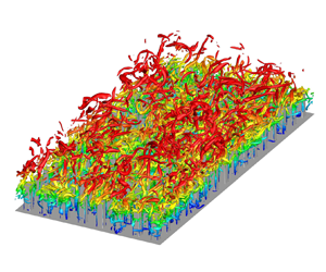
However, Raupach et al.'s mixing-layer analogy has not seen much success in the urban canopy flows. In the following, we explain why. Consider the urban canopy in figure 2. Coceal et al. (Reference Coceal, Dobre, Thomas and Belcher2007) argued that the inflection in the velocity profile at the top of the canopy is a result of the no-slip condition at the top surface of each individual rectangular prism rather than the roughness canopy as a whole. Coceal et al. (Reference Coceal, Dobre, Thomas and Belcher2007) further argued that, in an urban canopy, mixing layers are only found locally, and there are no large-scale K–H waves in urban-canopy flows. Coceal et al.'s (Reference Coceal, Dobre, Thomas and Belcher2007) argument is supported by the available empirical evidence. Huq et al. (Reference Huq, Carrillo, White, Redondo, Dharmavaram and Hanna2007) searched their experimental data but could not find K–H rollers despite extensive visualization attempts. Figure 3 shows the instantaneous vortical structures in a few urban canopies flows obtained from direct numerical simulations. The flow configuration is a half-channel, and the canopy consists of rectangular prisms with the aspect ratio  $h/w_r=4$, where $h$ and $w_r$ are the height and width of the prisms, respectively. The ground coverage density is $\lambda _p=0.06$, 0.11, 0.25 and 0.39 in figure 3(a–d), covering a large range of $\lambda _p$ values. Like the previous authors (Kanda, Moriwaki & Kasamatsu Reference Kanda, Moriwaki and Kasamatsu2004), we cannot find large-scale K–H waves. This becomes more clear if we compare figures 4 and 5, where we show the premultiplied spectra in a canopy flow and a plane channel flow. The two spectra look very much alike, and there is no energy accumulation at any specific wavelength, particularly at the wavelength that corresponds to K–H instability. It is worth mentioning that we choose to show the results in figures 3 and 4 here rather than in the result section because of the following. First, the results in figures 3 and 4 explain the difficulty of Raupach et al.'s mixing-layer analogy in urban-canopy flows and motivate the present work. Second, similar results like the ones in figures 3 and 4 are already extensively available in the present literature and should not need much explanation.

Figure 3. Visualization of instantaneous vortical structures in urban-canopy flows. Shown here are  $Q$ iso-surfaces (Hunt, Wray & Moin Reference Hunt, Wray and Moin1988) coloured by their distances from the ground. The roughnesses are rectangular prisms, whose dimensions are ${w_r} \times {w_r}\times 4{w_r}$. Here, the vertical coordinate is such that the origin is at the ground. The surface coverage densities are (a) $\lambda _p=0.06$, (b) $\lambda _p=0.11$, (c) $\lambda _p=0.25$ and (d) $\lambda _p=0.39$. The flows correspond to R3L06/11/25/39A (see § 4 for details of the direct numerical simulations).

Figure 4. Premultiplied energy spectra of the vertical velocity, i.e.  $k_xk_yE_{ww}$ at a distance $z^{+}=15$ from the canopy crest. The results in panels (a–d) correspond to the flows in figure 3(a–d).

Figure 5. Premultiplied vertical velocity energy spectra, i.e.  $k_xk_yE_{ww}$ in plane channel flow of $Re_{\tau }=550$ (where the friction Reynolds number $Re_\tau$ is defined based on the friction velocity and the half channel height) at $z^{+}=60$ above the wall. Figure reproduced using data reported in del Alamo et al. (Reference del Alamo, Jimenez, Zandonade and Moser2004).
Although (1.3) does not hold for homogeneous urban-canopy flows, we cannot hasten to the conclusion that Raupach et al.'s mixing-layer analogy fails. Here, we explain why. We begin by reviewing the historical background of Raupach et al. (Reference Raupach, Finnigan and Brunet1989) and Raupach et al. (Reference Raupach, Finnigan and Brunet1996). Before the establishment of the mixing-layer analogy, the conventional view was that the roughness sublayer of a vegetation canopy is a superposition of standard surface layer and small-scale turbulence generated in the wakes of plant elements (Raupach & Thom Reference Raupach and Thom1981). In the 1970s, it becomes evident that this view is false. For one, the velocity profile is inflected. For another, the velocity in the roughness sublayer is controlled by a single length scale rather than many scales as in a surface layer. The mixing-layer analogy was proposed in the 1980s to account for these facts. Raupach et al. (Reference Raupach, Finnigan and Brunet1996) put an emphasis on (1.3), but the foundations of the mixing layer analogy are the inflected velocity and the single length scale in the canopy layer, both of which show their presence in homogeneous deep urban-canopy flows. Following this logic, the mixing layer analogy should apply to urban-canopy flows. The challenge, however, is to find mathematical formulations one can put to the test.
1.3. This work
The objective of the present work is to find mathematical formulations that one can test to confirm/refute the mixing-layer analogy and then put these formulations to the test in direct numerical simulations (DNSs) of urban-canopy flows. DNS resolves all scales in a turbulent flow and is the most accurate computational fluid dynamics tool. A limitation of DNS is its high cost (Yang & Griffin Reference Yang and Griffin2021), and because of its high cost, the use of DNS has been limited to low and moderate Reynolds number flows (Moin & Mahesh Reference Moin and Mahesh1998). Canopy flows in the lower part of the atmosphere are at high Reynolds numbers and are usually studied using wall-modelled large-eddy simulation (WMLES) (Giometto et al. Reference Giometto, Christen, Meneveau, Fang, Krafczyk and Parlange2016; Yang Reference Yang2016b; Zhu et al. Reference Zhu, Iungo, Leonardi and Anderson2017; Zhu & Anderson Reference Zhu and Anderson2018; Fan et al. Reference Fan, Ge, Tan and Li2021; Yang & Ge Reference Yang and Ge2021; Zhang et al. Reference Zhang, Wan, Xia, Wang, Lu and Chen2021a,Reference Zhang, Wan, Xia, Wang, Lu and Chenb). However, a WMLES does not resolve the flow close to the top surfaces of roughness elements and the thin shear layers downstream of the roughness elements, which are critical to the mixing layer analogy.
The discussion so far has focused on topics that are closely registered near the mixing layer analogy, and we have not covered the previous research on homogeneous deep urban canopy. Urban-canopy flow is, in general, a very well-researched topic (Barlow & Coceal Reference Barlow and Coceal2009). Idealized urban canopies have been studied experimentally (Cheng & Castro Reference Cheng and Castro2002; Huq et al. Reference Huq, Carrillo, White, Redondo, Dharmavaram and Hanna2007; Inagaki & Kanda Reference Inagaki and Kanda2008; Hagishima et al. Reference Hagishima, Tanimoto, Nagayama and Meno2009), computationally (Kanda et al. Reference Kanda, Moriwaki and Kasamatsu2004; Coceal et al. Reference Coceal, Thomas, Castro and Belcher2006; Leonardi & Castro Reference Leonardi and Castro2010; Lee, Sung & Krogstad Reference Lee, Sung and Krogstad2011; Anderson, Li & Bou-Zeid Reference Anderson, Li and Bou-Zeid2015b; Cheng & Porté-Agel Reference Cheng and Porté-Agel2015; Li & Bou-Zeid Reference Li and Bou-Zeid2019) and theoretically (Yang et al. Reference Yang, Sadique, Mittal and Meneveau2016; Chung et al. Reference Chung, Hutchins, Schultz and Flack2021). However, the existing studies are, by and large, limited to low aspect ratio roughness elements, and deep canopy flow remains an insufficiently explored territory (Sadique et al. Reference Sadique, Yang, Meneveau and Mittal2017; MacDonald et al. Reference MacDonald, Ooi, García-Mayoral, Hutchins and Chung2018). A more in-depth review of the urban-canopy literature falls outside the scope of this work, but in anticipation of § 2, reviewing the layered structures of the urban-canopy layer would be beneficial. Figure 2 is a sketch of the layered structure of the canopy layer. The roughness elements are rectangular prisms of the same height. The flow in the active layer directly exchanges momentum and energy with the flow above the canopy. The flow in the inactive layer, on the other hand, does not, at least not directly. The flow in figure 2 is pressure driven. The pressure force pushes the flow through the roughness in the inactive layer as in a porous medium. A ground layer emerges between the inactive layer and the ground connecting the finite fluid velocity in the inactive layer to 0 velocity at the ground level. In a zero-pressure-gradient (ZPG) deep canopy flow, the velocity in the inactive layer is 0 because of a lack of a driving force, and the inactive layer and the ground layer become one, as sketched in figure 6(b). Figure 6(c) is a sketch of a shallow urban canopy, where the flow in the canopy is affected by the boundary layer above the canopy as well as the ground. Evidently, the flow in a shallow urban canopy is more akin to a surface layer, where the mixing-layer analogy would not apply. This work focuses on the pressure-driven deep canopy flows, i.e. flow sketched in figure 6(a).

Figure 6. Sketches of urban-canopy flows: (a) pressure-driven deep urban-canopy flow, (b) ZPG deep urban-canopy flow, (c) shallow urban canopy.
The rest of the paper is organized as follows. In § 2, we show that the exponential profile is closely related to Raupach et al.'s mixing-layer analogy. In § 3, we derive mathematical formulations that can be tested to confirm/refute Raupach et al.'s mixing layer analogy. These mathematical formulations are put to the test in § 5 after we detail our DNS set-up in § 4. Further discussion of the results is included in § 6, followed by conclusions in § 7.
2. The exponential profile
In § 3, we will show that the velocity following an exponential scaling in the urban canopy is direct evidence for Raupach et al.'s mixing-layer analogy. In anticipation of § 3, we review Inoue (Reference Inoue1963) and Cionco's (Reference Cionco1965) original formulation of the exponential profile, explain why it has seen limited success (MacDonald Reference MacDonald2000; Yang Reference Yang2016a; Yang et al. Reference Yang, Sadique, Mittal and Meneveau2016) and propose a new formulation.
2.1. Inoue and Cionco's original formulation
We begin by deriving Inoue and Cionco's original formulation. Consider a fully developed atmospheric boundary layer over a deep urban canopy. The momentum equation reads
 \begin{equation} -\frac{{{{\rm d}} \langle \overline{u'w'} \rangle }}{{{{\rm d}}z}} - {C_d}{U^{2}}=0, \end{equation}
in the canopy (Inoue Reference Inoue1963; Cionco Reference Cionco1965), where  $\overline {u'w'}$ is the Reynolds shear stress, and $C_d U^{2}$ is the drag force exerted by the urban roughness. Here and throughout the paper, $u$,
$u$,  $v$ and $w$ are the velocity in the streamwise ( $x$), spanwise ( $z$) and wall-normal ( $z$) directions, respectively, $\bar {{\cdot }}$ denotes time averaging, $\langle {\cdot } \rangle$ denotes comprehensive/superficial averaging in the $x$ and $y$ directions (Mignot, Barthelemy & Hurther Reference Mignot, Barthelemy and Hurther2009; Xie & Fuka Reference Xie and Fuka2018; Schmid et al. Reference Schmid, Lawrence, Parlange and Giometto2019). The averaging includes the solid volume within which the fluid velocity is assumed to be 0. Here, $C_d$ is the drag coefficient (and depends on the canopy layout), and $U=\langle \bar {u} \rangle$ is the double-averaged velocity in the $x$ direction. The mean flow advection, the viscous diffusion and the pressure force are neglected since the flow is fully developed, and is not subjected to any mean pressure gradient at a high Reynolds number. Invoking the eddy viscosity model and mixing length model, we have
 \begin{equation} -\langle \overline{u'w'} \rangle=\nu_t\frac{{{\rm d}}U}{{{\rm d}}z}= \left(l_m^{2}\left|\frac{{{\rm d}}U}{{{\rm d}}z}\right|\right)\frac{{{\rm d}}U}{{{\rm d}}z}, \end{equation}
where  $\nu _t$ is the turbulent viscosity, and $l_m$ is the mixing length and is approximately a constant in the urban canopy (Bai, Meneveau & Katz Reference Bai, Meneveau and Katz2012; Forooghi, Yang & Abkar Reference Forooghi, Yang and Abkar2020). Plugging (2.2) into (2.1), we have
 \begin{equation} \frac{{{\rm d}} }{{{{\rm d}}z}}\left[{\left( {l_m\frac{{{{\rm d}}U}}{{{{\rm d}}z}}} \right)^{2}}\right] = {C_d}{U^{2}}, \end{equation}
and one can easily verify that the following exponential profile is a solution to (2.3)
 \begin{equation} U = U_h \exp\left(a\frac{z}{h}\right)= U_h \exp\left(\frac{z}{L_m}\right). \end{equation}
Here, we put the origin of the  $z$ coordinate at the top of the urban canopy, and the canopy occupies $-h< z<0$, $U_h$ is the velocity at top of the canopy (following the conventional notation), $L_m=h/a$ is the attenuation length scale and $a$ is the attenuation factor.
In the above derivation, Inoue (Reference Inoue1963) and Cionco (Reference Cionco1965) invoked the following assumptions in addition to a constant  $C_d$ and a constant $l_m$. First, the viscous diffusion is negligible. Second, the mixing length $l_m$ is a constant. Third, the flow is not subjected to any mean pressure gradient. The exponential profile will not be valid if any of the above assumptions is not true.
2.2. A few caveats
There are a number of caveats when applying (2.4), which are often ignored (Castro Reference Castro2017). First, (2.4) is meant for ZPG flows and is not valid for pressure-driven flows. To make this clear, let us consider a deep urban canopy, for which  $h\gg L_m$. Let us consider a $z$ location that is sufficiently far away from the canopy crest and also sufficiently far away from the bottom wall, i.e. a $z$ location in the inactive layer. This should be possible if the canopy is deep. There, the vertical momentum flux is small, and according to (2.4), we should have $U=U_h\exp (z/L_m)\approx 0$. However, this is true only if it is a ZPG urban-canopy flow. When the mean pressure gradient is non-zero, the pressure force pushes the fluid through the urban canopy. The moving fluid gives rise to a non-zero drag force, which then balances the driving pressure force, leading to the following Reynolds-averaged momentum equation:
 \begin{equation} - \frac{{{{\rm d}}P}}{{{\rm d}\kern0.7pt x}} = \rho{C_d}{{U_c}^{2}}, \quad -h\ll z\ll 0, \end{equation}
where  $P$ is the double-averaged pressure, and $U_c$ is the non-zero double-averaged velocity in the inactive layer. In light of the discussion above, the exponential profile should really be
 \begin{equation} \frac{U-U_c}{U_h-U_c}=\exp\left(\frac{z}{L_m}\right), \end{equation}
for pressure-driven urban-canopy flows. It is worth noting that (2.6) is a physical ansatz rather than a solution of the governing equation.
The second caveat is: (2.4) is valid only sufficiently far away from the ground, i.e. for  $z$ such that $L_m\ll (z+h)$ (note that $z=0$ at the canopy top and $z=-h$ at the ground). This requirement arises because (2.4) is valid if and only if the mixing length $l_m$ is a constant. Since the ground constrains the mixing length (Townsend Reference Townsend1976; Marusic & Monty Reference Marusic and Monty2019; Yang & Meneveau Reference Yang and Meneveau2019; Zhang et al. Reference Zhang, Wan, Xia, Wang, Lu and Chen2021b), (2.4) fails close to the ground. In a pressure-driven deep canopy boundary layer, a ground layer emerges close to the wall, and the fluid velocity decreases from $U_c$ to $0$ on the ground (Huang et al. Reference Huang, Cassiani and Albertson2009).
The third caveat is: (2.4) is valid only in regions where the viscous term is small. In vegetation canopy flows, this is barely an issue. The viscous term is small except very close to the ground, where (2.4) is not valid anyway. This, however, is not true for rectangular roughness arrays with smooth top surface. The no-slip top surfaces of these rectangular roughness elements give rise to a sharp velocity gradient at the top of the canopy, and viscous diffusion becomes the dominant term in the momentum equation especially when the roughness packing density is sufficiently high (Xu et al. Reference Xu, Altland, Yang and Kunz2021). For these rectangular roughness arrays, the origin of the exponential profile cannot be at the top of the canopy, and a displacement  $d_c$ must be incorporated
 \begin{equation} \frac{U}{U_h}=\exp\left(\frac{z+d_c}{L_m}\right). \end{equation}
2.3. A new formulation
Taking into consideration these caveats in § 2.2, we propose a new formulation for homogeneous deep canopy flows,
 \begin{equation} \frac{U-U_c}{U_h-U_c}=\exp\left(\frac{z+d_c}{L_m}\right), \quad {\rm for}\ L_m\ll(z+h),\ z+d_c<0, \end{equation}
where, again, the coordinate is such that  $z=0$ at the top of the canopy, $U_c$ accounts for a non-zero $-{{\rm d}}P/{{\rm d}\kern0.7pt x}$ and is such that $-\rho C_dU_c^{2}-\rho \, {{\rm d}}P/{{\rm d}\kern0.7pt x}=0$, $U_h$ is the double-averaged velocity at the top of the canopy and is a normalization velocity scale, $d_c$ accounts for the sharp velocity gradient at the top of canopy when the canopy is a rectangular roughness array of the same height and $L_m$ is the attenuation length scale. For a ZPG atmospheric boundary layer over vegetation canopies, $U_c=0$, $d_c\approx 0$, and (2.8) reduces to Inoue and Cionco's original formulation in (2.4). For dense and deep urban canopies, $d_c\approx 0$, $U_c\approx 0$, $z+d_c\approx z$ in most of the exponential layer, and the new formulation (2.8) reduces to Inoue and Cionco's original formulation as well. The new formulation (2.8) contains the following parameters: $U_c$, $d_c$ and $L_m$, and is applicable sufficiently far away from the ground and for $z<-d_c$.
3. Mixing-layer analogy in deep urban-canopy flow
In this section, we derive mathematical relations that can be tested to confirm or refute Raupach et al.'s mixing-layer analogy in the context of deep urban-canopy flows.
In a plane mixing layer, where the velocities of the two streams are  $U_1$ and $U_2$, the velocity follows the universal scaling (Pope Reference Pope2000)
 \begin{equation} \frac{{U - {U_2}}}{{{U_1-U_2}}} = f\left( {\frac{{z}+l}{{{{L_s}}}}} \right), \end{equation}
where  $U_1>U_2$, ${L_s}$ is the shear length scale, $l$ is a displacement length and $f$ is a generic function (Rogers & Moser Reference Rogers and Moser1994). Invoking the mixing-layer analogy, the velocity in the urban canopy should follow a similar scaling. In other words,
 \begin{equation} \frac{{U - {U_c}}}{{{U_h} - {U_c}}} = f \left( {\frac{{z+l}}{{{L_s}}}} \right), \end{equation}
where  $z$ is the vertical coordinate. Comparing the exponential profile in (2.8) and the ansatz in (3.2), we notice that the exponential profile is direct evidence for the mixing-layer analogy: the universal function $f$ in (3.2) is the exponential function $\exp ({\cdot })$ in (2.8), the displacement $l$ is $d$ and $L_s$ is $L_m$.
The most challenging part of applying the exponential profile is  $L_m$. In the following, we estimate $L_m$. To do that, we write the force balance in a canopy flow
 \begin{equation} \int_{{-}h}^{0} \rho{C_d}U{{(z)}^{2}}\, {{\rm d}}z = {-} ({h+\delta}) \frac{{{{\rm d}}p}}{{{\rm d}\kern0.7pt x}}, \end{equation}
where the drag balances the driving pressure force, and we have neglected the skin friction. It is worth noting that (3.3) is a direct consequence of the mean momentum equation and can be obtained by integrating the mean momentum equation from the ground to the top boundary. Plugging (2.6) into (3.3), we have
 \begin{equation} {\left( {\frac{{{U_h}}}{{{U_c}}} - 1} \right)^{2}} \frac{{{L_m}}}{2}\left[ {1 - \exp \left( -{2\frac{{ h}}{{{L_m}}}} \right)} \right] + 2\left( {\frac{{{U_h}}}{{{U_c}}} - 1} \right){L_m}\left[ {1 - \exp \left(-{\frac{{h}}{{{L_m}}}} \right)} \right] = \delta. \end{equation}
In a deep canopy,  $h \gg L_m$, $\exp (-h/L_m)\approx 0$ and (3.4) becomes
 \begin{equation} \frac{1}{2}{\left( {\frac{{{U_h}}}{{{U_c}}} - 1} \right)^{2}}{{L_m}} + 2\left( {\frac{{{U_h}}}{{{U_c}}} - 1} \right){L_m} = \delta. \end{equation}
Rearranging (3.5), we arrive at an estimate of the shear length scale
 \begin{equation} \frac{{{L_m}}}{{\delta}} \approx \frac{2}{{\left( {{U_h}/{U_c} - 1} \right)\left( {{U_h}/{U_c} + 3}\right)}}, \end{equation}
which should be true irrespective of the Reynolds number and other parameters. Plugging in (2.8) into (3.3) gives a longer expression but leads to the same conclusion after simplification as we will show in § 6.2.
Equations (3.2) and (3.6) are mathematical formulations that can be tested to confirm or refute Raupach et al.'s mixing-layer analogy in the context of deep canopy flows.
4. Direct numerical simulation
We conduct DNSs to test (3.2) and (3.6). In this section, we present the details of the DNS set-up. The pseudo-spectral code LESGO is employed for our DNSs. The code solves the incompressible Navier–Stokes equations in a periodic half-channel. It uses a pseudo-spectral method in the streamwise and spanwise directions and a second-order finite difference method in the wall-normal direction. A second-order Adams–Bashforth method is employed for time advancement. The flow is pressure driven. Canopy roughness is resolved using an immersed boundary method (Chester, Meneveau & Parlange Reference Chester, Meneveau and Parlange2007). Many have used this code for boundary-layer flow simulations, including flows over complex terrain (Anderson & Chamecki Reference Anderson and Chamecki2014; Anderson et al. Reference Anderson, Barros, Christensen and Awasthi2015a), vegetative canopies (Chester et al. Reference Chester, Meneveau and Parlange2007; Bai et al. Reference Bai, Meneveau and Katz2012) as well as urban canopies (Cheng & Porté-Agel Reference Cheng and Porté-Agel2015; Giometto et al. Reference Giometto, Christen, Meneveau, Fang, Krafczyk and Parlange2016; Yang et al. Reference Yang, Xu, Huang and Ge2019).
We consider deep canopy flows. The roughnesses are rectangular prisms. Two roughness arrangements are considered, namely, aligned and staggered, as sketched in figure 7(a,b). Here,  $s$ is the spacing of the prisms, and ${w_r}$ is the width of the prisms. In most cases, $h/{w_r}=4$ and $\delta /{w_r}=4$, 6. The spacing $s/{w_r}$ is 1.6, 2, 3, or 4. The surface coverage density, $\lambda _p={w_r}^{2}/s^{2}$, is 0.39, 0.25, 0.11 or 0.06. Figure 7(c) shows a side view of the flow domain.

Figure 7. (a,b) Top views of a repeating tile for the aligned/staggered configuration, (c) side view of the canopy and (d) perspective view of the canopy (here,  $h/{w_r}=4$, $\lambda _p=0.25$).
Similar configurations are considered by Sharma & Garcia-Mayoral (Reference Sharma and Garcia-Mayoral2020) and MacDonald et al. (Reference MacDonald, Ooi, García-Mayoral, Hutchins and Chung2018) in their numerical studies of deep roughness canopies. Figure 7(d) is a perspective view of a specific case, i.e.  $h/{w_r}=4$, $\delta /{w_r}=4$ and $\lambda _p=0.25$.
In addition to the canopy geometry, the flow is controlled by the Reynolds number. The Reynolds number of a deep canopy boundary layer can be defined in a few ways (MacDonald et al. Reference MacDonald, Ooi, García-Mayoral, Hutchins and Chung2018; Xu et al. Reference Xu, Altland, Yang and Kunz2021), and the nominal Reynolds number and the effective Reynolds number are two. The nominal Reynolds number reads
 \begin{equation} Re_{\tau ,N} = \frac{{{u_{\tau ,N}}(\delta + h)}}{\nu}, \end{equation}
where  $u_{\tau,N}=\sqrt {(\delta +h)(-{{\rm d}}P/{{\rm d}\kern0.7pt x})/\rho }$ is the nominal friction velocity, and $\nu$ is the kinematic viscosity. The effective Reynolds number reads
 \begin{equation} Re_{\tau ,E} = \frac{{{u_{\tau ,E}}\delta }}{\nu }, \end{equation}
where  $u_{\tau,E}=\sqrt {\delta (-{{\rm d}}P/{{\rm d}\kern0.7pt x})/\rho }$ is the effective friction velocity. Since the canopy occupies a substantial portion of the computational domain, the nominal Reynolds number will be larger than the effective Reynolds number. Considering that the boundary layer interacts with only the top part of the canopy, the effective Reynolds number is a more appropriate measure of the ratio between the largest and the smallest scales in the flow – although the computational cost scales with the nominal Reynolds number. Three Reynolds numbers are considered, namely $Re_{\tau,E}=280$, 367 and 560. These effective Reynolds numbers correspond to $Re_{\tau,N}=790$, and 1580.
Table 1 shows the details of our DNSs, where we tabulate the effective and the nominal Reynolds numbers, the domain sizes, the canopy and the boundary-layer heights, the grid numbers in the three Cartesian directions and the number of rectangular prisms in the streamwise and the spanwise directions. The nomenclature of the cases is as follows:  $R[Re_{\tau,E}/100]L[100\lambda _p][{A/S}]$, where $A$ is for ‘aligned’ and $S$ is for ‘staggered’. Here and throughout the paper, the superscript ‘ $+$’ denotes normalization by $u_{\tau,E}$ and $\nu /{u_{\tau,E}}$.
Table 1. DNS details. Here,  $L_x$, $L_y$ and $L_z$ are the domain sizes in the streamwise, spanwise and vertical directions, respectively; ${w_r}$ is the width of the prisms; $h$ is the canopy height; $\delta$ is the height of the boundary layer above the canopy; $N_x$, $N_y$ and $N_z$ are the numbers of the grid points in the streamwise, spanwise and vertical directions, respectively; $n_x$ and $n_y$ are the numbers of prisms in the $x$ and $y$ directions. The nomenclature of the cases is as follows: $R[Re_{\tau,E}/100]L[100\lambda _p][{A/S}]$, where A is for ‘aligned’ and S is for ‘staggered’.

Next, we explain our choices of domain size and grid resolution. The boundary layer interacts with only the top part of the canopy, and therefore the height of the boundary layer above the canopy is a more appropriate measure of the domain size than the half-channel height. In our DNSs, the spanwise extents of computational domains are such that  $L_y\ge 4\delta$. The streamwise domain sizes are slightly different for flows at different Reynolds numbers. We use a long streamwise domain for the R3 and R5 DNSs, i.e. $L_x=8\delta$ and $9\delta$, respectively. A shorter streamwise domain is used for the R2 DNSs, i.e. $L_x=4\delta$. In the following, we compare our domains with those in the existing literature. Lozano-Durán & Jiménez (Reference Lozano-Durán and Jiménez2014) studied the effects of domain size on flow statistics and concluded that the streamwise and the spanwise domain sizes must be $L_x>2{\rm \pi} \delta$ and $L_y>3\delta$. The authors argued that a smaller domain might affect the first- and second-order statistics. Lozano-Durán & Jiménez (Reference Lozano-Durán and Jiménez2014) considered plane channel flow. The requirement for canopy flow, or rough-wall channel flow, is different and is less stringent. Leonardi & Castro (Reference Leonardi and Castro2010) used a domain of size $L_x\times L_y\times L_z=8{w_r}\times 6{w_r}\times 6{w_r}$. Coceal et al. (Reference Coceal, Thomas, Castro and Belcher2006) studied the effects of domain size on the flow over cube arrays, and concluded that $L_x\times L_y\times L_z=4{w_r}\times 4{w_r}\times 4{w_r}$ is sufficient if one is interested in only low-order flow statistics. These two domains translate to $L_x\times L_y\times L_z=1.6\delta \times 1.2\delta \times \delta$ and $L_x\times L_y\times L_z=1.33\delta \times 1.33\delta \times \delta$, both of which are notably smaller than the minimum channel in Lozano-Durán & Jiménez (Reference Lozano-Durán and Jiménez2014). In the more recent work, Chung et al. (Reference Chung, Chan, MacDonald, Hutchins and Ooi2015) and MacDonald et al. (Reference MacDonald, Chung, Hutchins, Chan, Ooi and García-Mayoral2017) concluded that, if the purpose is to study the roughness’ aerodynamic properties (which is our purpose), one may well employ a minimal-span channel whose size is $L_y \ge \max (100\nu /u_{\tau },k/0.4,\lambda _{r,y})$, where $k$ is the (effective) roughness height, $\lambda _{r,y}$ is the spanwise length scale of roughness elements. In light of the discussion above and the recent DNS studies (Sharma & Garcia-Mayoral Reference Sharma and Garcia-Mayoral2020), we may conclude that our domains are larger than needed. The purpose of employing a large domain for our higher Reynolds number DNSs is to resolve the K–H waves – if they exist. We have also conducted a DNS where we double the streamwise domain size for R2L11A. The case is referred to as R2L11A(L). In figure 8(a), we compare the mean flows in R2L11A and R2L11A(L), and there is barely any difference. Here and in later sections, all statistics are streamwise and spanwise averaged and temporally averaged for 20 large-eddy turnover times. We can confirm a flow's statistical convergence by examining the momentum budget, which we will do in § 6.4.

Figure 8. The mean velocity profile in R2L11A compared with the results (a) in a larger domain: R2L11A(L), (b) with two coarsened resolutions: R2L11A(M), R2L11A(C) and (c) with two refined resolutions: R2L11A(F1), R2L11A(F2).
In addition, the vertical domain must be sufficiently high so that the top boundary does not affect the flow near the canopy crest. This usually requires the height of the domain above the canopy, denoted as  $\delta$, to be sufficiently larger than the roughness’ characteristic length scale. For deep canopies, the canopy height, denoted as $h$, is not the roughness’ characteristic length scale because the lower part of the canopy does not directly interact with the flow above the canopy. A good measure of the deep canopy's characteristic length scale is the attenuation length scale $L_m$. For the cases studied in this work, $L_m/\delta \lesssim 0.2$, and therefore the top boundary should not affect the flow near the canopy crest. Further evidence will be presented in § 6.3.
Last, we explain our choice of the grid. We use a uniform grid spacing in the streamwise and the spanwise direction and slightly stretch the grid in the wall-normal directions away from the top of the canopy and the ground, where the mean velocity gradient is large. The grid resolution is such that  ${\rm \Delta} x^{+}={\rm \Delta} y^{+}<4.5$ and ${\rm \Delta} z^{+}\approx 2.5$. The wall unit is defined using the kinematic viscosity and the nominal friction velocity $u_\tau =\sqrt {D/\rho }$, where $D$ is the drag force per unit area. In a turbulent rough-wall boundary layer, most drag is form drag, and therefore the defined wall unit is an underestimate (and therefore overly conservative estimate) of the viscous scale at the top of the roughness. A more physical measure of the viscous length scale is the Kolmogorov length scale. Figure 9 shows the grid resolution measured by the Kolmogorov length scale. We see that ${\rm \Delta} x/\eta ={\rm \Delta} y/\eta$ is around 1.5 at most places and nowhere exceeds 2.5, and ${\rm \Delta} z/\eta$ is around 1 at most places and nowhere exceeds 2. This grid resolution is quite high, and we see no apparent Gibbs oscillations in our DNSs. The non-physical Gibbs oscillation has a less significant impact on the simulations with DNS or wall-resolved large-eddy simulation (LES) rather than WMLES, since the velocity in DNS and wall-resolved LES transitions more gradually to the no-slip condition near the wall (Li, Bou-Zeid & Anderson Reference Li, Bou-Zeid and Anderson2016).

Figure 9. Ratio of the grid spacing to the Kolmogorov scale: (a–c)  ${\rm \Delta} x/\eta$, (d–f) ${\rm \Delta} z/\eta$, and (a,d) R2L06/11/25/39A/S, (b,e) R3L06/11/25/39A/S, (c,f) R5L11/25A/S. The solid/dashed lines represent the aligned/staggered configurations respectively.
We also conduct a grid convergence study. Specifically, we coarsen R2L11A's grid by a factor of 1.25 and 1.67 in the horizontal directions. The two cases are R2L11A(M) and R2L11A(C), where M stands for medium and C stands for coarse. Furthermore, we refine R2L11A's grid by a factor 1.5 in the streamwise and the spanwise direction, and stretch the wall-normal grid such that the wall-normal grid resolution at the roughness crest is refined by a factor of 1.25 and 3. These two cases are R2L11A(F1) and R2L11A(F2). We compare the mean flow results in these five calculations in figure 8(b,c). R2L11A(C) yields a slightly lower  $U$ near the top boundary, but the profiles in R2L11A and R2L11A(M) collapse. The R2L11A(F1), R2L11A(F2) and the R2L11A results collapse. These results suggest that the standard grid resolution, i.e. the grid resolution used for R2L11A, is sufficiently fine. It is, however, worth noting that this conclusion applies only to low-order statistics, high-order statistics may well require finer grid resolution (Yang et al. Reference Yang, Hong, Lee and Huang2021). We now compare our grid resolution with those in the literature. The typical grid resolution requirement for flat-plate boundary-layer flow is ${\rm \Delta} x^{+} \approx 12$, ${\rm \Delta} y^{+} \approx 6$, and ${\rm \Delta} z_{max}^{+} \approx 8$ (Kim, Moin & Moser Reference Kim, Moin and Moser1987; Lee et al. Reference Lee, Sung and Krogstad2011; Lozano-Durán & Jiménez Reference Lozano-Durán and Jiménez2014; Xu et al. Reference Xu, Altland, Yang and Kunz2021). The grid resolution requirement for rough-wall boundary layers is similar. The resolution is ${\rm \Delta} x^{+}={\rm \Delta} y^{+}=19$ in Leonardi & Castro (Reference Leonardi and Castro2010), ${\rm \Delta} ^{+}=$7.8 to 15.6 in Coceal et al. (Reference Coceal, Thomas, Castro and Belcher2006) and ${\rm \Delta} z_{max}^{+}=8$ to 13 in MacDonald et al. (Reference MacDonald, Ooi, García-Mayoral, Hutchins and Chung2018). Compared with these previous studies, our grid resolutions are excessive. The purpose of employing such a fine grid resolution is to fully resolve the thin shear layer at the top of the canopy.
5. Evidence for the mixing-layer analogy in deep canopy flows
The basis of Raupach et al.'s mixing-layer analogy is the inflected velocity profile. Figure 10 shows the time- and plane-averaged streamwise velocity in our DNSs. We see that the velocity profiles are inflected at the canopy crest. Although this is trivial, the results in figure 10 is the first evidence for the mixing-layer analogy. In addition to the fact that velocity profiles are inflected, we make the following observations. Firstly, an inactive layer emerges below the active layer (see figure 6 for the definition of the inactive layer), where the mean velocity is approximately constant and equals  $U_c$. The fact that an inactive layer emerges shows that the canopies are deep (Poggi et al. Reference Poggi, Porporato, Ridolfi, Albertson and Katul2004; Nepf Reference Nepf2012; Nikora, Nikora & O'Donoghue Reference Nikora, Nikora and O'Donoghue2013). Secondly, as more roughness leads to more resistance in the canopy layer, $U_c$ decreases as the surface coverage density increases for a given roughness arrangement. Also, as the staggered arrangement leads to more blockage than the aligned arrangement, the staggered arrangement results in a smaller $U_c$ than the aligned arrangement for a given surface coverage density. Thirdly, the reader may notice that the velocity at the top of the half-channel, $U(\delta )/U_h$, is larger in the staggered cases than in the aligned cases. This counter-intuitive result is due to smaller $U_h^{+}$ in the staggered cases: although $U(\delta )^{+}$ is also smaller in the staggered cases, an even smaller $U_h^{+}$ results in a larger $U(\delta )/U_h$ in the staggered cases.

Figure 10. Time- and plane-averaged streamwise velocity profiles. (a) R2 cases, (b) R3 cases, (c) R5 cases. The solid and dashed lines are the aligned and staggered configuration results, respectively. The ranges of the  $x$ and $y$ axes are kept the same among the three figures.
In addition to the inflected velocity profile, (2.8), if confirmed, is evidence for the mixing-layer analogy. In the following, we compare the velocity profile in the canopy layer with (2.8). Figure 11 shows the double-averaged velocity in the canopy layer. The velocity is scaled according to  $(U-U_c)/(U_h-U_c)$, where $U_c$ is the velocity in the inactive layer and is readily available in the DNSs. We see that $\log ((U-U_c)/(U_h-U_c))\sim z/{w_r}$ in the active layer, which is encouraging. In addition, we observe the following. Firstly, the staggered arrangement results in more attenuated velocity profiles than the aligned arrangement for a given surface coverage density. Secondly, the velocity overshoots near the wall. This overshoot is quite peculiar and does not seem to have been reported by any other authors before. However, since this paper does not concern the ground layer, we will leave this overshoot for future investigation.

Figure 11. Mean velocity profiles in the canopy layer. (a) R2 case, (b) R3 cases, (c) R5 cases. Again, the solid and dashed lines represent the aligned and staggered cases.
Next, we fit for  $L_m$ and $d_c$ in the active layer. Figure 12 shows the scaled velocity as a function of $(z+d_c)/L_m$. We see that the mean velocity follows the exponential profile closely from approximately $z+d_c=-2L_m$ to $z+d_c=-0.4L_m$. The extent of the active layer varies from one case to another as the sizes of the viscous layer and the ground layer vary from one case to another. The viscous layer occupies more space at higher packing densities, and the ground layer is thicker at lower packing densities. It is also worth noting that the Reynolds number does not play an important role here, and (3.2) and (3.6) are valid irrespective of the Reynolds number. It is worth noting that whether DNS results are Reynolds number independent is not a concern to us. Our concern is whether (3.2) and (3.6) are valid at all (turbulent) Reynolds numbers. The results in figure 12 is the second evidence for the mixing-layer analogy.

Figure 13 compares the data with (3.6). The range of  $(U_h/U_c-1)(U_h/U_c+3)$ is more than a decade. A higher surface coverage density leads to a larger $U_h/U_c$, which, in turn, leads to a larger $(U_h/U_c-1)(U_h/U_c+3)$. For a given surface coverage density, the staggered arrangement leads to a larger $U_h/U_c$ and a larger $(U_h/U_c-1)(U_h/U_c+3)$ than the aligned arrangement. The data follow (3.6) closely for $(U_h/U_c-1)(U_h/U_c+3)>6$, and the result is the third piece of evidence for the mixing-layer analogy. Disagreements are found for $(U_h/U_c-1)(U_h/U_c+3)<5$, specifically, for $R2L06A/S$ and $R3L06A/S$. In these L06 cases, the active layer intrudes to the wall, and the deep canopy assumption breaks.

Figure 13. The attenuation length scale as a function of  $(U_h/U_c-1)(U_h/U_c+3)$. We use different colours for different Reynolds numbers, i.e. blue for R2, red for R3 and yellow for R5. The open and solid symbols represent aligned and staggered roughness arrangements, with squares for L06A/S, circles for L11A/S, left triangle for L25A/S and right triangle for L39A/S.
6. Discussion
Having presented evidence for the mixing-layer analogy, we now scrutinize some of the claims in the previous sections. In § 6.1, we will explain why (1.3) fails. In § 6.2, we discuss a few extensions of the derivation in § 3. We will show that the canopies in our DNSs are deep in § 6.3 and that our data are statistically converged in § 6.4 . Our results are compared with those in the vegetation canopy flow literature in § 6.5. Last, we will report the roughness properties in § 6.6.
6.1. Revisiting the methodology in Raupach et al. (Reference Raupach, Finnigan and Brunet1996)
We follow Raupach et al. (Reference Raupach, Finnigan and Brunet1996) and compare our data with (1.3). The results will add to the discussion in § 1 and serve as a motivation for the present work.
Raupach et al. (Reference Raupach, Finnigan and Brunet1996) argued that the vertical velocity is less susceptible to inactive eddies and therefore is more indicative of the active eddies in the roughness sublayer than the streamwise component. We follow the previous authors and examine the vertical velocity. Figures 14 and 15 show the contours of the instantaneous vertical velocity fluctuations at  $z^{+}=5$ and $z^{+}=15$, respectively, in the R3 cases. The results in the R2 and R5 cases are similar and are not shown here for brevity. Both $z^{+}=5$ and 15 are within the roughness layer, but the wakes behind the individual roughness elements are less discernible at $z^{+}=15$ than at $z^{+}=5$. To prevent any interplay between the wake flow and the K–H type waves (if they exist), we focus on the data at $z^{+}=15$. There, we see no clear evidence for K–H-type instability, i.e. no K–H rollers.

Figure 14. Contours of the instantaneous vertical velocity fluctuation at  $z^{+}=5$. The shear length scales are indicated above each panel. (a) R3L06A, (b) R3L11A, (c) R3L25A, (d) R3L39A.

Figure 15. Same as figure 14 but for  $z^{+}=15$.
Next, we follow Raupach et al. (Reference Raupach, Finnigan and Brunet1996) and examine the velocity correlation. The two-point correlation reads
 \begin{equation} {R_{\phi_1\phi_2}(z,{z_{ref}},{r_x})} = \frac{{\langle {\phi_1' (x,y,{z_{ref}},t)\phi_2'(x + {r_x},y,z,t)} \rangle }}{{\sqrt {\langle {\phi_1'{{(x,y,{z_{ref}},t)}^{2}}} \rangle \langle {\phi_2'{{(x,y,z,t)}^{2}}} \rangle }}}, \end{equation}
where  $z_{ref}$ is the reference vertical location, $r_x$ is the streamwise separation distance, $\phi '$ is the velocity fluctuation in time. Here, $z_{ref}^{+}=15$. Figures 16 and 17 show the two-point correlation of the streamwise and the vertical velocities, i.e. $R_{uu}$ and $R_{ww}$, in the R3 cases. The statistical object $R_{uu}$ is included here for comparison purposes. We see from figure 16 that the contour lines are inclined towards the positive $x$ direction (Adrian, Meinhart & Tomkins Reference Adrian, Meinhart and Tomkins2000; Heisel et al. Reference Heisel, Dasari, Liu, Hong, Coletti and Guala2018; Zhang et al. Reference Zhang, Wan, Xia, Wang, Lu and Chen2021b). Raupach et al. (Reference Raupach, Finnigan and Brunet1996) measured the spacing between two adjacent eddies in the roughness sublayer according to
 \begin{equation} {\varLambda _x} = 2{\rm \pi} \alpha {L_w}. \end{equation}
Here,  $\alpha =1.8$ is a constant, and $L_w$ is the correlation length scale computed as follows:
 \begin{equation} L_{w}(z_{ref},z) = \int_0^{\infty} {R_{ww}({r_x},{z_{ref}},z)} \,{{\rm d}}{r_x}. \end{equation}
Because of the finite computational domain,  $r_x$ is limited to $L_x/2$, and we employ the following equation for $L_w$:
 \begin{equation} L_{w}(z_{ref}^{+},z) = \frac{1}{2}\int_{{-}L_x/2}^{L_x/2} {R_{ww}({r_x},{z_{ref}^{+}},z)} \, {{\rm d}} {r_x}, \end{equation}
again,  $z_{ref}^{+}=15$. Figure 18 shows the correlation length scale $\varLambda _x$ as a function of the shear length scale $L_s$. We see that the data do not support (1.3) or the presence of K–H rollers. We also examined the data reported in Coceal et al. (Reference Coceal, Dobre, Thomas and Belcher2007), Kanda et al. (Reference Kanda, Moriwaki and Kasamatsu2004), Yang et al. (Reference Yang, Xu, Huang and Ge2019) and Xu et al. (Reference Xu, Altland, Yang and Kunz2021), but could not find K–H rollers. Huq et al. (Reference Huq, Carrillo, White, Redondo, Dharmavaram and Hanna2007) carried out extensive visualization attempts in experiments, and they could not find K–H rollers either. The above is consistent with the existing literature: there are no K–H rollers in urban-canopy flows. Although we cannot exclude the existence of K–H rollers in deep canopy flows, the chance that K–H rollers can be found in deep urban-canopy flows is slim. Following this line of thinking, it would be even harder to find K–H rollers in shallow urban canopies and above closely packed buildings of the same height. The mixing-layer analogy is not meant for the former, and the surface layer analogy is more appropriate for the latter.

Figure 16. Contours of the two-point correlation of the streamwise velocity ( $R_{uu}$) in streamwise/vertical plane. The reference location is at $z_{ref}^{+}=15$, i.e. slightly above the roughness canopy. (a) R3L06A, (b) R3L11A, (c) R3L25A, (d) R3L39A.

Figure 17. Same as figure 16 but for the two-point correlation of the vertical velocity ( $R_{ww}$).

Figure 18. The correlation length scale  $\varLambda _x$ as a function of the shear length scale $L_s$. The solid line represents $\varLambda _x=8.1L_s$, while the horizontal dashed line represents $\varLambda _x/{w_r}=0.7$. The symbols are results obtained from R3 cases (square: R3L06A, circle: R3L11A, left triangle: R3L25A, right triangle: R3L39A).
We remark on the results in this subsection. Firstly, the failure of (1.3) in deep urban-canopy flows and the success of the mixing-layer analogy in deep vegetation canopy flows motivated this work. Secondly, the failure of (1.3) does not invalidate the mixing-layer analogy. Raupach et al. proposed the mixing-layer analogy as an alternative to the surface layer analogy. The analogy has value because it gives us more insights into the flow in the roughness sublayer than the surface layer analogy. While (1.3) has been the cornerstone of the mixing-layer analogy, the analogy is more than (1.3) (Brunet Reference Brunet2020). Thirdly, the failure of (1.3) does not invalidate the arguments that led to it. Raupach et al. argued that the inflected velocity profile would give rise to K–H instability, which then results in (1.3). The velocity profile is an inflected one in urban-canopy flows, and K–H instability surely plays a role in urban-canopy flows (Brunet Reference Brunet2020). Equation (1.3) fails because K–H instability is not the dominant mechanism in deep urban-canopy flows. Fourthly, the failure of (1.3) does not invalidate the shear length scale  $L_s$ or the correlation length scale $\varLambda _x$ as important length scales in the roughness sublayer. The correlation length scale is a measure of the largest eddy in the flow and is undoubtedly an important length scale. Figure 19 compares the shear length scale $L_s$ and the attenuation length scale $L_m$. We see that the two are well correlated.

Figure 19. The shear length scale  $L_s$ as a function of the attenuation length scale $L_m$. We use different colours for different Reynolds numbers: blue for R2, red for R3 and yellow for R5. The open and solid symbols represent the aligned and staggered configurations. Different symbols represent different surface coverage densities. Here, squares: L06A/S, circles: L11A/S, left triangles: L25A/S, right triangles: L39A/S. The solid and dashed lines represent $L_s=0.7L_m\pm 0.05\delta$.
6.2. Further discussion on the formulation in § 3
We discuss two extensions of the derivation in § 3.
Firstly, we consider the limit  $U_c\to 0$. This limit is attained if the buildings are very closely packed or if the boundary-layer flow is not driven by a pressure gradient. At this limit, the velocity in the canopy layer is $U/{U_h} = \exp (z/{L_m})$, i.e. (2.4), and the force balance reads
 \begin{equation} \int_{ - h}^{0} {\rho {C_d}U{{(z)}^{2}}\, {{\rm d}}z} = \rho {u_\tau }^{2}, \end{equation}
with  $u_\tau =\sqrt {\tau _w/\rho }$ by definition. Plugging (2.4) into (6.5) leads to
 \begin{equation} {C_d}{U_h}^{2}\frac{{{L_m}}}{2}[ {1 - \exp ( - 2h/{L_m})} ] = {u_\tau }^{2}. \end{equation}
In a deep canopy, we have  $h \gg L_m$, $\exp (-h/L_m)\approx 0$, and therefore (6.6) becomes
 \begin{equation} {L_m} \approx \frac{2}{{{C_d}{{( {{U_h}/{u_\tau }} )}^{2}}}}, \end{equation}
which suggests that  $L_m$ is inversely proportional to ${( {{U_h}/{u_\tau }} )^{2}}$.
Secondly, we discuss the case if we had plugged (2.8) instead of (2.6) into (3.3). Plugging (2.8) into (3.3), the integration becomes
 \begin{align} &{\left( {\frac{{{U_h}}}{{{U_c}}} - 1} \right)^{2}} \frac{{{L_m}}}{2}\exp \left({\frac{{2{d_c}}}{{{L_m}}}} \right) \left[ {1 - \exp \left( { - \frac{{2h}}{{{L_m}}}} \right)} \right] \nonumber\\ &\quad + 2\left( {\frac{{{U_h}}}{{{U_c}}} - 1} \right){L_m}\exp \left( {\frac{{{d_c}}}{{{L_m}}}} \right)\left[ {1 - \exp \left( { - \frac{h}{{{L_m}}}} \right)} \right] = \delta. \end{align}
Here,  $d_c$ measures the size of the viscous layer at the top of the canopy and is much smaller than $L_m$. It follows that $\exp ({d_c}/{L_m})\approx 1$ and (6.8) reduces to (3.4).
6.3. Canopy depth
A canopy is considered deep if the bottom wall does not affect the flow near and above the canopy crest.
Consider R2L11A(h1), R2L11A(h2), R2L1A (the last case is the standard case where  $h/{w_r}=4$) and R2L11A(h6), where we vary the canopy depth from $h={w_r}$ to $h=6{w_r}$. Figure 20(a,b) shows the comprehensive/superficial average (Mignot et al. Reference Mignot, Barthelemy and Hurther2009; Xie & Fuka Reference Xie and Fuka2018; Schmid et al. Reference Schmid, Lawrence, Parlange and Giometto2019) of the velocity within and above the canopy. The R2L11A and the R2L11A(h6) results collapse in figure 20(a). All four profiles collapse near the canopy crest in figure 20(b). In addition to the velocity profiles, we may examine the roughness properties. Figure 21 shows the roughness function ${\rm \Delta} U^{+}$ and the location of the virtual wall $d/w$, as a function of the canopy depth. The general expectation is as follows (MacDonald et al. Reference MacDonald, Ooi, García-Mayoral, Hutchins and Chung2018). When the canopy is shallow, increasing the canopy depth increases the drag, which in turn increases the roughness function. Meanwhile, increasing the canopy depth pushes the virtual ground away from the canopy crest, and the roughness transitions from k-type to d-type (Jiménez Reference Jiménez2004). Once the roughness is d-type, further increasing the canopy depth has no effect on the roughness function nor the location of the virtual ground as the boundary layer only interacts with the top part of the roughness. We see that ${\rm \Delta} U^{+}$ and $d$ increases as $h$ increases and stay a constant as $h$ increases beyond $h=4w$. Hence, we can conclude that the canopy in R2L11A is a deep one.

Figure 20. The time- and plane-averaged streamwise velocity profile (a) above the canopy and (b) within the canopy for  $h/{w_r}=1, 2, 4$ and 6.

Figure 21. (a) The roughness function and (b) the location of the virtual wall in R2L11A and R2L11A(h1/h2/h6). We will explain how we measure  ${\rm \Delta} U^{+}$ and $d$ in § 6.6.
The canopy in R2L11A is a deep one. This readily guarantees that the canopies are deep in the L11S cases (for R2, R3 and R5), the L25 cases (for R2, R3 and R5, for S and A) and the L39 cases (for R2, R3 and R5, for S and A) because of the following. A canopy is deep if  $h\gtrsim L_m$; $L_m$ is a decreasing function of the surface coverage density, is larger for aligned roughness than for staggered roughness and is insensitive to the Reynolds number (at least for the Reynolds numbers investigated here). Hence, the fact that the canopy in R2L11A is deep ensures the canopies with higher surface coverage densities, higher Reynolds numbers and staggered roughness arrangement are all deep canopies. Nonetheless, it is worth noting that the deep canopy in R2L11A does not guarantee the canopies in the L06 cases are deep, which may well explain the discrepancies between the L06 data and our theory in figure 13.
6.4. Statistical convergence
The Reynolds-averaged  $x$-momentum equation reads
 \begin{equation} \frac{{\rm d}}{{{\rm d}}z}\left(\nu\frac{{\rm d} \langle {U} \rangle}{{{\rm d}}z}-\langle \overline{u'v'} \rangle-\langle u''v'' \rangle\right)-\frac{1}{\rho} \frac{{\rm d} \langle \bar{p} \rangle}{{\rm d}\kern0.7pt x}-f=0, \end{equation}
where  $f$ is the drag force (which is 0 outside the roughness occupied region), ${\rm d}/{{\rm d}\kern0.7pt x}$ and $d/dz$ are total derivative in the $x$ and $z$ directions, respectively (streamwise- and spanwise-averaged velocity and stresses are only functions of $z$),
$z$),  $\nu$ is the kinematic viscosity, $p$ is the pressure, $\bar {{\cdot }}$ denotes time average, $\langle {\cdot } \rangle$ denotes spatial average, $\phi '=\phi - \bar {\phi }$ is the turbulent fluctuation, $\phi ''=\bar {\phi }-\langle \bar {\phi } \rangle$ is the spatial variation and $\phi$ is a generic variable (note that $\overline {\phi ''_i\phi ''_j}\equiv \phi ''_i\phi ''_j$ for any $\phi _i$ and $\phi _j$). The terms on the left-hand side are the viscous diffusion term, the turbulent transport term, the dispersive stress term and the pressure-gradient term. Integrating (6.9) in the $z$ direction leads to
 \begin{equation} \nu\frac{{{\rm d}} \langle {U} \rangle}{{\rm d} y}-\langle \overline{u'v'} \rangle-\langle u''v'' \rangle={\rm Const.}+\frac{1}{\rho}\frac{{{\rm d}} \langle \bar{p} \rangle}{{\rm d}\kern0.7pt x} z, \end{equation}
outside the canopy. The total stress is a linear function of  $z$ if the flow is statistically converged. Equation (6.10) is often used to check the statistical convergence of a numerical simulation: a simulation is statistically converged if the sum of the viscous, turbulent and dispersive fluxes is a linear function of $z$ (Oliver et al. Reference Oliver, Malaya, Ulerich and Moser2014). Figure 22 shows the terms in (6.10) in the R3 cases. The results in the R2 and R5 cases are similar and are not shown here for brevity. The total stress is a linear function of $z$, and therefore the flow is statistically converged.

Figure 22. The terms in the Reynolds-averaged  $x$-momentum equation. From the top to the bottom: $\lambda _p=0.06$, $0.11$, $0.25$ and $0.39$. Left/right: aligned/staggered. The solid line represents $1-z/\delta$.
In addition to the linear total stress, we observe the following. Firstly, the turbulent stress is the largest term outside the canopy. The dispersive stress decays to 0 slightly above the canopy, suggesting a thin roughness sublayer above the canopy. The viscous stress peaks at the canopy crest as a result of the inflection in the mean velocity profile, but is very small everywhere else. The above are consistent with previous DNS studies on cuboidal roughness (Leonardi & Castro Reference Leonardi and Castro2010; Xu et al. Reference Xu, Altland, Yang and Kunz2021). In the canopy layer, the turbulent stress quickly decays away from the canopy crest, and the viscous stress is nearly negligible. Secondly, the dispersive stresses are notable in the L06 and the L11 cases but are much smaller in the L25 and the L39 cases. A non-zero dispersive stress indicates a non-homogeneous mean flow field. It certainly makes sense that the mean flow is inhomogeneous within the canopy. The fact that the dispersive stress is small within the canopy in the L25 and the L39 cases suggests that the flow is suppressed by the presence of the canopy roughness.
6.5. Further analysis
The mixing-layer analogy has received much attention in vegetation canopy flow research since Raupach et al.'s (Reference Raupach, Finnigan and Brunet1996) pioneering work. While it is worthwhile to repeat the analysis in Raupach et al. (Reference Raupach, Finnigan and Brunet1996) and re-examine (1.3), it is unreasonable to repeat all previous analyses and re-examine all previous conclusions in this work, and we have to limit the discussion to a few historically important quantities. In addition to the correlation length scale  $\varLambda _x$, which we examine in § 6.1, and the time- and plane-averaged velocity, which we examine in § 5, $u'w'$ is a historically important flow quantity (as far as the mixing-layer analogy is concerned). The streamwise velocity fluctuation $u'$ is negatively correlated with the vertical velocity fluctuation $w'$ in a surface layer flow. The fact that $u'$ and $w'$ are negatively correlated in the roughness sublayer was often cited as the evidence for the surface layer analogy, since a first-order turbulent diffusivity can successfully predict the mean velocity profile in a similar way to the surface layer, see Brunet (Reference Brunet2020) and the references therein. The surface layer analogy was refuted in the 1980s and replaced with the mixing-layer analogy in the 1990s, and since then more attention has been given to how $u'w'$ behaves differently in a surface layer and a roughness sublayer.
The following two quantities have been given considerable attention: S4/S2 and T4/T2, where S4 is the contribution of Q4 events (positive  $u'$ negative $w'$) to the Reynolds stress $\langle u'w' \rangle$, S2 is the contribution of Q2 events (negative $u'$ and positive $w'$) to the Reynolds stress $\langle u'w' \rangle$, T4 and T2 are the time fractions of Q4 and Q2 events, respectively. Novak et al. (Reference Novak, Warland, Orchansky, Ketler and Green2000), Finnigan et al. (Reference Finnigan, Shaw and Patton2009), Gavrilov et al. (Reference Gavrilov, Accary, Morvan, Lyubimov, Méradji and Bessonov2011), Marjoribanks et al. (Reference Marjoribanks, Hardy, Lane and Parsons2017), among others, considered vegetation canopies and reported that S4/S2 is larger than 1 within the canopy and close to 1 above the canopy, and that T4/T2 is smaller than 1 within the canopy and greater than 1 above the canopy. Figure 23 shows T4/T2 and S4/S2 in the R3 cases. Results in the R2 and R5 cases are similar and are not reported here for brevity. We see very similar results in urban-canopy flows as in vegetation canopy flows (Castro, Cheng & Reynolds Reference Castro, Cheng and Reynolds2006; Kanda Reference Kanda2006; Coceal et al. Reference Coceal, Dobre, Thomas and Belcher2007; Inagaki et al. Reference Inagaki, Castillo, Yamashita, Kanda and Takimoto2012; Anderson et al. Reference Anderson, Li and Bou-Zeid2015b; Li & Bou-Zeid Reference Li and Bou-Zeid2019), where the Q4 events are found to be infrequent but strong.

Figure 23. Ratio of Q4 and Q2 events: (a,b) time fraction  $T_4/T_2$ and (c,d) stress contribution $S_4/S_2$ for R3 cases with (a,c) aligned and (b,d) staggered configurations.
6.6. Roughness properties
Last, we report the roughness properties and examine the velocity profiles for the presence of a logarithmic region. Table 2 lists the roughness function and the location of the virtual wall for all DNSs. We fit the following logarithmic scaling for these roughness properties:
 \begin{equation} {U^{+} } = {\kappa^{ - 1}}\ln [{z^{+} } + {d^{+} }] + B - {\rm \Delta} {U^{+} }, \end{equation}
where  $\kappa =0.4$ is the Kármán constant, $d$ is the zero-plane displacement, $B=5$ is the smooth-wall constant and ${\rm \Delta} U^{+}$ is the roughness function. We can also write the log law as follows:
 \begin{equation} {U^{+} } = \frac{1}{\kappa }\ln \frac{{z + d}}{{{z_0}}}, \end{equation}
where  ${z_0} = ( {\nu /{u_\tau }} )\exp [ {\kappa ( { - B + {\rm \Delta} {U^{+} }} )} ]$. The exact procedure is as follows. We first determine the zero-plane displacement by examining the following diagnostic function (Lozano-Durán & Jiménez Reference Lozano-Durán and Jiménez2014):
 \begin{equation} {\varXi^{+} } = \kappa {(z^{+} + d^{+}) }\frac{{{\rm d}{U^{+} }}}{{{\rm d}{z^{+} }}}, \end{equation}
which should be equal to 1 in the logarithmic region at  $z^{+} \approx 60$. Again, the $z$ coordinate is such that $z=0$ at the canopy top, and $d$ measures the distance from the canopy top to the virtual ground. We then fit the logarithmic law of the wall for the roughness function ${\rm \Delta} U^{+}$. Here, the location of the virtual origin is not computed according to Jackson (Reference Jackson1981) as the location of the effective drag force, which is known to underestimate the displacement height for deep canopy flows (Huq & Rahman Reference Huq and Rahman2018; Xu et al. Reference Xu, Altland, Yang and Kunz2021). Figure 24 shows the scaled double-averaged velocity profiles. The results are very much as expected. A logarithmic layer emerges as we scale the wall-normal coordinate according to $(z+d)^{+}$ and the mean velocity using the friction velocity $u_\tau$. Except for the L39 case, the surface coverage densities investigated here are low, and the roughness function increases as the surface coverage density increases (Jiménez Reference Jiménez2004). Furthermore, the staggered arrangement leads to a larger roughness function than the aligned arrangement.
Table 2. The zero-plane displacement and the roughness function of all DNS cases.


Figure 24. Double-averaged velocity profiles. (a) R2 cases, (b) R3 cases, (c) R5 cases. The solid black line is the logarithmic law of the wall, i.e.  $U^{+}=\ln (y^{+})/\kappa +B$ with $\kappa =0.4$ and $B=5$.
The attenuation length scale  $L_m$ plays a central role in the mixing-layer analogy. Here, it is our interest to see if the zero-plane displacement height and the roughness function are related to the attenuation length scale $L_m$. Figure 25 shows the zero-plane displacement height, measured from the canopy crest, the roughness function and the equivalent roughness height $z_0$ as a function of the attenuation length scale. The three quantities, i.e. $d/{w_r}$, ${\rm \Delta} U^{+}$ and $z_0$, are generally increasing functions of $L_m/\delta$ with most data lying within $d/w_r=5L_m/\delta \pm 0.3$, ${\rm \Delta} U^{+}=6.5L_m/\delta +10\pm 2$ and $z_0/\delta =0.25L_m/\delta \pm 0.015$.

Figure 25. (a) The zero-plane displacement ( $d/w_r$), (b) the roughness function ( ${\rm \Delta} U^{+}$), (c) the roughness length scale ( $z_0$) as a function of the attenuation length scale $L_m$. The solid and dashed lines are $d/w_r=5L_m/\delta \pm 0.3$ in (a), ${\rm \Delta} U^{+}=6.5L_m/\delta +10\pm 2$ in (b) and $z_0/\delta =0.25L_m/\delta \pm 0.015$ in (c).
7. Conclusions
Raupach et al. (Reference Raupach, Finnigan and Brunet1989, Reference Raupach, Finnigan and Brunet1996) argued that the roughness sublayer is more analogous to a plane mixing layer rather than a surface layer. This argument led to the mixing-layer analogy. This work shows that the following are evidence for Raupach et al.'s analogy: first, a velocity profile that is inflected, second, a velocity profile that follows an exponential scaling in the active layer, i.e.
 \begin{equation} \frac{U-U_c}{U_h-U_c}=\exp\left(\frac{z+d_c}{L_m}\right), \end{equation}
and third, an attenuation length scale that follows
 \begin{equation} \frac{L_m}{\delta}=\frac{2}{({U_h/U_c-1})({U_h/U_c+3})}. \end{equation}
Here,  $U$ is the double-averaged velocity, $U_c$ is the fluid velocity in the inactive layer and is non-zero when the flow is pressure driven, $U_h$ is the fluid velocity at the canopy crest, $z$ is the vertical coordinate and is such that $z=0$ at the canopy crest, $d_c$ is a displacement height and accounts for the viscous layer at the canopy crest and $L_m$ is the attenuation length scale.
In order to test the mixing-layer analogy, we conduct DNSs. We consider deep urban canopies with surface coverage densities between  $\lambda =0.06$ and $0.39$, aligned and staggered roughness arrangements and effective Reynolds numbers $Re_{\tau, E}$ between 180 and 550. The data support the mixing-layer analogy.
In the light of the supporting evidence, a word of caution must be mentioned. The mixing-layer analogy has its applicable range and cannot be taken too literally (Brunet Reference Brunet2020). Even limited to deep homogeneous vegetation canopy, it is rather clear that the roughness sublayer and the plane mixing layer are two different flows. For one, the flows inside and above the canopy are asymmetric, whereas the plane mixing layer is centro-symmetric. For another, the roughness sublayer is bounded on one side and unbounded on the other. Historically, Raupach et al. proposed the mixing-layer analogy as an alternative to the surface layer analogy. The analogy has value because it is more reasonable than the surface layer analogy and because it gives a familiar baseline. The same is true in the context of deep urban-canopy flows.
Declaration of interests
The authors report no conflict of interest.
Funding
W.Z. and M.W. acknowledges NSFC (grant nos 12102168, 91752201 and 11988102), Shenzhen Science & Technology Program (grant no. KQTD20180411143441009), Department of Science and Technology of Guangdong Province (grant nos 2019B21203001, 2020B1212030001), Key Special Project for Introduced Talents Team of Southern Marine Science and Engineering Guangdong Laboratory (Guangzhou) (grant no. GML2019ZD0103) for financial support. M.W. acknowledges the support from Centers for Mechanical Engineering Research and Education at MIT and SUSTech (MechERE Centers at MIT and SUSTech). Yang acknowledges NSF grant no. 2231037, ONR and Penn State University for financial support. Numerical simulations have been supported by Center for Computational Science and Engineering of Southern University of Science and Technology.


 Open access