


1. Introduction
The dominant mechanism for growth of snow avalanches is by ploughing into an erodible layer of fresh snow (Sovilla, Sommavilla & Tomaselli Reference Sovilla, Sommavilla and Tomaselli2001; Sovilla & Bartelt Reference Sovilla and Bartelt2002; Sovilla, Burlando & Bartelt Reference Sovilla, Burlando and Bartelt2006), with entrainment taking place very close to the flow front. This frontal entrainment increases the mass of an avalanche and, despite larger bodies moving slower due to conservation of momentum, has the potential to significantly increase its run-out distance and destructive power. Avalanche mass typically increases fourfold after the initial failure (Sovilla et al. Reference Sovilla, Burlando and Bartelt2006), where the main limiting factors on growth are the amount of snow available to erode and the snowpack structure. While avalanches erode material at the front and sides, they also deposit snow at the base and rear of the flow; these processes together determine the overall growth or decay of the flowing mass. Deposition can lead to the formation of static levees at the lateral extents of the avalanche front, with an incised trough that is thinner than the surrounding snow cover between them and which contains previously mobilized material (Edwards et al. Reference Edwards, Viroulet, Kokelaar and Gray2017). A flow can be brought rapidly to rest if the slope inclination decreases, causing the avalanche to decay in mass by deposition (Bartelt, Buser & Platzer Reference Bartelt, Buser and Platzer2007) of an elevated channel (Edwards et al. Reference Edwards, Viroulet, Kokelaar and Gray2017) on top of the fresh snow layer.
The process by which an avalanche propagates on an erodible substrate, while entraining material at the flow front and depositing it behind, is studied by performing analogous experiments using  $160\text {--}200\ \mathrm {\mu }\textrm {m}$ diameter sand. Various granular materials, including sand, are commonly used to model snow avalanches (Naaim, Faug & Naaim-Bouvet Reference Naaim, Faug and Naaim-Bouvet2003) and other types of geophysical flow (Forterre & Pouliquen Reference Forterre and Pouliquen2003), since their physical properties can be incorporated into an empirical friction rule. An avalanche is triggered by releasing grains from a cylinder on top of a static erodible layer of constant depth that is made from the same material. This erodible layer is formed initially by a steady uniform flow, which comes to rest with a thickness
  $h_{stop}(\zeta )$ on a slope inclined at an angle
  $\zeta$ (Pouliquen Reference Pouliquen1999a). Hysteresis in the rough bed friction rule (Daerr & Douady Reference Daerr and Douady1999; Pouliquen & Forterre Reference Pouliquen and Forterre2002) means that the inclination can be increased without disturbing the stationary layer provided that is thinner than
  $h_{start}(\zeta )$, the thickness of a layer that spontaneously flows on the current slope angle
  $\zeta$. This allows thick erodible layers to be produced that provide an abundance of material for frontal entrainment. During avalanche propagation, particles are exchanged between the avalanche and the erodible substrate, which is investigated by releasing a finite volume of yellow coloured sand onto a stationary layer of red sand with the same frictional properties (Viroulet et al. Reference Viroulet, Edwards, Kokelaar and Gray2019). This allows the relative concentrations of yellow sand, from which the avalanche is initially composed, and red sand, which is increasingly entrained from the erodible layer, to be visualized throughout the flow.
For flows of carborundum on a static layer of the same material, Edwards et al. (Reference Edwards, Viroulet, Kokelaar and Gray2017) found that avalanches would decay, grow or propagate in an apparently steady manner, depending on the slope inclination and the thickness of the substrate layer. Another type of behaviour is observed here, whereby an avalanche on a steep slope is forced to quickly shed mass to adjust to a preferential size, with the deposited material forming secondary avalanches if their volume is sufficient. This shedding behaviour was first investigated experimentally by Viroulet et al. (Reference Viroulet, Edwards, Kokelaar and Gray2019), although they only showed the near-end states of each avalanche type (apart from steadily propagating) compared to the time-dependent results and quantitative comparison with numerics that are presented here. Apart from avalanches that come to rest after travelling a short distance, the long-time behaviour of the other waves is unknown, because the experiments are limited to a finite sized plane. Further numerical simulations are therefore used to provide insight into the dynamics that is not possible to observe with this experimental set-up.
The importance of frontal entrainment was recognized by early snow avalanche models (Briukhanov et al. Reference Briukhanov, Grigorian, Miagkov, Plam, Shurova, Eglit and Yakimov1967; Grigorian, Eglit & Iakimov Reference Grigorian, Eglit and Iakimov1967; Eglit & Demidov Reference Eglit and Demidov2005) that used mass and momentum jump conditions to solve for the erosion rate and the propagation speed of the moving flow front, which was considered to be a shock wave separating a rapid liquid-like avalanche and a finite depth solid-like substrate. Eglit (Reference Eglit1983) proposed a model with the erosion rate proportional to flow speed, which is greatest at the front and thus provides more gradual erosion at the base of the avalanche, to circumvent tracking the position of the moving interface between a static snowpack and a mobile avalanche. Geophysical mass flows are conventionally modelled in a shallow-water-like avalanche framework (e.g. Grigorian et al. Reference Grigorian, Eglit and Iakimov1967; Eglit Reference Eglit1983; Savage & Hutter Reference Savage and Hutter1989; Iverson Reference Iverson1997; Gray, Wieland & Hutter Reference Gray, Wieland and Hutter1999; Gray, Tai & Noelle Reference Gray, Tai and Noelle2003; Mangeney-Castelnau et al. Reference Mangeney-Castelnau, Vilotte, Bristeau, Perthame, Bouchut, Simeoni and Yerneni2003). Erosion and deposition are incorporated into most current avalanche models by introducing source terms into depth-averaged mass and downslope momentum balance equations (e.g. Bouchaud et al. Reference Bouchaud, Cates, Prakash and Edwards1994; Douady, Andreotti & Daerr Reference Douady, Andreotti and Daerr1999; Gray Reference Gray2001; Doyle et al. Reference Doyle, Huppert, Lube, Mader and Sparks2007; Tai & Kuo Reference Tai and Kuo2008; Gray & Ancey Reference Gray and Ancey2009; Iverson Reference Iverson2012; Tai & Kuo Reference Tai and Kuo2012), which are also sometimes augmented with an energy balance equation (e.g. Bouchut et al. Reference Bouchut, Fernández-Nieto, Mangeney and Lagreé2008; Capart, Hung & Stark Reference Capart, Hung and Stark2015). Additional non-trivial empirical relations are required to close such models, and the interface between the flowing and static regions is hard to define if slow creep exists deep beneath the avalanche (Komatsu et al. Reference Komatsu, Inagaki, Nakagawa and Nasuno2001), meaning that all of these approaches are notoriously difficult. Numerous empirical erosion and deposition relations have been proposed for depth-integrated models (Iverson & Ouyang Reference Iverson and Ouyang2015), but derivation of a predictive relation from the underlying physics remains an active area of research.
Experimental observations of erosion-deposition waves were made by Daerr & Douady (Reference Daerr and Douady1999), who found that they could trigger two types of avalanche on a metastable layer of grains, the behaviour depending on the slope angle and the layer thickness. Edwards & Gray (Reference Edwards and Gray2015) modelled one-dimensional erosion-deposition waves by incorporating Pouliquen & Forterre's (Reference Pouliquen and Forterre2002) extended basal friction rule into a depth-averaged  $\mu (I)$-rheology (Gray & Edwards Reference Gray and Edwards2014). This one-dimensional erosion-deposition wave model makes a crude approximation that the avalanche is either moving or static through its entire depth at any point, rather than explicitly resolving the frontal entrainment. Despite the basal friction rule essentially determining which regions are in motion, Edwards & Gray's (Reference Edwards and Gray2015) model was able to accurately predict the amplitude, wavelength and coarsening dynamics of spontaneously formed erosion-deposition waves. This is of direct relevance to snow avalanches, which are also granular flows, and have been extensively modelled using depth-averaged formulations (see e.g. Grigorian et al. Reference Grigorian, Eglit and Iakimov1967; Eglit Reference Eglit1983; Eglit & Demidov Reference Eglit and Demidov2005; Sovilla et al. Reference Sovilla, Burlando and Bartelt2006; Christen, Kowalski & Bartelt Reference Christen, Kowalski and Bartelt2010; Mangeney et al. Reference Mangeney, Roche, Hungr, Mangold, Faccanoni and Lucas2010; Bartelt et al. Reference Bartelt, Vera Valero, Feistl, Christen, Bühler and Buser2015). In particular, Naaim et al. (Reference Naaim, Faug and Naaim-Bouvet2003) incorporated Pouliquen's (Reference Pouliquen1999a) dynamic rough bed friction law (which is also used in this paper) into the shallow-water-like depth-averaged avalanche equations of Savage & Hutter (Reference Savage and Hutter1989) to model dry cohesionless snow avalanches.
In this paper, erosion-deposition waves with both cross-slope and down-slope variation are modelled using a two-dimensional depth-averaged system that includes granular viscosity (Baker, Barker & Gray Reference Baker, Barker and Gray2016) and source terms in the momentum balance equations. The latter are momentum conserving because they are comprised of a non-dimensional net acceleration that changes sign depending on the balance between the downslope component of gravity and an effective basal friction rule for angular particles (Edwards et al. Reference Edwards, Russell, Johnson and Gray2019), which is well characterized for eroding and depositing flows. To track the exchange of particles between an avalanche and an erodible layer during the continual process of frontal entrainment balanced by rear, basal and lateral deposition, the release of yellow sand grains are tracked as individual particles. As such, the equations governing the three-dimensional movement of particles, which are derived from the depth-averaged quantities by assuming a general form of the downslope velocity profile, are numerically integrated at the same time as the depth-averaged mass and momentum equations.
2. Experimental results
Small-scale experiments are performed to investigate the exchange of particles that occurs between a granular avalanche and the erodible layer on which it propagates. The experimental set-up consists of a 1.6 m long by 0.6 m wide plane inclined at an angle  $\zeta$ to the horizontal that is roughened by attaching a mono-layer of
  $750\text {--}1000\ \mathrm {\mu }\textrm {m}$ diameter spherical glass beads using double-sided sticky tape (see figure 1 here and figure 2 of Russell et al. Reference Russell, Johnson, Edwards, Viroulet, Rocha and Gray2019). A hopper and gate located 1.2 m upslope of the end of the plane allows the bed to be coated with a static layer of
  $160\text {--}200\ \mathrm {\mu }\textrm {m}$ diameter red sand (coloured by the manufacturer) prior to the start of the experiments. This erodible red sand layer spreads to approximately
  $50\ \textrm {cm}$ wide, meaning that it is not in contact with the solid edges of the plane and so there is no wall friction. Any particles that reach the downstream end of the slope flow out freely and are collected underneath the plane. The static layer has a thickness
  $h_0=h_{stop}(\zeta _0)$, where
  $h_{stop}(\zeta _0)$ is the thickness of the deposit left by the thinnest steady uniform flow on a slope inclined at an angle
  $\zeta _0$ to the horizontal (Daerr & Douady Reference Daerr and Douady1999; Pouliquen Reference Pouliquen1999a; Edwards et al. Reference Edwards, Russell, Johnson and Gray2019). Inclination of the slope can be carefully adjusted without disturbing the erodible layer thanks to a car jack underneath the plane. The slope angle is measured to an accuracy of
  ${\pm }0.1 ^{\circ }$ using a digital inclinometer.
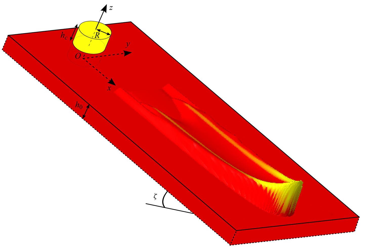
Figure 1. A plane with a layer of  $750\text {--}1000\ \mathrm {\mu }\textrm {m}$ spherical glass beads stuck to the surface is inclined at an angle
  $\zeta$ to the horizontal. The bed is coated with an erodible layer of
  $160\text {--}200\ \mathrm {\mu }\textrm {m}$ diameter red sand, of thickness
  $h_0$. A volume
  $V$ of yellow sand, with the same frictional properties, is then released on top of this layer from a hollow cylinder of radius
  $R=1.5\ \textrm {cm}$ filled to the required height
  $h_c$.
An avalanche is initiated by manually releasing a finite volume  $V = h_c{\rm \pi} R^2$ of yellow sand from a cylinder of radius
  $R=1.5\ \textrm {cm}$ filled to the required height
  $h_c$, approximately 80 cm from the end of the chute, on top of the red sand layer. The cylinder is lifted quickly and perpendicularly to the plane such that any non-normal releases are evident due to instantaneous symmetry breaking and are repeated, ensuring that the results are reproducible. The red and yellow sands are comprised of the same material with identical frictional properties, and differ only in colour. When the cylinder is raised, yellow particles spread from the downslope edge like a small inclined column collapse (Maeno et al. Reference Maeno, Hogg, Sparks and Matson2013), before forming an avalanche that travels downslope whilst eroding the red sand at the flow front and depositing particles behind. The point of release defines the origin of a coordinate system
  $Oxyz$ with the
  $x$-axis pointing downslope, the
  $y$-axis across the slope (with
  $y=0$ at the midpoint of the width of the plane) and the
  $z$-axis pointing normal to the rough plane at
  $z=0$. Evolution of the avalanche is captured in still images, which will be shown here in their raw formats aside from cropping, at a rate of 10 frames per second with a Canon 7D Mark II camera that is mounted perpendicularly to the inclined plane.
The behaviour of the avalanche that forms after the initial column collapse is dependent on the slope inclination angle, static layer thickness and volume of material initially released from the cylinder. While the values of these parameters, for which different types of behaviour can be observed, are dependent on the frictional properties of both the grains and the rough bed, the results are qualitatively reproducible on different experimental set-ups and using alternative materials. For example, Edwards et al. (Reference Edwards, Viroulet, Kokelaar and Gray2017) observed some similar avalanche behaviours to those presented here for flows of carborundum particles on a rough bed of spherical glass beads.
2.1. Decaying avalanche experiments
The release of a small volume  $V=5\ \textrm {ml}$ of yellow sand on an erodible layer of red sand of thickness
  $h_0 = h_{stop}(33.5^{\circ }) \approx 2.0\ \textrm {mm}$, inclined at the same
  $33.5^{\circ }$ angle at which the red sand was deposited, is shown in figure 2. The initial avalanche that forms shrinks in size (both width and height) before coming to rest 66 cm downslope. Much of the yellow sand is deposited in the first 20 cm of propagation and no yellow grains are clearly visible at all beyond 40 cm in the
  $x$-direction. The avalanche is therefore comprised entirely of red particles in the latter stages of movement, which implies that it must propagate downslope whilst undergoing a continuous exchange of particles between the mobile bulk flow and the erodible static layer ahead of it. Such decaying avalanches are observed over a range of slope angles, dependent on the volume of the release.

Figure 2. A sequence of overhead photos taken at 1.2 s time intervals (a–e) showing a 5 ml volume of  $160\text {--}200\ \mathrm {\mu }\textrm {m}$ diameter yellow sand released from a
  $R=1.5\ \textrm {cm}$ radius cylinder on top of an
  $h_0 = h_{stop}(33.5^{\circ }) \approx 2.0\ \textrm {mm}$ deep erodible layer of initially static red sand, on a rough plane inclined at
  $\zeta =33.5^{\circ }$. An avalanche, which is initially formed entirely of yellow sand, propagates to
  $x\approx 66\ \textrm {cm}$ downslope before coming to rest, undergoing an exchange of particles with the red sand substrate layer whilst doing so. The red and yellow sands are comprised of the same material with identical frictional properties and they only differ in colour. The bed is made rough by attaching a monolayer of
  $750\text {--}1000\ \mathrm {\mu }\textrm {m}$ diameter spherical glass beads. A movie showing the time-dependent evolution is available in the online supplementary material available at https://doi.org/10.1017/jfm.2021.34 and https://doi.org/10.17632/s8c6dws3s4.1.
2.2. Growing avalanche experiments
A qualitatively different avalanche over an identical  $2.0\ \textrm {mm}$ thick erodible layer is shown in figure 3. This differs from the previous experiment in that the inclination angle is raised to
  $34.0^{\circ }$ after preparation of the erodible layer at
  $33.5^{\circ }$, and a greater volume
  $V=10\ \textrm {ml}$ of yellow sand is released. Since the thickness of the deposit left by the slowest steady uniform flow at the
  $34.0^{\circ }$ experimental slope angle,
  $h_{stop}(34.0^{\circ })$, is now smaller than the erodible layer thickness,
  $h_0$, there is an abundance of erodible red sand ahead of the avalanche. This leads to a positive net erosion rate, so the avalanche continuously grows in size whilst digging out a widening trough as it propagates downslope. A consequence of this is that yellow particles from the cylinder are transported further than before. Much of the yellow sand release is deposited in the first 20 cm of travel, but the yellow-particle concentration then decays slowly, reaching zero by approximately 67 cm downslope. Such growing avalanches are only found here to occur when the erodible layer thickness is deeper than the value of
  $h_{stop}(\zeta )$ corresponding to the avalanche slope angle
  $\zeta$.
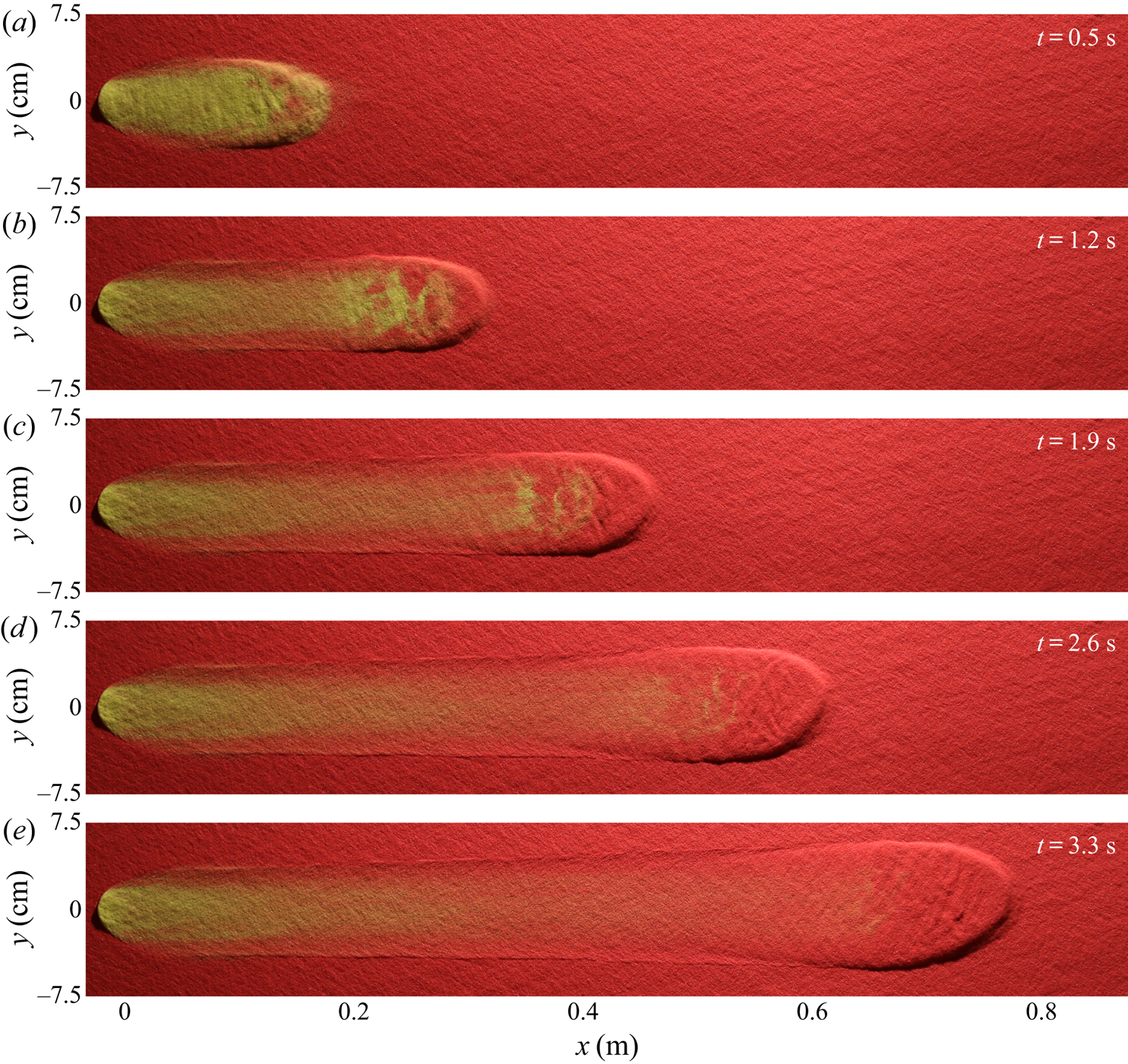
Figure 3. A sequence of overhead photos taken at 0.7 s time intervals (a–e) showing a 10 ml volume of  $160\text {--}200\ \mathrm {\mu }\textrm {m}$ diameter yellow sand released from a
  $R=1.5\ \textrm {cm}$ radius cylinder on top of an
  $h_0 = h_{stop}(33.5^{\circ }) \approx 2.0\ \textrm {mm}$ deep static erodible layer of the same sand, but coloured red, on a rough plane inclined at
  $\zeta =34.0^{\circ }$. An avalanche forms that continuously grows by eroding more red sand from the static layer than is deposited behind the bulk flow, whilst the yellow sand from which it is originally comprised is eventually all exchanged with the erodible substrate. A movie showing the time-dependent evolution is available in the online supplementary material.
2.3. Steady avalanche experiments
An avalanche of  $10\ \textrm {ml}$ of yellow sand at
  $\zeta =34.0^{\circ }$ over an erodible layer of
  $h_0 = h_{stop}(34.0^{\circ }) \approx 1.7\ \textrm {mm}$ deep red sand is shown in figure 4. The avalanche propagates at a constant speed whilst eroding material ahead of the bulk flow front and depositing grains behind in its wake, in a near exact balance. This results in the deposition of grains in a leveed channel of almost constant width, after an initial transient region of approximately 10 cm in length. These observations suggest that the avalanche reaches a steady state, which could travel indefinitely so long as the slope angle and deposit thickness remain constant. Although the avalanche itself propagates steadily, its composition becomes increasingly made up of red grains eroded from the static layer, whilst the number of visible yellow particles continuously decreases. Although there are still some yellow particles visible just behind the bulk head up to approximately 73 cm down the plane, the behaviour of the avalanche suggests that, if allowed to travel a short distance further, it will reach a steady state consisting entirely of red particles.
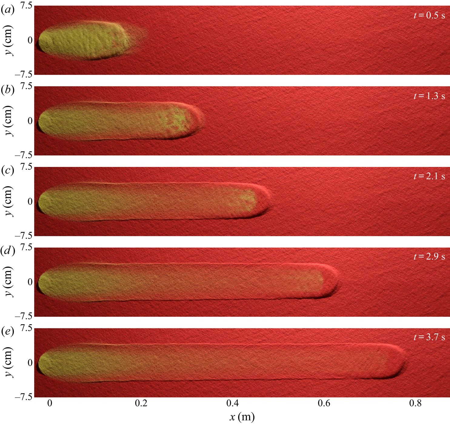
Figure 4. A sequence of overhead photos taken at 0.8 s time intervals (a–e) showing a 10 ml volume of  $160\text {--}200\ \mathrm {\mu }\textrm {m}$ diameter yellow sand released from a
  $R=1.5\ \textrm {cm}$ radius cylinder on top of an
  $h_0 = h_{stop}(34.0^{\circ }) \approx 1.7\ \textrm {mm}$ deep static erodible layer of the same sand, but coloured red, on a rough plane inclined at
  $\zeta =34.0^{\circ }$. An avalanche, which is initially formed entirely of yellow sand, propagates steadily downslope by undergoing a finely balanced exchange of particles with the red sand-substrate layer, such that all of the original yellow particles are eventually deposited whilst the avalanche itself maintains a constant speed and size. A movie showing the time-dependent evolution is available in the online supplementary material.
Different steady states are possible at, or near to, this slope angle for this particular granular system, according to experimental observations by Viroulet et al. (Reference Viroulet, Edwards, Kokelaar and Gray2019). Despite this, decreasing the slope angle just below a  $34.0^{\circ }$ inclination, for which a steady state was found above, results in a decaying avalanche. On the other hand, increasing the slope angle just above
  $34.0^{\circ }$ produces different steady states with slightly increasing leveed-channel widths. However, for sufficiently steep inclinations, more complicated avalanching behaviours also occur that do not result in steady states, and which will be investigated below.
2.4. Shedding material and secondary avalanches
An avalanche of  $10\ \textrm {ml}$ of yellow sand at
  $\zeta =35.5^{\circ }$ over an erodible layer of
  $h_0 = h_{stop}(35.5^{\circ }) = 1.0\ \textrm {mm}$ deep red sand is shown in figure 5. The initial collapse of material from the cylinder produces an avalanche that has a greater amplitude and greater leveed-channel width than the steady state for this slope angle. As a result, the avalanche deposits material soon after its formation as small chevron-shaped deposits at
  $x\approx 22\ \textrm {cm}$ and
  $x\approx 30\ \textrm {cm}$ downslope, in the middle of the channel (figure 5d,e). This shedding of material corresponds to a gradually decreasing channel width further downstream. Yellow particles released from the cylinder are transported further along the channel than in previous experiments, being visible in the shedding deposits, as well as still being present in the avalanche as it approaches the end of the plane, as in the steady state regime.
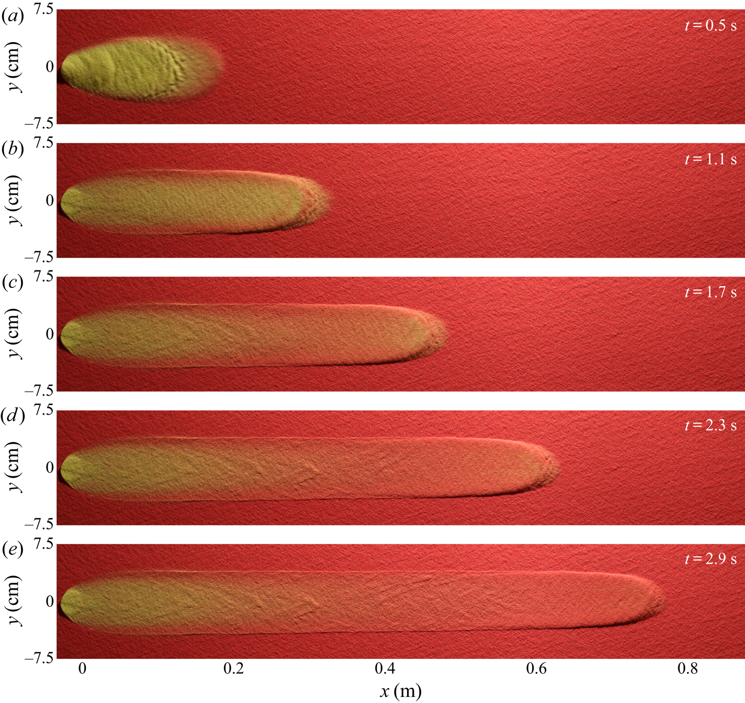
Figure 5. A sequence of overhead photos taken at 0.6 s time intervals (a–e) showing a 10 ml volume of  $160\text {--}200\ \mathrm {\mu }\textrm {m}$ diameter yellow sand released from a
  $R=1.5\ \textrm {cm}$ radius cylinder on top of an
  $h_0 = h_{stop}(35.5^{\circ }) \approx 1.0\ \textrm {mm}$ deep static erodible layer of the same sand, but coloured red, on a rough plane inclined at
  $\zeta =35.5^{\circ }$. The avalanche that forms from the release of yellow sand quickly sheds excess grains in chevron-shaped deposits, visible at
  $x\approx 22\ \textrm {cm}$ and
  $x\approx 30\ \textrm {cm}$ in panels (d,e), which causes the channel width to decrease whilst the bulk flow continues to propagate downslope, exchanging particles with the red sand-substrate layer as it does so. A movie showing the time-dependent evolution is available in the online supplementary material.
For the final experiment, the slope inclination of  $35.5^{\circ }$ and red sand depth
  $h_0 = h_{stop}(35.5^{\circ }) = 1.0\ \textrm {mm}$ depth remain as in the previous experiment, but the volume of yellow sand released from the cylinder is increased to 20 ml (figure 6). The shedding behaviour occurs more rapidly due to the larger volume of material released onto the erodible layer, and the chevron-shaped deposits close to the initial collapse have enough momentum themselves to propagate some distance further downslope as secondary avalanches (figure 6c–e), which transport yellow grains even further downslope.
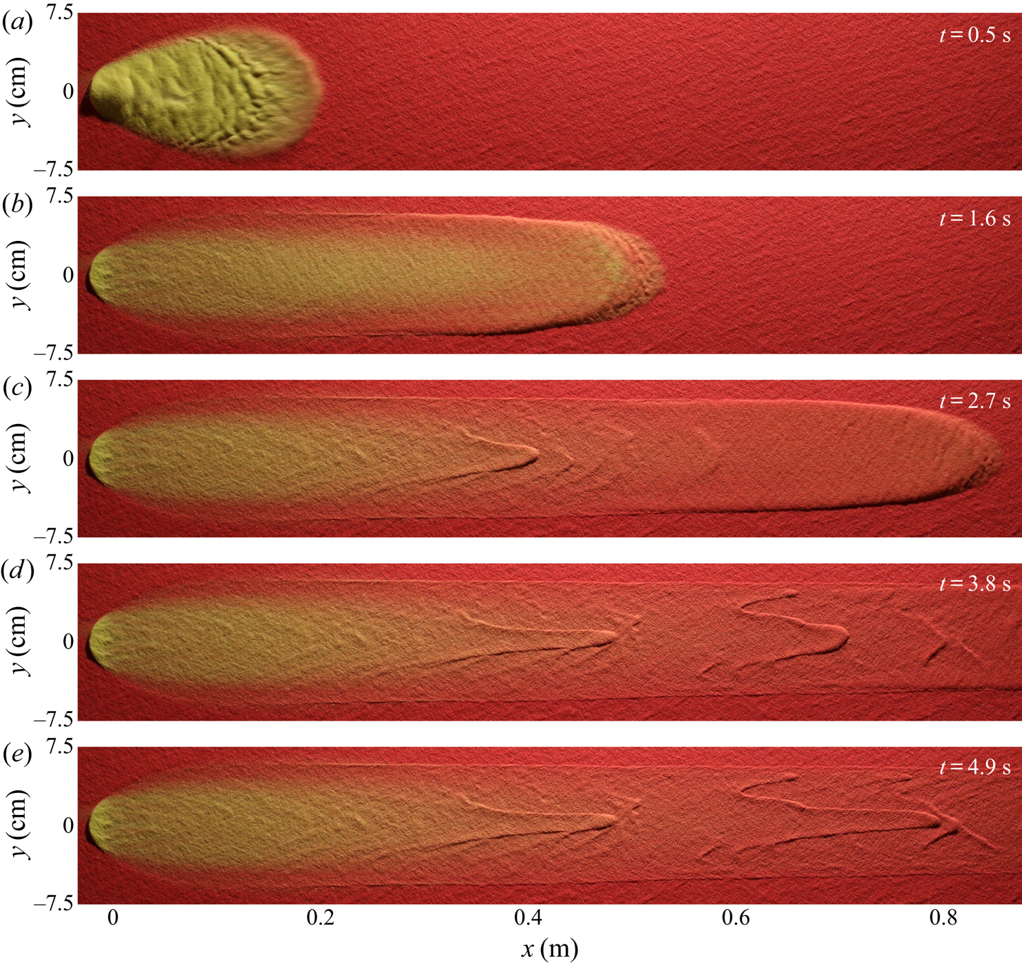
Figure 6. A sequence of overhead photos taken at 1.1 s time intervals (a–e) showing a 20 ml volume of  $160\text {--}200\ \mathrm {\mu }\textrm {m}$ diameter yellow sand released from a
  $R=1.5\ \textrm {cm}$ radius cylinder on top of an
  $h_0 = h_{stop}(35.5^{\circ }) \approx 1.0\ \textrm {mm}$ deep static erodible layer of the same sand, but coloured red, on a rough plane inclined at
  $\zeta =35.5^{\circ }$. The avalanche undergoes extreme shedding of excess yellow sand particles from which it is originally formed, such that the deposits have sufficient momentum to form secondary avalanches that can be seen to travel from
  $x\approx 40\ \textrm {cm}$ to
  $x\approx 48\ \textrm {cm}$ between panels (c,d) or from
  $x\approx 70\ \textrm {cm}$ to
  $x\approx 80\ \textrm {cm}$ between panels (d,e). A movie showing the time-dependent evolution is available in the online supplementary material.
3. Governing equations
The shallow granular flows described in § 2 are modelled using Edwards et al.'s (Reference Edwards, Viroulet, Kokelaar and Gray2017) avalanche equations (a two-dimensional generalization of the depth-averaged  $\mu (I)$-rheology of Gray & Edwards Reference Gray and Edwards2014), with a hysteretic basal friction rule for granular flows (Edwards et al. Reference Edwards, Russell, Johnson and Gray2019). The mixing of red and yellow grains is captured by Lagrangian tracking of the three-dimensional position of yellow grains from the initial release, and then inference of a depth-averaged concentration from their individual positions.
3.1. Depth-averaged equations with viscous dissipation
The shallow-water-like avalanche framework of Edwards et al. (Reference Edwards, Viroulet, Kokelaar and Gray2017) defines the thickness  $h$ and depth-averaged velocity
  $\boldsymbol {\bar {u}}=(\bar {u},\bar {v})$ through the entire layer, rather than explicitly resolving the interface between static and flowing layers in the normal direction to the chute or the erosion and deposition rates between them. Whilst this is a crude approximation, in that an avalanche is assumed to be either moving or static throughout its entire depth, it is a reasonable one for the shallow erodible layers studied here. The depth-averaged mass and momentum balance equations are therefore given by
 \begin{gather} \dfrac{\partial h}{\partial t} + \boldsymbol{\nabla} \boldsymbol{\cdot} \left(h \bar{\boldsymbol{u}}\right) = 0, \end{gather}
 \begin{gather} \dfrac{\partial}{\partial t}\left(h\boldsymbol{\bar{u}}\right) + \boldsymbol{\nabla} \boldsymbol{\cdot} \left(h \bar{\boldsymbol{u}} \otimes \bar{\boldsymbol{u}}\right) + \boldsymbol{\nabla}\left(\frac{1}{2} h^2 g\cos{\zeta}\right) = hg\boldsymbol{S} \cos{\zeta} + \boldsymbol{\nabla} \boldsymbol{\cdot} \left(\nu h^{3/2}\bar{\boldsymbol{D}}\right), \end{gather}
where g is the constant of gravitational acceleration,  $\nu$ is a coefficient in the depth-averaged kinematic granular viscosity
  $\nu h^{1/2}/2$, $\boldsymbol {\nabla } = (\partial /\partial x,\partial /\partial y)$ is the two-dimensional gradient operator, ‘
 $\cdot$’ is the dot product and
  $\otimes$ is the dyadic product. The non-dimensional net acceleration,
 \begin{equation} \boldsymbol{S} = \tan{\zeta}\boldsymbol{i} - \mu_b\boldsymbol{e}, \end{equation}
consists of the components of gravity and effective basal friction, where  $\mu _b$ is the basal friction coefficient (a function of flow thickness and Froude number
  $Fr=|\bar {\boldsymbol {u}}|/\sqrt {gh\cos \zeta }$),
  $\boldsymbol {i}$ is the downslope unit vector and the direction of the frictional force is determined by
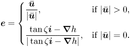 \begin{equation} \boldsymbol{e} = \begin{cases} \dfrac{\boldsymbol{\bar{u}}}{|\boldsymbol{\bar{u}}|}, & \text{if}\ |\boldsymbol{\bar{u}}|>0,\\ \dfrac{\tan\zeta\boldsymbol{i}-\boldsymbol{\nabla} h}{|\tan\zeta\boldsymbol{i}-\boldsymbol{\nabla} h|}, & \text{if}\ |{\bar{\boldsymbol{u}}}|=0. \end{cases} \end{equation}
The final, ‘viscous’, term on the right-hand side of (3.2) arises from the inclusion of in plane deviatoric stresses in the depth-averaged (Gray & Edwards Reference Gray and Edwards2014)  $\mu (I)$-rheology (GDR-MiDi 2004; Jop, Forterre & Pouliquen Reference Jop, Forterre and Pouliquen2006) with Pouliquen's (Reference Pouliquen1999a) dynamic friction rule. The depth-integrated strain-rate tensor
  $\bar {\boldsymbol {D}}$ is given by
 \begin{equation} \bar{\boldsymbol{D}} = \tfrac{1}{2}\left(\bar{\boldsymbol{L}} + \bar{\boldsymbol{L}}^{\mathrm{T}}\right), \end{equation}
where  $\bar {\boldsymbol {L}}=\boldsymbol {\nabla }\bar {\boldsymbol {u}}$ is the two-dimensional gradient of the depth-averaged velocity. The coefficient
 \begin{equation} \nu = \frac{2}{9} \frac{\mathscr{L}\sqrt{g}}{\beta} \frac{\sin{\zeta}}{\sqrt{\cos{\zeta}}} \left( \frac{\tan{\zeta_2} - \tan{\zeta}}{\tan{\zeta} - \tan{\zeta_1}} \right), \end{equation}
is explicitly determined by the depth-integration process. The parameters  $\mathscr {L}$,
  $\beta$,
  $\zeta _1$ and
  $\zeta _2$ follow from Pouliquen's (Reference Pouliquen1999a) dynamic basal friction rule, which is equivalent to the dynamic part of Edwards et al.'s (Reference Edwards, Russell, Johnson and Gray2019) friction rule used here. Values of the parameters taken in this paper are those measured by Viroulet et al. (Reference Viroulet, Edwards, Kokelaar and Gray2019) and Edwards et al. (Reference Edwards, Viroulet, Kokelaar and Gray2017), which are summarized in table 1. The corresponding values of
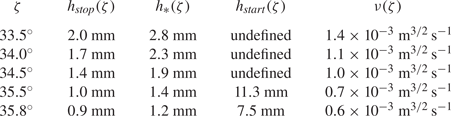
  $\nu (\zeta )$ are given in table 2, alongside critical flow thicknesses associated with the friction rule, for the various experimental and numerical slope angles.
Table 1. Material properties for flows of sand on a bed of glass beads, measured by Viroulet et al. (Reference Viroulet, Edwards, Kokelaar and Gray2019) and Edwards et al. (Reference Edwards, Viroulet, Kokelaar and Gray2017).
Table 2. Critical layer thicknesses and coefficients  $\nu (\zeta )$ in the depth-averaged viscosity
  $\nu h^{1/2}/2$ for various different slope angles, with the material properties for sand in table 1.
3.2. Non-monotonic friction coefficient for hysteresis and particle deposition
The expression used here for the basal friction coefficient  $\mu _b(h, Fr)$ is that of Edwards et al. (Reference Edwards, Russell, Johnson and Gray2019),
 $$\begin{align}{\mu_b(h,Fr)=} \tan \zeta_1 + \frac{\tan \zeta_2 - \tan \zeta_1}{1 + h \beta/\mathscr{L}(Fr+\Gamma)}, & \text{$Fr \geq \beta_*$}, \hskip2.6pc (3.7)\nonumber\\
\left(\dfrac{Fr}{\beta_*}\right)\left(\tan \zeta_1 + \frac{\tan \zeta_2 - \tan \zeta_1}{1 + h \beta/\mathscr{L}(\beta_*+\Gamma)} - \tan \zeta_3 \right.\nonumber \\
\left.\qquad\quad - \frac{\tan \zeta_2 - \tan \zeta_1}{1 + h /\mathscr{L}}\right) + \tan \zeta_3 + \frac{\tan \zeta_2 - \tan \zeta_1}{1 + h /\mathscr{L}}, & \text{$0 < Fr \leq \beta_*$}, \hskip1.1pc (3.8)\nonumber\\
\min\left( \tan \zeta_3 + \frac{\tan \zeta_2 - \tan \zeta_1}{1 + h/\mathscr{L}}, |\tan \zeta\boldsymbol{i}-\nabla h| \right), & \text{$Fr=0$}, \hskip2.99pc (3.9)\nonumber
\end{align}$$
$$\begin{align}{\mu_b(h,Fr)=} \tan \zeta_1 + \frac{\tan \zeta_2 - \tan \zeta_1}{1 + h \beta/\mathscr{L}(Fr+\Gamma)}, & \text{$Fr \geq \beta_*$}, \hskip2.6pc (3.7)\nonumber\\
\left(\dfrac{Fr}{\beta_*}\right)\left(\tan \zeta_1 + \frac{\tan \zeta_2 - \tan \zeta_1}{1 + h \beta/\mathscr{L}(\beta_*+\Gamma)} - \tan \zeta_3 \right.\nonumber \\
\left.\qquad\quad - \frac{\tan \zeta_2 - \tan \zeta_1}{1 + h /\mathscr{L}}\right) + \tan \zeta_3 + \frac{\tan \zeta_2 - \tan \zeta_1}{1 + h /\mathscr{L}}, & \text{$0 < Fr \leq \beta_*$}, \hskip1.1pc (3.8)\nonumber\\
\min\left( \tan \zeta_3 + \frac{\tan \zeta_2 - \tan \zeta_1}{1 + h/\mathscr{L}}, |\tan \zeta\boldsymbol{i}-\nabla h| \right), & \text{$Fr=0$}, \hskip2.99pc (3.9)\nonumber
\end{align}$$
where the constant non-dimensional parameters  $\beta$,
  $\zeta _1, \zeta _2, \zeta _3$ and length
  $\mathscr {L}$ are measured from independent experiments as best fits to the inverse functions of the slope angle-dependent critical layer thicknesses
  $h_{stop}(\zeta )$ and
  $h_{start}(\zeta )$. Since the form of these curves means that the non-dimensional constants are somewhat tuneable, it is perhaps more intuitive to consider the critical thicknesses
  $h_{stop}(\zeta )$ and
  $h_{start}(\zeta )$ themselves as the two important outputs that parameterize the friction rule. The remaining non-dimensional constants
  $\beta _*$ and
  $\varGamma$ are also determined independently of the avalanche experiments as a pair of best fits to the empirical steady uniform flow relationship between the ratio of the flow thickness
  $h$ to
  $h_{stop}(\zeta )$ and the Froude number.
This parameterization follows Pouliquen & Forterre (Reference Pouliquen and Forterre2002) in describing the experimentally observed hysteresis in granular avalanches through dynamic (3.7) to static (3.9) friction regimes via an intermediate regime (3.8) in which friction decreases with flow speed. The (3.7)–(3.9) extend the expressions given by Pouliquen & Forterre (Reference Pouliquen and Forterre2002) in three main ways: they describe non-spherical grains (Edwards et al. Reference Edwards, Viroulet, Kokelaar and Gray2017), they capture the difference between the thickness  $h_*$ of the slowest possible steady uniform flow and the smaller thickness
  $h_{stop}$ of the deposit that it leaves (Edwards et al. Reference Edwards, Viroulet, Kokelaar and Gray2017, Reference Edwards, Russell, Johnson and Gray2019) and they provide a quantitative description of the friction in the intermediate region using an experimentally inferred functional form (Russell et al. Reference Russell, Johnson, Edwards, Viroulet, Rocha and Gray2019). A derivation of this friction rule, and further details of how the parameters are measured experimentally, are given by Edwards et al. (Reference Edwards, Viroulet, Kokelaar and Gray2017, Reference Edwards, Russell, Johnson and Gray2019).
3.3. Particle tracking
In order to model the erosion, transport and deposition of grains by the avalanche, the three-dimensional trajectories of point particles are calculated. All of these particles are given initial positions within the confines of the experimental release cylinder and thus represent yellow grains, such that regions of three-dimensional space containing no tracked particles are assumed to be comprised entirely of red grains. A depth-averaged red-particle concentration  $\bar {\phi }$ can then be inferred by calculating the relative volume occupied by yellow particles in each grid cell, which allows the erosion-deposition process to be visualized as an exchange of coloured particles on the surface as in the experiments. Note that although this colour exchange has previously been modelled by Viroulet et al. (Reference Viroulet, Edwards, Kokelaar and Gray2019), they did this by using a large-particle-transport-like equation (Gray & Kokelaar Reference Gray and Kokelaar2010) that assumed the existence of an instantaneously and sharply segregated layer of yellow on top of red sand. This method only allowed for movement of grains relative to the bulk flow as a result of vertical shear rather than by tracking their three-dimensional positions, and resulted in unphysical shocks between regions of different colour for certain types of avalanche behaviour.
The motion of a particle at position  $\boldsymbol{x}_p =(x_p,y_p,z_p)$ that is advected by a divergence-free three-dimensional velocity field
  $(u,v,w)$, in which
 \begin{equation} \dfrac{\partial u}{\partial x} + \dfrac{\partial v}{\partial y} + \dfrac{\partial w}{\partial z} = 0, \end{equation}
with no flux through the base of the flow, i.e.  $w(z=0)=0$, is determined by
 \begin{equation} \dfrac{\mathrm{d} x_p}{\mathrm{d} t} = u(\boldsymbol{x}_p), \quad \dfrac{\mathrm{d} y_p}{\mathrm{d} t} = v(\boldsymbol{x}_p), \quad \dfrac{\mathrm{d} z_p}{\mathrm{d} t} = w(\boldsymbol{x}_p)={-}\int_0^{z_p}\left(\dfrac{\partial u}{\partial x} + \dfrac{\partial v}{\partial y}\right)\,\textrm{d}z. \end{equation}
Defining a non-dimensional vertical particle position, between the base  $z=0$ and the free surface
  $z=h(x,t)$, as
  $\varPhi _p = z_p / h(x,t)$ allows the dimensionless vertical motion to be written, by using (3.11c), as
 \begin{equation} \dfrac{\mathrm{d} \varPhi_p}{\mathrm{d} t} = \dfrac{1}{h}\dfrac{\mathrm{d} z_p}{\mathrm{d} t} - \dfrac{\varPhi_p}{h}\dfrac{\mathrm{d} h}{\mathrm{d} t} ={-}\dfrac{1}{h} \int_0^{z_p}\left(\dfrac{\partial u}{\partial x} + \dfrac{\partial v}{\partial y}\right)\,\textrm{d}z - \dfrac{\varPhi_p}{h}\dfrac{\mathrm{d} h}{\mathrm{d} t}. \end{equation}
Expressions for the non-depth-averaged downslope and cross-slope velocity components of the vector  $\boldsymbol {u}=(u,v)$ are required in order to calculate the movement of particles from the depth-averaged equations of motion. The components of the velocity vector parallel to the slope are assumed to take the following general form in terms of its depth-averaged counterpart,
 \begin{equation} \boldsymbol{u} = f(\varPhi)\boldsymbol{\bar{u}}, \end{equation}
for an arbitrary function  $f(\varPhi )$ and
  $\varPhi = z/h$. In this paper a linear variation with depth (e.g. Gray & Thornton Reference Gray and Thornton2005) will be assumed, i.e.
 \begin{equation} f(\varPhi) = \alpha + 2(1-\alpha)\varPhi, \end{equation}
for a parameter  $0 \leq \alpha \leq 1$. This allows the horizontal velocity profiles to vary from simple shear, for
  $\alpha =0$, to plug flow, for
  $\alpha =1$, and linear shear with basal slip for intermediate values. Baker et al. (Reference Baker, Barker and Gray2016) showed that a Bagnold velocity profile can be closely represented with a shear parameter value of
  $\alpha =1/7$, which will be used here. In general,
 \begin{equation} \dfrac{\partial u}{\partial x} + \dfrac{\partial v}{\partial y} = \left(\dfrac{\partial \bar{u}}{\partial x} + \dfrac{\partial \bar{v}}{\partial y} \right)f(\varPhi) - \left(\bar{u}\dfrac{\partial h}{\partial x} + \bar{v}\dfrac{\partial h}{\partial y} \right) \dfrac{\varPhi f^{\prime}(\varPhi)}{h}, \end{equation}
where  $f^{\prime }(\varPhi )$ is the derivative of
  $f(\varPhi )$. The dimensionless vertical particle motion can then be determined, by substituting (3.15) into (3.12) and evaluating the integral in terms of
  $\varPhi$, to give
 \begin{equation} \dfrac{\mathrm{d} \varPhi_p}{\mathrm{d} t} ={-}\dfrac{1}{h} \left[h \left(\dfrac{\partial \bar{u}}{\partial x} + \dfrac{\partial \bar{v}}{\partial y} \right)F(\varPhi_p) + \left(\bar{u}\dfrac{\partial h}{\partial x} + \bar{v}\dfrac{\partial h}{\partial y} \right)(F(\varPhi_p) - \varPhi_pf(\varPhi_p))\right] - \dfrac{\varPhi_p}{h}\dfrac{\mathrm{d} h}{\mathrm{d} t}, \end{equation}
where  $F(\varPhi _p) = \int _0^{\varPhi _p} f(\varPhi ) d\varPhi$ is the integral of the velocity profile function
  $f(\varPhi )$ with respect to
  $\varPhi$. This can be simplified by expanding the total derivative
  $\mathrm {d}h/\mathrm {d}t$, substituting for the velocity components from (3.13) and then cancelling common terms using conservation of mass (3.1), to give the general functional form of the dimensionless vertical motion of particles as
 \begin{equation} \dfrac{\mathrm{d} \varPhi_p}{\mathrm{d} t} = \dfrac{1}{h}\dfrac{\partial h}{\partial t}(F(\varPhi_p)-\varPhi_p). \end{equation}
The three-dimensional particle motion is therefore completely determined by (3.11a,b) and (3.17), which can be calculated at the same time as solving the depth-averaged governing equation (3.1)–(3.2) numerically.
A semi-discrete non-oscillatory shock-capturing scheme (Kurganov & Tadmor Reference Kurganov and Tadmor2000) is used to time integrate the governing equations (3.1)–(3.2). Details of the method, as applied to granular flows with depth-averaged viscosity, are given in Edwards et al. (Reference Edwards, Russell, Johnson and Gray2019). The particle transport equations (3.11a,b) and (3.17) for each particle are time integrated alongside the discretized conservation laws (3.1)–(3.2).
4. Numerical simulation of decaying, growing and steady avalanches
The depth-averaged mass and momentum balance equations (3.1)–(3.2) in conservative form, with the hysteretic friction rule for angular particles (3.7)–(3.9), are solved numerically in a configuration that replicates the experiments of § 2. The computational domain is  $-5\ \textrm {cm} \leq x \leq 95\ \textrm {cm}$ and
  $-7.5\ \textrm {cm} \leq y \leq 7.5\ \textrm {cm}$, discretized to
  $1000\times 150$ finite volume cells (1 grid point per mm). The initial conditions at
  $t=0$ are
  $h\bar {u}=h\bar {v}=0$ (initially static material),
  $h=h_c$ for
  $x^2+y^2 < R^2$ (representing the initial cylinder of grains) and
  $h=h_0$ elsewhere. As in experiments,
  $R=1.5\ \textrm {cm}$ and
  $h_c=V/({\rm \pi} R^2)$, where the volume
  $V$ is set to 5 ml, 10 ml or 20 ml. The flow reaches only the downstream boundary
  $x=x_d=95\ \textrm {cm}$, at which an outflow condition is imposed by linear extrapolation of the values of
  $h$ and
  $h\bar {u}$ from the final two columns of interior cells.
Three-dimensional particle tracking is initiated at time  $t=0$ by randomly distributing
  $N_p = 1.5$ million particles within the initial region of yellow grains,
  $x^2+y^2 < R^2$ and
  $h_0 \leq z \leq h_0 + h_c$, of the volume
  $V$. A depth-averaged red-particle concentration
  $\bar {\phi }$ can then be inferred from the locations of individual yellow particles by first rounding their horizontal positions to the nearest grid cell. In a grid cell of size
  $\delta x \times \delta y \times h$ with
  $n_p$ such particles, the depth-averaged red-particle concentration is then
 \begin{equation} \bar{\phi}_0 = 1 - \frac{n_p V}{N_p \delta x \delta y h}. \end{equation}
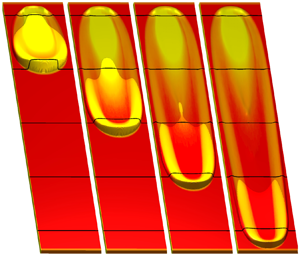
When the simulations commence, the cylinder collapses to form an avalanche that mobilizes initially static material ahead of the flow front as it propagates downslope. The behaviour of the avalanche depends upon the slope angle, the stationary layer thickness and the volume in the cylinder, as previously found by Edwards et al. (Reference Edwards, Viroulet, Kokelaar and Gray2017) and in the experiments performed here in § 2. Each experimental configuration will now be replicated in the numerics and the results will be shown as three-dimensional surface plots of the flow thickness  $h$ at three successive time intervals, viewed from an oblique angle. An artificial light source at the downslope end of the domain creates a shading effect that allows for variations in the flow thickness to be visualized, in the same way that the real lighting does in the experiments. The surface is coloured according to the depth-averaged red-particle concentration
  $\bar {\phi }$, such that regions where
  $\bar {\phi }=1$ (purely red-particle phases) appear red and regions where
  $\bar {\phi } \leq 0.6$ (where there are both red and yellow particles present through the flow depth at a given point) appear yellow. The colouring is biased towards highlighting surface particles (effectively as it is for an observer of the analogous experiments) so that it is not required to have
  $\bar {\phi }=0$ (purely yellow-particle phase) in order for the surface to appear yellow in colour. At the final simulated time, the flow thickness profile
  $h$ is plotted (and filled solid red) in both the downslope
  $x$-direction at the midpoint
  $y=0$ of the plane and in the cross-slope
  $y$-direction at locations
  $x=0.2\ \textrm {m}$,
  $x=0.4\ \textrm {m}$ and
  $x=0.6\ \textrm {m}$. All of the tracked particles whose interpolated positions lie in these two-dimensional planes will also be plotted on the cross-slope profiles as solid yellow markers.
4.1. Decaying avalanches
Simulations are first performed to model the colour change in the decaying avalanche shown in figure 2. The slope angle is set to  $\zeta =33.5^{\circ }$ and an initial layer thickness of
  $h_0 = 2.0\ \textrm {mm}$ is prescribed, which is equivalent to
  $h_{stop}(33.5^{\circ })=2.0\ \textrm {mm}$ at this inclination. The results are plotted as three-dimensional flow thickness surfaces coloured by red-particle concentration at 1.2 s time intervals in figure 7(a–c) and as cross-slope profiles at the latter time
  $t=2.9\ \textrm {s}$ in figure 7(d–f). On this shallow slope angle, the avalanche deposits material on top of the static layer and by
  $t=2.9\ \textrm {s}$ (figure 7c) has completely come to rest, with the front reaching
  $x \approx 0.5\ \textrm {m}$ downslope. A consequence of this net deposition of material and decrease in momentum of the avalanche is that the yellow particles from the cylinder are transported only a short distance downslope. In particular, the cross-slope profiles show that yellow particles are being deposited at
  $x=0.2\ \textrm {m}$ (figure 7d) and that the flow is composed entirely of red particles by
  $x=0.4\ \textrm {m}$ (figure 7e). Furthermore, the downslope profile in figure 12(a) shows that all of the yellow particles from the initial release are deposited behind the point at which the avalanche peak comes to rest.
Figure 7. Numerical simulation of a 5 ml release on a static layer of thickness  $h_0=h_{stop}(33.5^{\circ })=2.0\ \textrm {mm}$ and a slope angle of
  $\zeta =33.5^{\circ }$. The avalanche that forms from an initial cylindrical release comes to rest after propagating to
  $x \approx 0.5\ \textrm {m}$ downslope and no yellow particles are visible further than
  $x \approx 0.3\ \textrm {m}$ downslope. Oblique surface plots of the plane, plotted at times (a) 0.5 s, (b) 1.7 s and (c) 2.9 s, are coloured by the depth-averaged red-particle concentration
  $\bar {\phi }$ and an artificial light source at the downslope end provides visualization of the three-dimensional flow thickness, as in the experiments. Mobile regions of flow with non-zero momentum appear brighter due to an increased reflectance. Flow thickness
  $h$ (solid black lines and red filled area) and individual particle positions (yellow markers) are plotted in the cross-slope
  $y$-direction at (d)
  $x=0.2\ \textrm {m}$, (e)
  $x=0.4\ \textrm {m}$ and (f)
  $x=0.6\ \textrm {m}$ downslope for the final shown time
  $t=2.9\ \textrm {s}$. A movie showing the time-dependent evolution is available in the online supplementary material.
The downslope position of the avalanche wavefront  $x_w$ and the leveed-channel width
  $W$ (measured as the cross-slope distance between levee peaks) are compared to the experimental results in figure 13. This shows that the numerical avalanche reaches a shorter distance than the
  $0.66\ \textrm {m}$ travelled by the experimental one, despite the former propagating around
  $50\,\%$ faster than the latter before they come to rest. Furthermore, the leveed channel from the decaying avalanche simulation is approximately
  $25\,\%$ wider than that observed experimentally. This same behaviour was identified by Edwards et al. (Reference Edwards, Viroulet, Kokelaar and Gray2017), who postulated that it could be a consequence of needing to either modify the friction rule, resolve the interface between flowing and stationary regions in the vertical direction, or better capture the initial column collapse. The first of these ideas has been investigated in this paper without overcoming the problem of width discrepancy, and so it remains an open problem that might be solved with application of the alternative suggestions.
4.2. Growing avalanches
Next, the slope inclination is set to  $34.0^{\circ }$ and the static layer thickness to
  $h_0 = 1.7\ \textrm {mm}$, which is equivalent to
  $h_{stop}(33.5^{\circ })=1.7\ \textrm {mm}$ of the shallower
  $33.5^{\circ }$ angle and is greater than
 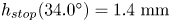 $h_{stop}(34.0^{\circ })=1.4\ \textrm {mm}$ of the current slope angle. This thick erodible layer provides an abundance of material for the avalanche to erode as it propagates downslope, which it does at a greater rate than it deposits. This results in a bulk flow that grows in size, as shown by coloured flow thickness surfaces at 1.3 s intervals in figure 8(a–c), whilst eroding a widening leveed trough, whose cross-slope profiles are plotted in figure 8(d–f). Despite the avalanche growing in size, there is still deposition of a large proportion of the yellow particles shortly after the initial column collapse, while a small number of yellow grains are transported with the avalanche front as it approaches the end of the domain. A U-shaped curve of yellow particles around the bulk avalanche head deposits grains inside and parallel to the leveed-channel walls with a lower red-particle concentration than at the midpoint
  $y=0$ of the plane. This curve is thinning as the avalanche propagates downslope, entraining an increasing number of red particles from the substrate layer as its width increases. An ever-decreasing amount of yellow grains is left in the trough that is eroded in the wake of the flow, as shown in figure 8(d–f), meaning that the avalanche is continuously exchanging particles with the stationary layer. The downslope profile in figure 12(b) shows that a yellow-particle layer of decreasing thickness below the free surface is deposited as the avalanche propagates, whilst there is still a yellow particle-rich head including a small region that have been overturned by recirculating red grains. The comparison of avalanche front position with time and leveed-channel width versus downslope location between simulations and experiments in figure 13 shows that the numerical growing avalanche propagates at a speed of
  $0.26\ \textrm {m}\,\textrm {s}^{-1}$, which is roughly
  $18\,\%$ faster than the experimental value of
  $0.22\ \textrm {m}\,\textrm {s}^{-1}$. It is also shown that the width of the leveed channel in the simulation grows from 10.1 cm at
  $x=0.2\ \textrm {m}$ downslope to 13.1 cm at
  $x=0.8\ \textrm {m}$ compared to a growth of 7.6 cm to 11.4 cm in the equivalent experiment, which represents a greater numerical width by a factor of
  $33\,\%$ initially and
  $15\,\%$ at the final recorded position.
Figure 8. Numerical simulation of a 10 ml release on a static layer of thickness  $h_0=h_{stop}(33.5^{\circ })=2.0\ \textrm {mm}$ and a slope angle of
  $\zeta =34.0^{\circ }$. The resulting avalanche continually grows in size as it propagates downslope, by eroding more particles from the stationary layer than are deposited in the lateral levees, whilst digging out a widening trough in its wake. This leads to more and more red grains being entrained by the avalanche and a reduction in the number of yellow particles with increasing downslope distance. Oblique surface plots of the plane coloured by the depth-averaged red-particle concentration
  $\bar {\phi }$ are plotted at times (a) 0.5 s, (b) 1.8 s and (c) 3.1 s. Flow thickness
  $h$ (solid black lines and red filled area) and individual particle positions (yellow markers) are plotted in the cross-slope
  $y$-direction at (d)
  $x=0.2\ \textrm {m}$, (e)
  $x=0.4\ \textrm {m}$ and (f)
  $x=0.6\ \textrm {m}$ downslope for the final shown time
  $t=3.1\ \textrm {s}$. A movie showing the time-dependent evolution is available in the online supplementary material.
4.3. Steady avalanches
The slope of the plane is kept at the same  $\zeta =34.0^{\circ }$ angle but the initial stationary layer thickness is now set to a thinner value of
  $h_0=1.4\ \textrm {mm}$, which is equivalent to
  $h_{stop}(34.0^{\circ })=1.4\ \textrm {mm}$ at this inclination. These conditions result in an avalanche that appears to propagate steadily downslope with an almost exact balance between net erosion and deposition of particles. The size and propagation speed of the bulk flow front are shown to be constant in figure 9(a–c), via coloured flow thickness surfaces plotted at 1.3 s intervals. Furthermore, cross-slope profiles in figure 9(d–f) show that the width of the channel between lateral levees, where material is deposited above the static layer thickness, remains virtually constant as the avalanche travels down the plane. Again there is the formation of a U-shaped yellow particles curve around the avalanche head, though the bands are thicker than those in the growing avalanche and as a result all of the yellow grains appear to have left the flow front by the final shown time (figure 9c). It also clearly evident from figure 9 that there is again a continually decreasing number of yellow particles being deposited by the avalanche as it propagates downslope, and that the mean red-particle concentration is lower than that of the growing avalanche at corresponding times, meaning that the rate of particle exchange between a steady avalanche and the static layer ahead of it is faster in comparison. In fact, the downslope profile in figure 12(c) explicitly demonstrates that the steady avalanche head contains fewer yellow particles than that of the growing type (figure 12b). The comparison of front position between simulations and experiments in figure 13(a) shows that the steady avalanche propagates at a near constant speed of
  $0.23\ \textrm {m}\,\textrm {s}^{-1}$, which is approximately
  $21\,\%$ faster than the experimental value of
  $0.19\ \textrm {m}\,\textrm {s}^{-1}$. The leveed channels are compared in figure 13(b), which shows that the width for the steady avalanche simulation remains close to 9.5 cm, compared to an almost constant experimental value of
  $7.4\ \textrm {cm}$. This is equivalent to an approximate
  $28\,\%$ over-prediction of width by the theory.

Figure 9. Numerical simulation of a 10 ml release on a static layer of thickness  $h_0=h_{stop}(34.0^{\circ })=1.7\ \textrm {mm}$ and a slope angle of
  $\zeta =34.0^{\circ }$. An avalanche forms that propagates in an apparently steady manner, maintaining a constant size and speed as it travels downslope due to the amount of grains eroded from the stationary layer being in a delicate balance with those deposited in the lateral levees. Oblique surface plots of the plane coloured by the depth-averaged red-particle concentration
  $\bar {\phi }$ are plotted at times (a) 0.5 s, (b) 1.8 s and (c) 3.1 s. Flow thickness
  $h$ (solid black lines and red filled area) and individual particle positions (yellow markers) are plotted in the cross-slope
  $y$-direction at (d)
  $x=0.2\ \textrm {m}$, (e)
  $x=0.4\ \textrm {m}$ and (f)
  $x=0.6\ \textrm {m}$ downslope for the final shown time
  $t=3.1\ \textrm {s}$. A movie showing the time-dependent evolution is available in the online supplementary material.
4.4. Numerical simulation of shedding and secondary avalanches
Numerical simulations are now performed with the slope angle increased to  $\zeta =35.8^{\circ }$ and the stationary layer is given a thickness of
  $h_0 = 0.9\ \textrm {mm}$, equivalent to
  $h_{stop}(35.8^{\circ })$ at the same inclination. At this steep slope angle and correspondingly thin layer ahead of the avalanche, it is forced to shed material in the centre of the channel between the lateral levees. As a result, whilst the three-dimensional surfaces, which are plotted at 1.4 s time intervals in figure 10(a–c), resemble those of a steady avalanche, there is in fact a net deposition of material. This is also apparent from the cross-slope profiles in figure 10(d–f) that show the depth of the channel between the levees is slightly greater than that of the initial layer, meaning that the avalanche has deposited some of its mass here. Interestingly, it is this particular avalanche behaviour that transports the yellow particles from the initial column the furthest of all. The bulk flow consists of a yellow-particle-rich U-shaped curve around the avalanche head for the entire distance that it propagates on this domain (figure 10c), whilst in this case the lateral bands of lower red particle concentration encompass the levees themselves as well as the inner lining of the channel walls. This is in contrast to all of the other types of avalanche studied here, which had exchanged most of their yellow grains with red particles from the static layer before they came to rest or reached the end of the plane. There is also a visibly thicker layer of yellow particles remaining in the deposit at
  $x=0.6\ \textrm {m}$ (figure 10f) than in any of the previous simulations in § 4, whilst the downslope profile plotted in figure 12(d) shows that the avalanche head contains more yellow grains than those too. This suggests that either shedding avalanches do indeed exhibit a slower exchange of particles with the erodible layer than all of the other behaviour types, or that an
  $\alpha =1/7$ shear rate in the downslope velocity profile (3.14) is not such a good approximation in this case. Furthermore, the cross-slope profiles show that the width between the lateral levees is decreasing with increasing downslope distance, which implies that the avalanche is either readjusting to a thinner and less massive steady state, or that it will continuously decay on a sufficiently long domain. This will be investigated later by performing numerical simulations in a frame of reference that moves with the avalanche.
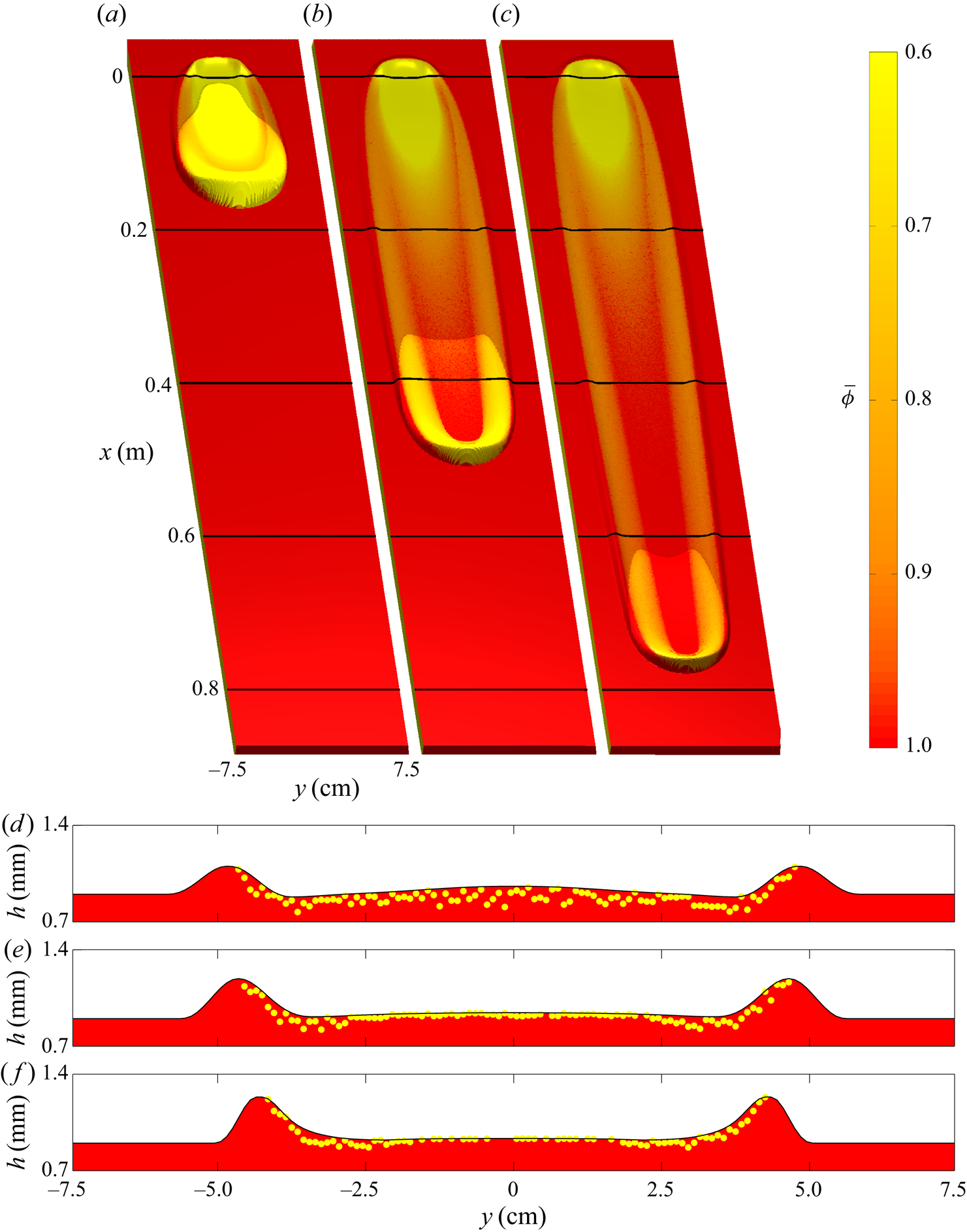
Figure 10. Numerical simulation of a 10 ml release on a static layer of thickness 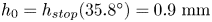 $h_0=h_{stop}(35.8^{\circ })=0.9\ \textrm {mm}$ and a slope angle of
  $\zeta =35.8^{\circ }$. Shortly after its formation the avalanche sheds a small amount of material in the centre of the leveed channel, whose width subsequently decreases slightly. The channel thickness is the same depth as the erodible layer, hence additional mass is continually deposited in the lateral levees. Oblique surface plots of the plane coloured by the depth-averaged red-particle concentration
  $\bar {\phi }$ are plotted at times (a) 0.5 s, (b) 1.9 s and (c) 3.3 s. Flow thickness
  $h$ (solid black lines and red filled area) and individual particle positions (yellow markers) are plotted in the cross-slope
  $y$-direction at (d)
  $x=0.2\ \textrm {m}$, (e)
  $x=0.4\ \textrm {m}$ and (f)
  $x=0.6\ \textrm {m}$ downslope for the final shown time
  $t=3.3\ \textrm {s}$. A movie showing the time-dependent evolution is available in the online supplementary material.
The avalanche front position and the leveed-channel width  $W$ are compared to experiments in figure 13, where it is shown that the numerical shedding avalanche propagates at around
  $14\,\%$ slower than the experimental equivalent. However, the leveed channel in the simulations is still wider than that of the experiments by 9.8 cm compared to 8.2 cm, or a factor of
  $20\,\%$, at
  $x=0.2\ \textrm {m}$ downslope and by 7.9 cm compared to 6.3 cm, or a factor of
  $25\,\%$, which is also the mean value for all recorded positions, at
  $x=0.8\ \textrm {m}$.
Next, the volume of material released from the cylinder is increased to  $V=20\ \textrm {ml}$ whilst the slope angle and stationary layer thickness are unchanged. In this case, there is an even greater excess of mass that the avalanche sheds quickly after the initial release from the cylinder. This leads to the formation of two secondary avalanches between the lateral levees that propagate a short distance before leaving chevron-shaped deposits, as shown by the surfaces plotted at 1.3 s intervals in figure 11(a–c). The results agree qualitatively with those of the experiment in figure 6, where there are two chevron-shaped deposits left by secondary avalanches. The numerical results also clearly show that the first chevron consists mainly of yellow particles and the second mainly of red, for which there is also some evidence of in the experiments. Cross-slope profiles of the final deposit, plotted in figure 11(d–f), show that the two successive chevron-shaped deposits leave thicker regions near the centre of the channel. The downslope profile in figure 12(e) shows that a greater number of yellow particles than any previous avalanche behaviours are both deposited in the channel and continue to propagate in the bulk head, although more yellow grains were released in this case. The cross-slope flow profiles also show that the leveed-channel depth is thicker than the stationary layer and that the width is again decreasing with increasing propagation distance, which implies that the avalanche is continuously losing mass as it travels downslope. Once again, this suggests that the avalanche is either continually decaying or readjusting to a smaller steady state regime. The long distance propagation behaviour of both the 10 ml and 20 ml volume shedding and secondary avalanche behaviours will be investigated in § 5.3 to determine which is the case for both.
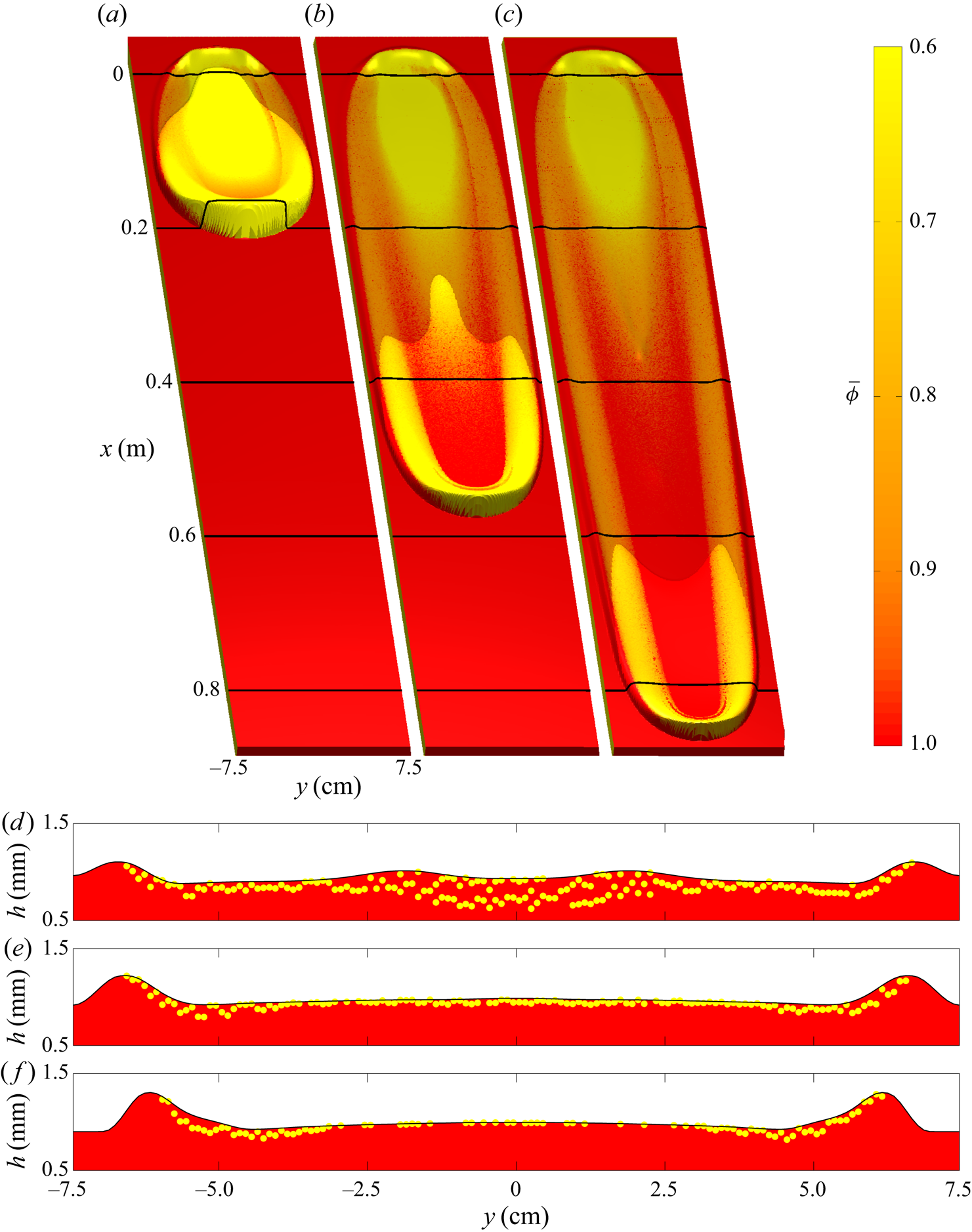
Figure 11. Numerical simulation of a 20 ml release on a static layer of thickness  $h_0=h_{stop}(35.8^{\circ })=0.9\ \textrm {mm}$ and a slope angle of
  $\zeta =35.8^{\circ }$. The avalanche sheds two chevron-shaped deposits at
  $x \approx 0.3\ \textrm {m}$ and
  $x \approx 0.5\ \textrm {m}$ downslope in the centre of the leveed channel, which then undergoes a reduction in width corresponding to the net loss of mass. Oblique surface plots of the plane coloured by the depth-averaged red-particle concentration
  $\bar {\phi }$ are plotted at times (a) 0.5 s, (b) 1.8 s and (c) 3.1 s. Flow thickness
  $h$ (solid black lines and red filled area) and individual particle positions (yellow markers) are plotted in the cross-slope
  $y$-direction at (d)
  $x=0.2\ \textrm {m}$, (e)
  $x=0.4\ \textrm {m}$ and (f)
  $x=0.6\ \textrm {m}$ downslope for the final shown time
  $t=3.1\ \textrm {s}$. A movie showing the time-dependent evolution is available in the online supplementary material.
Figure 12. Numerical simulations of (a) decaying, (b) growing, (c) steady flows, (d) shedding and (e) shedding with secondary avalanches. Downslope flow thickness profiles (solid black lines with solid red fill) and individual particle positions (yellow markers) are plotted in the downslope  $x$-direction at the cross-slope centre
  $y=0$ of the plane and at their final simulation times, which are shown in figures 7(c), 8(c), 9(c), 10(c) and 11(c) respectively. Movies showing the time-dependent evolution are available in the online supplementary material.
The comparison of avalanche front position with time and leveed-channel width versus downslope location between simulations and experiments in figure 13 shows that the shedding with secondary avalanche wavefront propagates at  $0.23\ \textrm {m}\,\textrm {s}^{-1}$, which is approximately
  $26\,\%$ slower than the experimental value of
  $0.29\ \textrm {m}\,\textrm {s}^{-1}$. It is also shown that the width of the leveed channel in the simulation decreases from 13.6 cm at
  $x=0.2\ \textrm {m}$ downslope to 11.4 cm at
  $x=0.8\ \textrm {m}$ compared to a reduction of 11.3 cm to 9.6 cm in the equivalent experiment, while the numerical estimation of width remains near the mean value of
  $21\,\%$ across all recorded locations.

Figure 13. A comparison of (a) downslope avalanche front position in time and (b) leveed-channel width against downslope location between experiments (markers) and simulations (solid lines) for each of the decaying (red), growing (green), steady (blue), shedding (black) and shedding with secondary avalanche (magenta) behaviours.
A phase diagram of the different avalanche behaviour types depending on the slope inclination angle and initial volume release is shown in figure 14. It is clear that for the release of a fixed volume, in particular  $V=20\ \textrm {ml}$, increasing
  $\zeta$ can change the resultant avalanche behaviour from decaying to steady, through to shedding and finally secondary avalanches. Alternatively, increasing the volume released on a fixed inclination increases the propensity for flow, e.g. changing a decaying avalanche to steady for
  $33.5^{\circ } \leq \zeta \leq 34.0^{\circ }$ or from steady to shedding and secondary avalanches for
  $\zeta = 35.5^{\circ }$. Note that growing avalanches do not appear on the phase diagram, since they require an abundantly thick stationary layer that is prepared on a shallower slope angle than that at which the material is released. There is good quantitative agreement between experiments and numerics about the type of behaviour that is observed according to inclination and volume, although shedding occurs for slightly shallower inclinations or smaller volumes in the former than the latter.
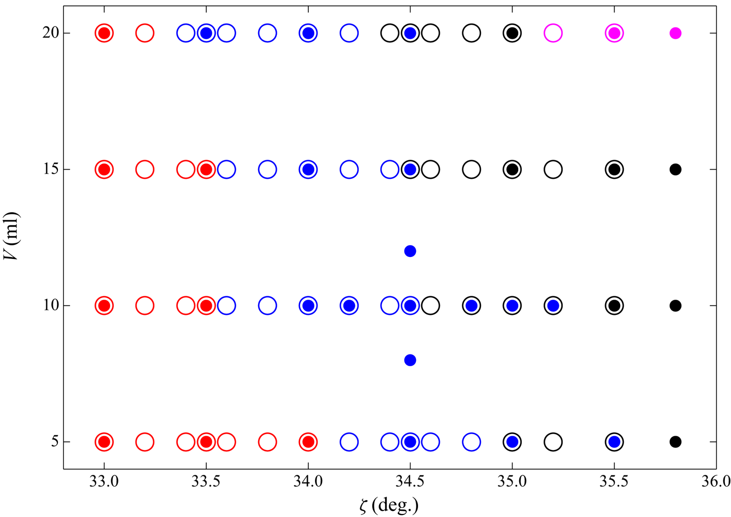
Figure 14. Phase diagram showing the inclination angles and initial volume release for which the various decaying (red), steady (blue), shedding (black) and shedding with secondary avalanche (magenta) behaviours are observed in experiments (hollow markers) and simulations (solid markers).
Note that the  $\zeta =35.8^{\circ }$ numerical slope angle is slightly steeper than the
  $35.5^{\circ }$ inclination on which the experimental shedding avalanche results of § 2.4 were obtained, and the corresponding stationary layer depth of
  $h_0 = h_{stop}(35.8^{\circ }) = 0.9\ \textrm {mm}$ is also slightly thinner than the experimental
 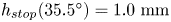 $h_{stop}(35.5^{\circ }) = 1.0\ \textrm {mm}$ deep layer. However, both the shedding and secondary avalanches do occur in simulations for these parameters replicating the experiments, though the behaviours are much less pronounced and so are harder to visualize than those of the numerical results presented here.
5. Long distance propagation behaviour in a travelling frame
Limits on both the physical size of an experimental plane and the computational demand of a numerical domain mean that, aside from the decaying case, the long distance propagation behaviour of the different types of avalanche are all unknown. Their behaviour can, however, be investigated numerically by transforming the governing equations into a travelling frame in a domain that contains all the flowing material. This allows efficient computation of avalanches that travel long distances relative to their own length.
5.1. Travelling frame equations
For a constant speed of the travelling frame  $u_f$ that takes different values, applying the change of coordinates
 \begin{equation} \tau=t-t_0,\quad \xi = x - u_f t,\quad\upsilon=y, \end{equation}
to the mass and momentum conservation laws (3.1)–(3.2) leads to a set of new governing equations in this frame, which are given in Edwards et al. (Reference Edwards, Viroulet, Kokelaar and Gray2017). The velocities of particles in the moving frame are obtained by making the coordinate transformation (5.1a–c) and following the derivation process in § 3.3, leading to particle transport equations,
 \begin{equation} \dfrac{\mathrm{d} \xi_p}{\mathrm{d} \tau} = u - u_f, \quad \dfrac{\mathrm{d} \upsilon_p}{\mathrm{d} \tau} = v, \quad \dfrac{\mathrm{d} \varPhi_p}{\mathrm{d} \tau} = \dfrac{1}{h}\left(\dfrac{\partial h}{\partial \tau}-u_f \dfrac{\partial h}{\partial \xi}\right)(F(\varPhi_p)-\varPhi_p). \end{equation}
As before, the discretized conservation law and particle positions in the moving frame are time integrated numerically. The boundary condition at the downslope end,  $\xi = 95\ \textrm {cm}$ is now an inflow, and a stationary layer of red particles is supplied by imposing
  $h=h_0$ and
  $h\bar {u}=0$ there. An outflow is imposed as in the lab frame, but now at the upstream boundary
  $\xi =-5\ \textrm {cm}$. The initial conditions of the travelling frame computations are taken from the laboratory frame numerical computations at a time
  $t=t_0$, when the avalanches have developed but have almost flowed out of the domain.
5.2. Long distance propagation of growing avalanches
The late-time behaviour of the growing avalanche of figure 8 (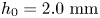 $h_0=2.0\ \textrm {mm}$,
  $\zeta =34^{\circ }$,
  $V=10\ \textrm {ml}$) is shown in figure 15. The avalanche continues to grow in length, width and height during the first 30 s of propagation, leaving gradually diverging lateral levees. The wake of the bulk flow front begins to break into a double-tail structure after 15 s (figure 15a), which extends in length during the next 30 s of propagation (figure 15b,c), but reaches a large steady state (figure 15c,d) with a flowing region approximately 95 cm long and 35 cm wide. This is reminiscent of the limiting amplitude of coarsening roll waves observed in one-dimensional flows by Razis et al. (Reference Razis, Edwards, Gray and van der Weele2014), which prevented waves growing beyond a certain amplitude that they could sustain. The size of the large steady-state avalanche is highly sensitive to the thickness of erodible layer; in the simulations of § 4.3, which differ only in that the erodible layer thickness is 1.7 mm rather than 2.0 mm, the comparable steady state is only 14 cm in length by 10 cm in width. This suggests that the quantity of erodible material available to an avalanche, which is often highly uncertain in natural systems, may have a profound effect on the size of an erosive avalanche or geophysical mass flow.
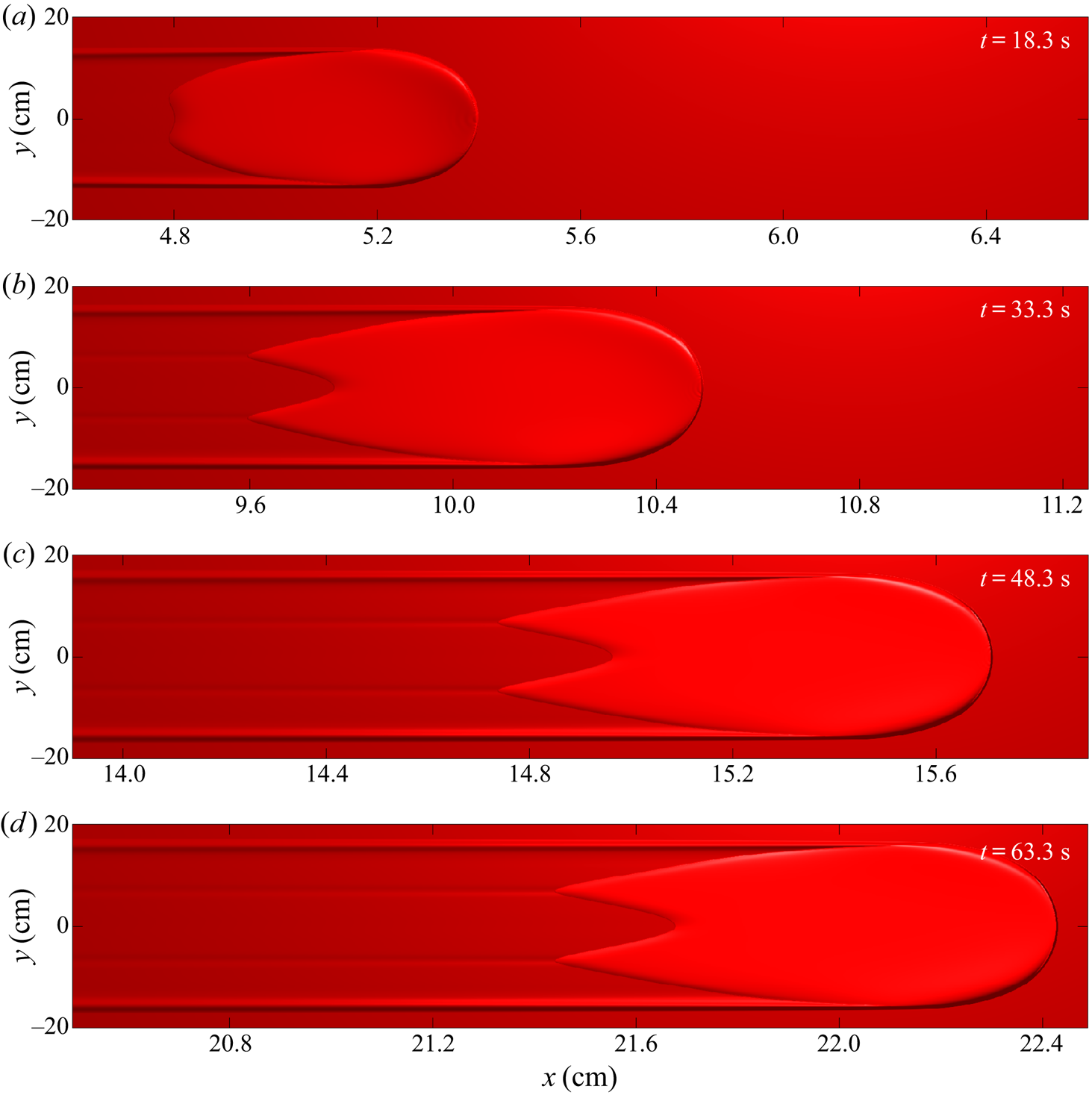
Figure 15. Travelling frame numerical simulation of a 10 ml release on a static layer of thickness  $h_0=h_{stop}(33.5^{\circ })=2.0\ \textrm {mm}$ and a slope angle of
  $\zeta =34.0^{\circ }$, shown at 15 s time intervals (a–d). An inflow of
  $h_0$ deep stationary material is imposed at the downstream boundary. The frame travels at a speed of
  $u_f = 0.31\ \textrm {m}\,\textrm {s}^{-1}$ for the first
  $20\ \textrm {s}$,
  $u_f = 0.34\ \textrm {m}\,\textrm {s}^{-1}$ for the next
  $15\ \textrm {s}$ and
  $u_f = 0.35\ \textrm {m}\,\textrm {s}^{-1}$ for the final
  $25\ \textrm {s}$, which are used to transform back to the physical
  $x$-coordinate. Surface plots of the plane viewed perpendicularly from above are coloured red, since no yellow particles remain at the times shown, and an artificial light source at the downslope end provides visualization of the three-dimensional flow thickness, as in the experiments. Mobile regions of flow with non-zero momentum appear brighter due to an increased reflectance. The growing avalanche eventually reaches a massive steady state with a double-tailed bulk head that fills almost half of the 2.0 m by 0.4 m domain. A movie showing the time-dependent evolution is available in the online supplementary material.
Further numerical simulations are carried out for 10 ml releases on various inclinations  $\zeta =34.5^{\circ }$,
  $\zeta =35.0^{\circ }$,
  $\zeta =35.5^{\circ }$ and
  $\zeta =36.0^{\circ }$ and
  $\zeta =36.5^{\circ }$ with the stationary layer thickness for each slope angle set to
  $h_0 = h_{stop}(\zeta -0.5^{\circ }) > h_{stop}(\zeta )$. Each of these initial conditions result in avalanches that grow in size as they propagate downslope by eroding more grains from the abundantly thick stationary layers than they deposit, until a large steady state is eventually reached. Relationships between the slope inclination on which the cylinder is released and the wave speeds
  $u_w$ (measured as the front speed), widths
  $W$ (between levee peaks), amplitudes
  $A$ (peak avalanche height above
  $h_0$) and mobile flow volume
  $V_m$ (the integral over non-stationary flow regions) of the resultant large steady-state avalanches are shown in figure 16. In general, the large steady-state avalanche wave speeds, widths, volumes and amplitudes are all found to decrease with increasing slope angle.
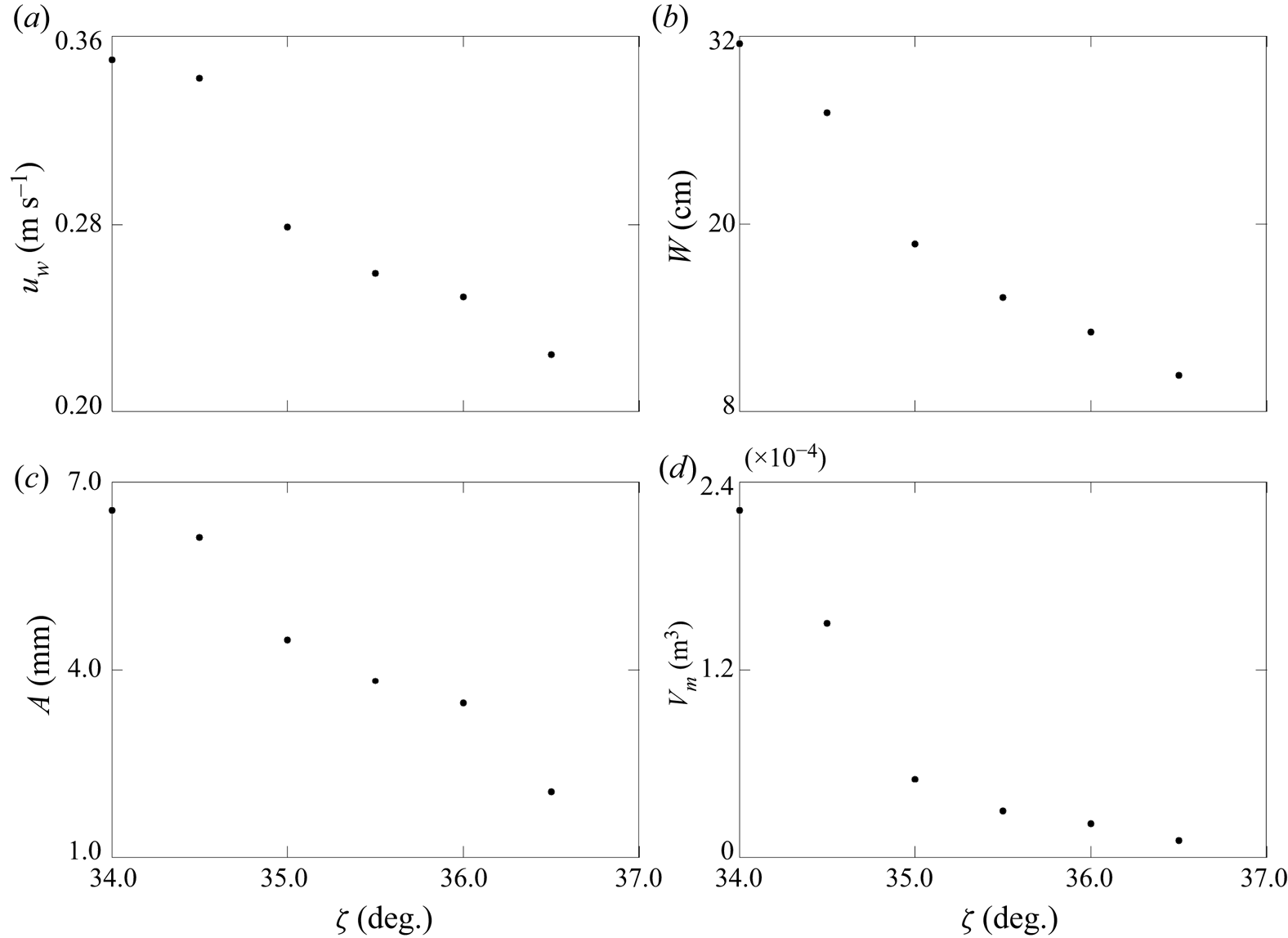
Figure 16. Large steady-state characteristics resulting from travelling frame numerical simulations of 10 ml releases on static layers of thickness  $h_0=h_{stop}(\zeta -0.5^{\circ })$ and at slope angles of
  $\zeta =34.5^{\circ }$,
  $\zeta =35.0^{\circ }$,
  $\zeta =35.5^{\circ }$ and
  $\zeta =36.0^{\circ }$ and
  $\zeta =36.5^{\circ }$. (a) Travelling wave speed, (b) leveed-channel width, (c) peak amplitude and (d) mobile flow volume are plotted (solid markers) against slope angle. All of these quantities are found to decrease with increasing slope angle.
5.3. Long distance propagation of shedding and secondary avalanches
For the shedding and secondary avalanche simulations, the computational domain consists of  $(1000,200)$ grid points in the
  $(\xi ,\upsilon )$-plane defined for the range
  $-5\ \textrm {cm} \leq \xi \leq 95\ \textrm {cm}$ and
  $-10\ \textrm {cm} \leq \upsilon \leq 10\ \textrm {cm}$. Firstly, the initial conditions are taken from the shedding avalanche simulation shown in figure 10 at
  $t_0=3.7\ \textrm {s}$, which resulted from a
  $V=10\ \textrm {ml}$ standard release (as described in § 4) of grains on a static layer of
  $h_0=h_{stop}(35.8^{\circ })=0.9\ \textrm {mm}$ depth and at a slope angle of
  $\zeta =35.8^{\circ }$. The frame speed is set to a constant speed
  $u_f = 0.17\ \textrm {m}\,\textrm {s}^{-1}$, which is used to transform back to the physical
  $x$-coordinate and the results are shown as surface plots in figure 17. It is evident that the avalanche is in fact slowly decaying, and comes to rest after travelling to
  $x\approx 2.1\ \textrm {m}$ downslope.

Figure 17. Travelling frame numerical simulation of a 10 ml release on a static layer of thickness  $h_0=h_{stop}(35.8^{\circ })=0.9\ \textrm {mm}$ and a slope angle of
  $\zeta =35.8^{\circ }$, shown at 2.0 s time intervals (a–d). An inflow of
  $h_0$ deep stationary material is imposed at the downstream boundary and the frame travels at a constant speed
  $u_f = 0.17\ \textrm {m}\,\textrm {s}^{-1}$, which is used to transform back to the physical
  $x$-coordinate. Surface plots of the plane viewed perpendicularly from above are coloured red, ignoring the yellow-particle concentration. The avalanche loses momentum after shedding mass and eventually comes to rest after travelling to
  $x\approx 2.1\ \textrm {m}$ downslope. A movie showing the time-dependent evolution is available in the online supplementary material.
Next, the initial conditions are taken from the shedding and secondary avalanche simulation shown in figure 11 at  $t_0=2.9\ \textrm {s}$, which resulted from a
  $V=20\ \textrm {ml}$ standard release of grains on a static layer of the same depth on the same slope inclination. The frame speed in this case is set to a slightly greater value of
  $u_f = 0.18\ \textrm {m}\,\textrm {s}^{-1}$ to compensate for extra momentum of the avalanche following a larger release, and which is used to transform back to the physical
  $x$-coordinate. The resultant surface plots in figure 18 show that this larger avalanche also comes to rest after travelling slightly further downslope due to this greater initial momentum, eventually coming to rest after reaching
  $x\approx 2.7\ \textrm {m}$ downslope. These results suggest that, as well as avalanches decaying when the slope angle is too shallow for them to gain momentum, a slow decay is also possible if the inclination is sufficiently steep. In such cases, the bulk flow immediately sheds an abundance of mass, and in doing so reduces its momentum below the minimum that is required to maintain flow. This result therefore suggests that not only is the avalanche behaviour sensitive to the erodible layer thickness, but also that there is only a small range of slope angles for which a steady state can prevail.
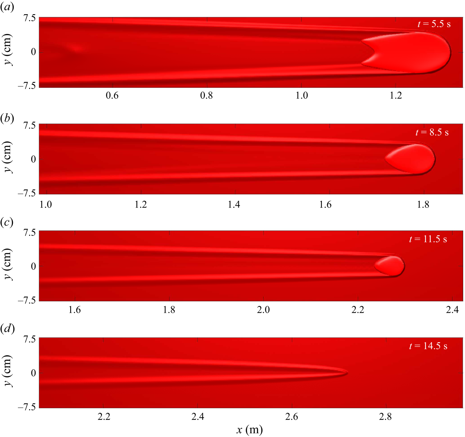
Figure 18. Travelling frame numerical simulation of a 20 ml release on a static layer of thickness  $h_0=h_{stop}(35.8^{\circ })=0.9\ \textrm {mm}$ and a slope angle of
  $\zeta =35.8$, shown at 3.0 s time intervals (a–d). An inflow of
  $h_0$ deep stationary material is imposed at the downstream boundary and the frame travels at a constant speed
 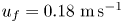 $u_f = 0.18\ \textrm {m}\,\textrm {s}^{-1}$, which is used to transform back to the physical
  $x$-coordinate. Surface plots of the plane viewed perpendicularly from above are coloured red, ignoring the yellow-particle concentration. The avalanche loses momentum after shedding mass in two chevron-shaped deposits and eventually comes to rest after travelling to
  $x\approx 2.7\ \textrm {m}$ downslope. A movie showing the time-dependent evolution is available in the online supplementary material.
6. The existence of a unique steady state
The apparently steady propagating avalanche observed both experimentally in § 2.3 and numerically in § 4.3, which propagates downslope at constant speed and deposits a leveed channel of constant width, implies the existence a steady state solution. As in the above § 5, this can be investigated numerically by using a travelling frame of reference to study the long distance propagation behaviour. This allows a much longer computational time for a steady state to be achieved than is possible on a full-size physical domain or in experiments.
The system of conservative travelling frame equations are solved numerically on a rectangular computational domain of  $(1000,200)$ grid points in the
  $(\xi ,\upsilon )$-plane defined for the range
  $0\ \textrm {cm} \leq \xi \leq 100\ \textrm {cm}$ and
  $-10\ \textrm {cm} \leq \upsilon \leq 10\ \textrm {cm}$. For each travelling frame simulation, the initial conditions are taken from a near-end state of a steady avalanche computation on a domain representing the experimental plane, after a time
  $t=t_0$ when the flow front is close to the downstream boundary.
6.1. Long distance propagation of a steady avalanche
A  $10\ \textrm {ml}$ volume of yellow grains is released on a static layer of
  $h_0=h_{stop}(34.5^{\circ })=1.4\ \textrm {mm}$ depth and at a slope angle of
  $\zeta =34.5^{\circ }$ on an experimental plane domain in the standard way, as described in § 4. The state after
  $t_0 = 3.3\ \textrm {s}$ of this computation is then imposed as the initial condition for a travelling frame simulation, with the frame speed set to
  $u_f = 0.22\ \textrm {m}\,\textrm {s}^{-1}$. The results are shown at 25 s time intervals as surface plots of the flow thickness viewed perpendicularly from above, coloured by the depth-averaged red-particle concentration
  $\bar {\phi }$ (though no yellow particles remain at the times shown) and with an artificial light source at the downslope end of the domain, in figure 19. It is clear that the apparently steady avalanche of the initial conditions does reach a genuinely steady state that maintains a constant size, speed (slightly slower than that of the frame) and leveed-channel width for the entire latter 75 s of the simulation, between panels (a,d). Thus, avalanches may propagate long distances downslope so long as they continually have the necessary conditions of slope inclination angle and erodible layer thickness to do so. In such cases, they are able to propagate by eroding stationary grains ahead of its flow front and depositing particles behind its tail in an exact delicate balance.
Figure 19. Travelling frame numerical simulation of a 10 ml release on a static layer of thickness  $h_0=h_{stop}(34.5^{\circ })=1.4\ \textrm {mm}$ and a slope angle of
  $\zeta =34.5^{\circ }$, shown at 25 s time intervals (a–d). An inflow of
  $h_0$ deep stationary material is imposed at the downstream boundary and the frame travels at a constant speed
  $u_f = 0.22\ \textrm {m}\,\textrm {s}^{-1}$, which is used to transform back to the physical
  $x$-coordinate. Surface plots of the plane viewed perpendicularly from above are coloured red, since no yellow particles remain at the times shown. The avalanche reaches a steady state and propagates for the entire 100 s simulation. A movie showing the time-dependent evolution is available in the online supplementary material.
Further evidence of this steady state is provided by the cross-slope flow thickness profiles plotted in figure 20 at 25 s time intervals. At each of the simulation times, the cross-slope profile is plotted at the downslope position  $x = x_p - 0.5\ \textrm {m}$, where
  $x_p$ is the time-dependent
  $x$-location of the maximum peak amplitude. The latter two plots show that the deposit is practically identical during the final 25 s of the simulation and that a steady state is therefore reached after a small adjustment over a long period. All of the yellow grains released from the cylinder are deposited early on, such that the steady avalanche is comprised only of red particles eroded from the static layer by
  $28.3\ \textrm {s}$ of propagation (figures 19 and 20). This confirms that the erosion-deposition process by which the avalanche propagates involves a continuous exchange of particles with the stationary substrate layer.
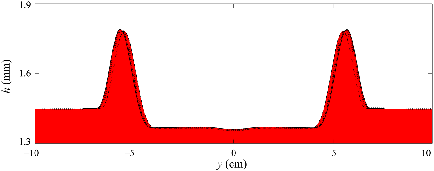
Figure 20. Travelling frame numerical simulation of a 10 ml release on a static layer of thickness 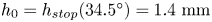 $h_0=h_{stop}(34.5^{\circ })=1.4\ \textrm {mm}$ and a slope angle of
  $\zeta =34.5^{\circ }$. Flow thickness
  $h$ is plotted against the cross-slope
  $y$-direction and filled with red colour at times
  $t = 28.3\ \textrm {s}$ (dashed black line),
  $t = 53.3\ \textrm {s}$ (dotted black line),
  $t = 78.3\ \textrm {s}$ (dash-dotted black line) and
  $t=103.3\ \textrm {s}$ (solid black line) at
  $x = x_p - 0.5\ \textrm {m}$, where
  $x_p$ is the downslope position of the peak amplitude at those times. The leveed-channel width slowly adjusts and then remains essentially unchanged in the final
  $25\ \textrm {s}$ of propagation after a steady state has been reached, which contains no yellow particles from the initial release.
It has not been previously investigated whether there exist multiple steady states corresponding to different volumes of material released for a given slope angle and erodible layer thickness. It will now be shown that changing the volume of the cylinder does not actually affect the long-time steady state solution, so long as there is sufficient material for the avalanche to propagate rather than to decay.
6.2. A unique steady state
Additional travelling frame simulations are now performed, in the same manner as above, for different volumes  $V = 8\ \textrm {ml}$, 12 ml, 15 ml and 20 ml of the standard release. The initial conditions for each are taken at times
  $t_0=3.3\ \textrm {s}$ of simulations on a domain that represents an experimental plane, inclined at a slope angle of
  $\zeta =34.5^{\circ }$ and covered with an
  $h_0=h_{stop}(34.5^{\circ })=1.4\ \textrm {mm}$ deep static erodible layer. The speed of the moving frame is set to
  $u_f = 0.22\ \textrm {m}\,\textrm {s}^{-1}$ for all of the simulations and the results, after a further 100 s has elapsed, are plotted as coloured flow thickness surfaces in figure 21 alongside the previous
  $V=10\ \textrm {ml}$ computation. Aside from small variations in the distance of propagation, due to the differing initial momentum of each cylindrical volume collapse, all of the avalanches are shown to reach exactly the same steady state as one another.
Figure 21. Travelling frame numerical simulations of (a) 8 ml, (b) 10 ml, (c) 12 ml, (d) 15 ml and (e) 20 ml releases on a static layer of thickness  $h_0=h_{stop}(34.5^{\circ })=1.4\ \textrm {mm}$ and a slope angle of
  $\zeta =34.5^{\circ }$ shown at the final simulation times
  $t=103.3$ s. An inflow of
  $h_0$ deep stationary material is imposed at the downstream boundary and the frame travels at a constant speed
  $u_f = 0.22\ \textrm {m}\,\textrm {s}^{-1}$, which is used to transform back to the physical
  $x$-coordinate. Surface plots of the plane viewed perpendicularly from above are coloured red, since no yellow particles remain at the times shown. Each volume release eventually forms an avalanche with the same steady state as one another, which only travel slightly different distances according to initial momentum. Movies showing the time-dependent evolution are available in the online supplementary material.
Cross-slope profiles for each volume release, shown at  $x = x_p - 0.5\ \textrm {m}$ downslope and times
  $t=103.3\ \textrm {s}$ in figure 22, are identical and thus confirm an equivalence of deposit thickness profile. This implies the existence of a unique steady state for avalanches that propagate downslope by undergoing a delicately balanced particle exchange with a stationary precursor layer via erosion and deposition. For a given set of suitable conditions on which a steady state avalanche can form, there is therefore an associated preferential bulk flow size and constant speed, with a corresponding leveed-channel deposit width. These attributes are likely to be dependent on the magnitude of viscosity, as they are for levees formed by self-channelizing monodisperse flows (Rocha, Johnson & Gray Reference Rocha, Johnson and Gray2019). The unique steady states are independent of the volume of material from which it is formed, provided that enough momentum is gained during an initial collapse of sufficient mass for the resultant avalanche to reach a steady state instead of abruptly coming to rest. For instance, in this flow configuration, a standard release of
  $V=5\ \textrm {ml}$ forms a decaying avalanche like those observed experimentally in § 2.1 and numerically in § 4.1, since the initial volume of grains is insufficient for a steady state to be attained.

Figure 22. Convergence of solutions from travelling frame numerical simulations of 8 ml (red lines), 10 ml (black lines), 12 ml (green lines) 15 ml (blue lines) and 20 ml (magenta lines) volume releases on a static layer of thickness  $h_0=h_{stop}(34.5^{\circ })=1.4\ \textrm {mm}$ and a slope angle of
  $\zeta =34.5^{\circ }$ shown at the final simulation times
  $t=103.3$ s. Flow thickness
  $h$ is plotted against the cross-slope
  $y$-direction for each simulation at times
  $t = 13.3\ \textrm {s}$ (dashed lines) and
  $t=103.3\ \textrm {s}$ (solid lines) at
  $x = x_p - 0.5\ \textrm {m}$, where
  $x_p$ is the downslope position of the peak amplitude at those times. The leveed-channel widths at the earlier time are different and increase with the volume of the release. At the later time, however, the widths are all equal and correspond to a unique steady state avalanche, which is independent of the volume release and is comprised entirely of red particles eroded from the substrate layer.
Note that the existence of a unique steady state contradicts the experimental observations of Viroulet et al. (Reference Viroulet, Edwards, Kokelaar and Gray2019), who found different steady state widths when varying the initial volume of releases at the same slope angle and on the same erodible layer thickness. However, their conclusions were reached based on experiments on an 80 cm long plane, over which distance the avalanches have been shown above to still be adjusting. It is reasonable to expect then, that experimental avalanches on a sufficiently long plane would also eventually reach a unique steady state, independent of the volume released.
Various steady state avalanches are also found numerically at different slope angles  $\zeta =34.2^{\circ }$,
  $\zeta =34.5^{\circ }$,
  $\zeta =34.8^{\circ }$,
  $\zeta =35.0^{\circ }$ and
  $\zeta =35.2^{\circ }$, on stationary layers of corresponding thickness
  $h_0=h_{stop}(\zeta )$. Steady states are only found to exist in this small range of inclinations
  $34.2^{\circ } \leq \zeta \leq 35.2^{\circ }$, and the relationships between the slope angle and the resulting avalanche wave speeds
  $u_w$ (measured as the front speed), widths
  $W$ (between levee peaks), amplitudes
  $A$ (peak avalanche height above
  $h_0$) and mobile flow volume
  $V_m$ (the integral over non-stationary flow regions) are shown in figure 23. Below the minimum angle for the existence of steady states, particles move more slowly on shallow inclinations. As such, the resulting avalanches are unable to gain sufficient momentum required to propagate and so they decay, as previously observed in both experiments and numerics. Above the maximum angle that steady state avalanches are found numerically, the plotted characteristic flow relationships show that avalanches become too small in amplitude and volume to maintain the necessary momentum for steady propagation. In general, the steady avalanche wave speeds, widths and amplitudes are all found to decrease linearly with increasing slope angle, while the volumes decrease quadratically, in the range of inclinations where the steady states are found to exist.
Figure 23. Steady state characteristics resulting from travelling frame numerical simulations of 10 ml releases on static layers of thickness  $h_0=h_{stop}(\zeta )$ and at slope angles of
  $\zeta =34.2^{\circ }$,
  $\zeta =34.5^{\circ }$,
  $\zeta =34.8^{\circ }$,
  $\zeta =35.0^{\circ }$ and
  $\zeta =35.2^{\circ }$. (a) Travelling wave speed, (b) leveed-channel width, (c) peak amplitude and (d) mobile flow volume are plotted (solid markers) against slope angle at simulation times
  $t=103.3\ \textrm {s}$, along with best linear (a–c) and quadratic (d) fits (solid lines) to the data. Steady states are only found to exist for slope angles
  $34.2^{\circ } \leq \zeta \leq 35.2^{\circ }$ (white regions) and not outside this range (grey regions).
The existence of a unique steady state flow regime, which has a preferential size and speed that depends only on the slope inclination and erodible layer depth, is another important discovery for application to risk assessment, since this implies that the mass of an avalanche does not necessarily depend on the volume of material that triggers it.
6.3. Transportation of particles by a steady state avalanche
The continuous erosion-deposition process by which a steady avalanche propagates is investigated further by performing a travelling frame numerical simulation in which the positions of particles that are initially located downslope of a steady avalanche front are tracked. The final time  $t=103.3\ \textrm {s}$ state for a steady avalanche resulting from a 10 ml release on an erodible layer of
  $h_0=h_{stop}(34.5^{\circ })=1.4\ \textrm {mm}$ depth and at a slope angle of
  $\zeta =34.5^{\circ }$, shown in figure 19(d), is then imposed as the initial conditions for a further travelling frame simulation with the frame speed still set to
  $u_f = 0.22\ \textrm {m}\,\textrm {s}^{-1}$. Note that the properties of the steady state avalanche are independent of the initial volume release, provided that it is sufficient to sustain its momentum, as shown above.
Three-dimensional particle tracking is initiated by randomly distributing 600 thousand particles within a cross-slope strip of the domain,  $77\ \textrm {cm} \leq \xi \leq 79\ \textrm {cm}$ and
  $0 \leq z \leq h_0$, which is immediately downslope of the avalanche front at the simulation start time
  $\hat {t}=0$. The individual positions of these yellow tracer particles are then calculated by solving (5.2a–c) concurrently with time integration of the conservation equations, as before.
The transportation of these tracer particles is shown in figure 24, where the results are plotted as flow thickness contours and yellow markers where grains are located on the free surface. Some particles are pushed around the sides of the avalanche flow front and immediately deposited in the lateral levees, while others are entrained into the bulk head. The latter type eventually resurface near the point of peak amplitude before being deposited at the rear of the avalanche, forming a double-tail structure in the center of the channel between the levees. Particles that are transported furthest are gradually deposited at the interior lateral extents of the channel walls, and the avalanche eventually contains no yellow tracers once more. This result reinforces the observation that avalanches like these propagate by continually eroding grains from the substrate layer and depositing them behind, rather than transporting the same grains in the bulk flow head.
Figure 24. Travelling frame numerical simulation of a 10 ml release on a static layer of thickness  $h_0=h_{stop}(34.5^{\circ })=1.4\ \textrm {mm}$ and a slope angle of
  $\zeta =34.5^{\circ }$, shown at 3 s time intervals (a–f). An inflow of
  $h_0$ deep stationary material is imposed at the downstream boundary and the frame travels at a constant speed
  $u_f = 0.22\ \textrm {m}\,\textrm {s}^{-1}$. Surface plots of the plane viewed perpendicularly from above are coloured red. A section of tracer particles (solid yellow markers) are inserted into the flow on the downslope side of the avalanche front, and their positions as time elapses are followed. Particles are either pushed to the sides of the flow front to form the lateral levees or are entrained by the bulk head and eventually deposited in the channel at the rear of the avalanche. A movie showing the time-dependent evolution is available in the online supplementary material.
7. Conclusions
This paper has shown that a finite release of yellow sand on a rough inclined plane covered with an erodible layer of the same material, but coloured red, triggers an avalanche whose behaviour depends on the slope angle and the substrate depth. As well as the decaying, growing and steady avalanche behaviours previously studied by Edwards et al. (Reference Edwards, Viroulet, Kokelaar and Gray2017) for flows of carborundum on a static layer of the same grains, shedding behaviours and secondary flows have also been observed here on steeper slopes when an avalanche quickly loses excess mass to adjust to a preferential size. Using two different colours of sand with identical frictional properties allows the exchange of particles, which takes place through erosion and deposition between the erodible layer and the avalanche during its propagation, to be visualized. It is evident that all of the observed avalanche types continually exchange particles with the erodible substrate as they travel downslope, such that they will eventually be composed entirely of particles originally from the stationary layer if allowed to propagate for sufficient distances. The long distance propagation behaviour of all but decaying avalanches, which travel a short distance before coming to rest, is unknown, however, since the experiments are restricted to a finite sized plane. Numerical simulations of a model replicating the experimental conditions, but in a moving frame, are therefore used to investigate the behaviour when the avalanches are allowed to propagate further.
Remarkably, given the notorious difficulty of modelling erosion-deposition problems, all of the experimentally observed avalanche behaviours can be captured in a framework that implements Edwards et al.'s (Reference Edwards, Russell, Johnson and Gray2019) basal friction rule into a two-dimensional generalization (Baker et al. Reference Baker, Barker and Gray2016) of the depth-averaged  $\mu (I)$-rheology (Gray & Edwards Reference Gray and Edwards2014). The flow is assumed to be either static or mobile throughout its entire depth at each point instead of explicitly resolving the interface between stationary and moving grains in the vertical direction, which is a crude yet reasonable approximation for the shallow erodible layers studied here. The extended rough bed friction rule (3.7)–(3.9), which instead essentially determines which regions are in motion, has been modified from Pouliquen & Forterre's (Reference Pouliquen and Forterre2002) formulation to transition between dynamic and static states more gradually, with a
  $\kappa =1$ interpolation power, and at a higher than normal, constant slope-angle independent Froude number
  $\beta _*$. These modifications provide greater stability to static layers in the hysteretic region
  $h_{stop} < h < h_{start}$ as well as correctly predicting the experimental deposit depth
  $h_{stop}$ left by a steady uniform flow over the whole range of permissible slope angles (Edwards et al. Reference Edwards, Russell, Johnson and Gray2019), respectively. A result of this is that the model is able to capture the novel shedding and secondary avalanche behaviours, in particular, which were observed here in experiments. Equations of motion for individual particles are solved simultaneously with the depth-averaged model, which qualitatively reproduces the particle exchange observed between an erodible layer and an avalanche that will eventually contain only grains that have been entrained from the substrate.
The long distance propagation behaviour of growing, shedding and apparently steady avalanches was investigated by performing numerical simulations in a frame of reference that moved at the wave speed of the bulk flow. The results showed that growing avalanches are able to eventually reach massive steady states by entraining much more material than they deposit until a limiting size is reached. Shedding avalanches were found to slowly decay after first travelling some distance downslope, due to a loss of momentum following the initial readjustment of mass. Finally, it was shown that a genuine steady state can be achieved given suitable conditions are provided indefinitely, with an avalanche able to propagate for more than 100 s by undergoing a perfectly balanced erosion-deposition process. The motion of particle tracers initially located in a strip across the stationary layer ahead of this steady state corroborate the previous findings that an avalanche propagates on an erodible layer by continually exchanging grains with it and the bulk flow. Furthermore, different volume releases for the same slope angle and erodible layer depth all eventually converge to the same unique steady state, unless there was insufficient mass and therefore momentum to prevent decay, implying a preferential avalanche size and speed exists. Despite the model for erosion and deposition used here being relatively simple, these findings may all have important consequences for mitigation of risk posed by various types of erosive geophysical mass flows, since the growth of snow avalanches through frontal entrainment (Sovilla et al. Reference Sovilla, Sommavilla and Tomaselli2001; Sovilla & Bartelt Reference Sovilla and Bartelt2002; Sovilla et al. Reference Sovilla, Burlando and Bartelt2006) is strongly dependent on the net erosion-deposition rate and the existence of an easily erodible layer can significantly enhance run-out distances (Mangeney et al. Reference Mangeney, Roche, Hungr, Mangold, Faccanoni and Lucas2010; Iverson et al. Reference Iverson, Reid, Logan, LaHusen, Godt and Griswold2011).
Supplementary movies
Supplementary movies are available at https://doi.org/10.1017/jfm.2021.34 and https://doi.org/10.17632/s8c6dws3s4.1.
Acknowledgements
J.M.N.T.G. is a Royal Society Wolfson Research Merit Award holder (WM150058) and an EPSRC Established Career Fellow (EP/M022447/1). All research data supporting this publication are directly available within this publication.
Funding
This research was supported by NERC grants NE/E003206/1 and NE/K003011/1 as well as EPSRC grants EP/I019189/1, EP/K00428X/1 and EP/M022447/1.
Declaration of interests
The authors report no conflict of interest.


 Open access