


1. Introduction
Turbulence modulation by inertial particles represents a challenging multiscale problem (Soldati & Marchioli Reference Soldati and Marchioli2009; Balachandar & Eaton Reference Balachandar and Eaton2010), whose full understanding would impact on a better comprehension of natural phenomena (Woods Reference Woods2010; Fu et al. Reference Fu, Li, Lubow, Li and Liang2014), and technological applications ranging from industrial (Jenny, Roekaerts & Beishuizen Reference Jenny, Roekaerts and Beishuizen2012; Capecelatro, Pepiot & Desjardins Reference Capecelatro, Pepiot and Desjardins2014) to medical applications (Kleinstreuer & Zhang Reference Kleinstreuer and Zhang2010).
Besides its relatively simple geometrical configuration, the turbulent flow in a channel still represents a paradigmatic problem in multiphase flows; see Marchioli, Picciotto & Soldati (Reference Marchioli, Picciotto and Soldati2007), Sardina et al. (Reference Sardina, Schlatter, Brandt, Picano and Casciola2012) and Fong, Amili & Coletti (Reference Fong, Amili and Coletti2019). One of the major issues in wall turbulence is whether or not the presence of solid particles can modify the flow friction at the wall, and the overall structure of the turbulent fluctuations. Indeed, there are numerical studies that report drag reduction by particles (Vreman Reference Vreman2007; Zhao, Andersson & Gillissen Reference Zhao, Andersson and Gillissen2010), while others report its increase, both numerically (Pan & Banerjee Reference Pan and Banerjee1997; Costa, Brandt & Picano Reference Costa, Brandt and Picano2020, Reference Costa, Brandt and Picano2021) and experimentally (Righetti & Romano Reference Righetti and Romano2004; Li et al. Reference Li, Wang, Liu, Chen and Zheng2012).
The lack of a clear answer can be ascribed to two main reasons. The first is represented by the multiscale interaction between turbulence and inertial particles that can be parametrised in terms of additional dimensionless parameters, i.e. the particle Reynolds number, the particle-to-fluid density ratio, the particle-to-fluid response time (i.e. the Stokes number), and the volume fraction of the suspensions; see Elgobashi (Reference Elgobashi2006). At least a four-dimensional parameter space should be explored with experiments and/or numerical simulations to characterise the turbulence modification. The second reason concerns the different numerical approaches describing with different grades of accuracy the fluid–particle interaction; see e.g. the review by Brandt & Coletti (Reference Brandt and Coletti2022). Usually, a very accurate description of the fluid–particle interaction goes along with a tremendous computational cost. Resolved particle simulations have been applied to study the effect of almost neutrally buoyant suspensions and the modulation of wall turbulence of one specific particle population. However, when a wider range of the parameter space is spanned, the intrinsic scale separation calls for modelling the fluid–particle interaction in order to reduce the computational cost. When the flow past each particle is not actually resolved, the major interaction between the fluid and the point-particles consists of the momentum exchange (two-way coupling regime).
In the limit of small particle Reynolds number, and dilute volume fractions, the particle-source in cell method (Crowe, Sharma & Stock Reference Crowe, Sharma and Stock1977) has been the first approach designed to capture the interphase momentum exchange. Since (Crowe et al. Reference Crowe, Sharma and Stock1977), many alternative and more accurate approaches have been conceived – see, for instance, Garg et al. (Reference Garg, Narayanan, Lakehal and Subramaniam2007), Horwitz & Mani (Reference Horwitz and Mani2016), Pakseresht, Esmaily & Apte (Reference Pakseresht, Esmaily and Apte2020) and Evrard, Denner & van Wachem (Reference Evrard, Denner and van Wachem2021) – in the context of Euler–Lagrangian simulations. Other authors filtered the fluid equations on the scale of the particle accounting for excluded volume effects, and the related subgrid stresses on the fluid (Capecelatro & Desjardins Reference Capecelatro and Desjardins2013; Ireland & Desjardins Reference Ireland and Desjardins2017). In the force coupling method (Maxey & Patel Reference Maxey and Patel2001; Lomholt & Maxey Reference Lomholt and Maxey2003; Yeo & Maxey Reference Yeo and Maxey2010) and the pairwise interaction extended point-particle method (Akiki, Jackson & Balachandar Reference Akiki, Jackson and Balachandar2017a; Akiki, Moore & Balachandar Reference Akiki, Moore and Balachandar2017b), the authors evaluated the local disturbance produced by the particles by solving a steady Stokes flow. In the exact regularised point-particle (ERPP) method (Gualtieri et al. Reference Gualtieri, Picano, Sardina and Casciola2015; Battista et al. Reference Battista, Mollicone, Gualtieri, Messina and Casciola2019), and in the work by Balachandar, Liu & Lakhote (Reference Balachandar, Liu and Lakhote2019), the particle disturbance was modelled exploiting unsteady Stokes solutions. Other related approaches adopt regularisation procedures based on nonlinear diffusion processes; see Poustis et al. (Reference Poustis, Senoner, Zuzio and Villedieu2019). All the above methods aimed to retrieve in a somehow lumped way the boundary condition that was killed when the particles were modelled as point masses (see Prosperetti Reference Prosperetti2015), still preserving an accurate and physically reliable description of the fluid–particle interaction. The ERPP method reproduces faithfully the momentum exchange between small particles and the carrier phase, and given its computational efficiency, it can be used to explore a wide range of the parameter space where turbulence modulation occurs at different grades.
This paper addresses the turbulence modulation in the range of Stokes number  $St_+ \in [2,80]$, and of particle-to-fluid density ratio $\rho _p/\rho _f \in [90,5760]$ at a fixed mass loading $\phi =0.4$. In this region of the parameter space, the overall friction drag is either increased or left unaltered. This behaviour is explained in terms of the particles’ additional momentum transfer towards the wall, i.e. the particles’ extra stress, and in terms of the modification of the turbulent kinetic energy (TKE) budget. As discussed by Capecelatro, Desjardins & Fox (Reference Capecelatro, Desjardins and Fox2018), there exist regimes where TKE production due to the Reynolds shear stress (shear production) is overwhelmed by the particle feedback term (particle production). In homogeneous flows (Richter Reference Richter2015; Gualtieri, Battista & Casciola Reference Gualtieri, Battista and Casciola2017), this results in the increase of the fluid dissipation rate at the scales where additional kinetic energy is produced. In inhomogeneous conditions, however, these mechanisms originate a spatial energy flux. Indeed, in regimes where a strong increase of the friction drag is observed, the particle production term turns out to be the largest one and is localised near the wall. The excess of TKE produced by the particles is not locally dissipated and triggers an intense spatial energy flux towards the wall, where ultimately the energy is dissipated by the viscosity. This behaviour explains the increase of the friction drag and the concurrent increase of velocity fluctuations that are observed in the viscous sublayer in the presence of two-way coupling effects.
The paper is organised as follows. Section 2 summarises briefly the numerical approach based on the ERPP model, and discusses the simulations’ parameters. Section 3 first documents the turbulence modulation and then explain it in terms of the alteration of the stress and TKE balances. Section 4 draws the main conclusions of the study.
2. Particle-laden turbulent channel flow
The dimensionless Navier–Stokes equations for a divergence-free velocity field,
 \begin{equation}
\left.\begin{array}{cc@{}} \boldsymbol{\nabla}
\boldsymbol{\cdot} \boldsymbol{u} = 0, \\
\displaystyle \dfrac{\partial \boldsymbol{u}}{\partial t} +
\boldsymbol{\nabla} \boldsymbol{\cdot} \left(\boldsymbol{u}
\otimes \boldsymbol{u}\right) ={-} \left.\dfrac{{{\rm d} p}}{{\rm d}\kern0.7pt x}\right|_0 \boldsymbol{e}_x -
\boldsymbol{\nabla} p + \dfrac{1}{Re_b}\,\nabla^2
\boldsymbol{u} + \boldsymbol{f}, \end{array}\!\!\!\right\} \end{equation}
\begin{equation}
\left.\begin{array}{cc@{}} \boldsymbol{\nabla}
\boldsymbol{\cdot} \boldsymbol{u} = 0, \\
\displaystyle \dfrac{\partial \boldsymbol{u}}{\partial t} +
\boldsymbol{\nabla} \boldsymbol{\cdot} \left(\boldsymbol{u}
\otimes \boldsymbol{u}\right) ={-} \left.\dfrac{{{\rm d} p}}{{\rm d}\kern0.7pt x}\right|_0 \boldsymbol{e}_x -
\boldsymbol{\nabla} p + \dfrac{1}{Re_b}\,\nabla^2
\boldsymbol{u} + \boldsymbol{f}, \end{array}\!\!\!\right\} \end{equation}
are solved in the domain  $\mathcal {D} = [0, 4{\rm \pi} ] \times [0, 2{\rm \pi} ] \times [0,2]$ in the streamwise ( $x$), spanwise ( $y$) and wall-normal ( $z$) directions, respectively. Periodic boundary conditions are applied along the streamwise and spanwise directions, whilst no-slip boundary conditions are enforced at the channel's top and bottom walls. The flow is sustained by a constant mean pressure gradient ${\rm d} p/{{\rm d}\kern0.7pt x}|_0$ applied in the direction of the streamwise unit vector $\boldsymbol {e}_x$. The reference quantities are the fluid density $\rho _f$, the channel half-height $h$, the bulk velocity of the reference uncoupled case (no back-reaction on the fluid) $U_{b,0} = Q_0/(2h)$, where $Q_0$ is the flow rate per unit length, and the fluid viscosity $\mu$. It follows that the Reynolds number is $Re_b = \rho _f U_{b,0} h/\mu$. In (2.1), field $\boldsymbol {f}$ represents the particle feedback on the fluid as modelled by the ERPP approach, namely
 \begin{equation}
\boldsymbol{f}(\boldsymbol{x},t)
={-}\sum_{p=1}^{N_p}\boldsymbol{D}_p(t-\epsilon) g[
\boldsymbol{x}-\boldsymbol{x}_p(t-\epsilon),\epsilon]
+\tilde{\boldsymbol{D}}_p(t-\epsilon) g[
\boldsymbol{x}-\tilde{\boldsymbol{x}}_p(t-\epsilon),\epsilon ],
\end{equation}
\begin{equation}
\boldsymbol{f}(\boldsymbol{x},t)
={-}\sum_{p=1}^{N_p}\boldsymbol{D}_p(t-\epsilon) g[
\boldsymbol{x}-\boldsymbol{x}_p(t-\epsilon),\epsilon]
+\tilde{\boldsymbol{D}}_p(t-\epsilon) g[
\boldsymbol{x}-\tilde{\boldsymbol{x}}_p(t-\epsilon),\epsilon ],
\end{equation}
where the sum encompasses all  $N_p$ particles. The dimensionless drag force on the $p$th particle is ${\boldsymbol {D}}_p = 3 {\rm \pi}d_p/Re_b\,(\hat {\boldsymbol {u}}|_p - \boldsymbol {v}_p)$, where $d_p$ is the dimensionless particle diameter, $\boldsymbol {v}_p$ is the particle velocity, and $\hat {\boldsymbol {u}}|_p = \hat {\boldsymbol {u}}[\boldsymbol {x}_p(t),t]$ is the fluid velocity at the particle position $\boldsymbol {x}_p(t)$ deprived by the particle self-disturbance, i.e. the field that accounts for the turbulent background velocity and for the disturbance of all particles except the $p$th. This field is evaluated by summing the contributions of all the particles and by successively removing the particle self-disturbance that, in the context of the ERPP approach, is known in a closed analytical form.
In (2.2), the variables with a tilde denote quantities about the image particles obtained by reflection with respect to the wall according to  $\tilde {\boldsymbol {x}}^{{\rm \pi} }_p=\boldsymbol {x}^{{\rm \pi} }_p$, $\tilde {x}^{n}_p=-x^{n}_p$, $\tilde {\boldsymbol {D}}^{{\rm \pi} }_p=\boldsymbol {D}^{{\rm \pi} }_p$, $\tilde {D}^{n}_p=-D^{n}_p$, where the superscripts ${{\rm \pi} }$ and $n$ denote the coordinates along the tangent plane and the wall-normal direction, respectively. The image particle is a feature of the ERPP approach to account for the particle feedback in presence of solid boundaries. Both the current time $t$ and the regularisation time scale $\epsilon _R$ are made dimensionless with $h/U_{b,0}$, namely $\epsilon = \epsilon _R U_{b,0}/h$. In the ERPP approach, the regularisation of the singular feedback force field caused by the particles in the fluid is achieved by exploiting the disturbance vorticity that each particle generates when subjected to force ${\boldsymbol {D}}_p$. The disturbance vorticity is consistently regularised by the fluid viscosity, and its ‘regular’ counterpart forces the Navier–Stokes equations via the field $\boldsymbol {f}(\boldsymbol {x},t)$ in (2.2). The delay time scale $\epsilon$ represents the time required by the vorticity generated by the particles to diffuse up to the grid size. It turns out that the Dirac delta functions that localise the force on the fluid at the particle position are turned on a physical ground into Gaussian functions, i.e. $g[ \boldsymbol {x}-\boldsymbol {x}_p(t-\epsilon ), \epsilon ]$, centred at the delayed particle position $\boldsymbol {x}_p(t-\epsilon )$ with variance given by the regularisation time scale $\epsilon$; see e.g. Gualtieri et al. (Reference Gualtieri, Picano, Sardina and Casciola2015) and Battista et al. (Reference Battista, Mollicone, Gualtieri, Messina and Casciola2019) for a more detailed description of the method.
Equations (2.1) are solved in Cartesian coordinates using an in-house developed code that exploits a hybrid MPI-GPUs parallelisation. Chorin's projection method (Chorin Reference Chorin1968) is used to enforce the divergence-free constraint imposed by the mass balance. Both convective and diffusive terms are discretised in space by second-order finite differences on a staggered grid, and are integrated explicitly in time using a third-order, four-stage, low-storage Runge–Kutta method.
Inner or wall units are provided by the viscous length  $\ell _*=\nu /u_*$ (where $\nu =\mu /\rho _f$ is the kinematic viscosity) and the friction velocity $u_*=\sqrt {\tau _w/\rho _f}$ (where $\tau _w$ is the average wall shear stress). The wall-normal distance in inner units is denoted as $z_+ = z/\ell _*$, and the friction Reynolds number is $Re_* = u_* h / \nu$. All the simulations are performed with the same friction Reynolds number $Re_*=185$. The bulk Reynolds number of the reference uncoupled case (no particle back-reaction) is $Re_b=2890$. The discretisation grid is uniformly spaced in the streamwise and spanwise directions, while it is stretched along the wall-normal direction. The number of grid points and the grid spacing are reported in table 1.
Table 1. All simulations are performed with the same mean pressure gradient corresponding to a friction Reynolds number  $Re_*=185$ and a bulk Reynolds number for the reference uncoupled case (one-way coupling, no back-reaction) $Re_b=2890$. The grid resolution is $N_x \times N_y \times N_z$ in the dimensionless domain $\mathcal {D} = [0, 4{\rm \pi} ] \times [0, 2{\rm \pi} ] \times [0,2]$. The grid spacing is uniform in the streamwise and spanwise directions corresponding to ${\rm \Delta} x_+={\rm \Delta} y_+=3$, ${\rm \Delta} x_+={\rm \Delta} y_+=2$ and ${\rm \Delta} x_+={\rm \Delta} y_+=1.5$ for the different grids. In the wall-normal direction, the grid is stretched corresponding to minimum spacing ${\rm \Delta} z_+|_w = 0.2$ at the wall and ${\rm \Delta} z_+|_0=3$ at the centreline. In all the simulations, the mass loading is $\phi =0.4$. Here, $\rho _p/\rho _f$ is the particle-to-fluid density ratio, $St_+=\tau _p/\tau _*$ is the Stokes number in wall units, $d_p^+$ is the particle diameter in wall units, and $N_p$ is the number of particles.

Concerning the disperse phase, at a relatively large particle-to-fluid density ratio  $\rho _p/\rho _f$, the only relevant hydrodynamic force acting on the particles is the Stokes drag; see Gatignol (Reference Gatignol1983) and Maxey & Riley (Reference Maxey and Riley1983). Newton's equations for the particles read
 \begin{equation}
\left.\begin{array}{cc@{}} \displaystyle \dfrac{{\rm
d}\boldsymbol{x}_p}{{\rm d} t}= \boldsymbol{v}_p,
\\ \displaystyle \dfrac{{\rm d}
\boldsymbol{v}_p}{{\rm d} t}= \dfrac{1}{St_b}
(\hat{\boldsymbol{u}}|_p - \boldsymbol{v}_p),
\end{array}\!\!\!\right\} \end{equation}
\begin{equation}
\left.\begin{array}{cc@{}} \displaystyle \dfrac{{\rm
d}\boldsymbol{x}_p}{{\rm d} t}= \boldsymbol{v}_p,
\\ \displaystyle \dfrac{{\rm d}
\boldsymbol{v}_p}{{\rm d} t}= \dfrac{1}{St_b}
(\hat{\boldsymbol{u}}|_p - \boldsymbol{v}_p),
\end{array}\!\!\!\right\} \end{equation}
where the bulk Stokes number is  $St_b = \tau _p/\tau _0 = Re_b\,\rho _p/ (18 \rho _f) (d_p / h)^2$, with ${\tau _0 = h / U_{b,0}}$, and $\tau _p$ the particle relaxation time. Equations (2.3) are integrated in time with the same four-stage, low-storage Runge–Kutta method used for the carrier phase. A purely elastic bounce is implemented at the channel's top and bottom walls. In some of the cases listed in table 1, namely for the largest Stokes numbers ( $St_+=40, 80$) and for the relatively smaller density ratio ( $\rho _p/\rho _f=90$), companion simulations that included the Faxén correction (Gatignol Reference Gatignol1983) were performed, showing inappreciable effects on the results, and they will not be discussed further here.
The dynamics of the two-way coupled system for small particle Reynolds number and dilute suspensions is controlled by a set of four dimensionless parameters, as it follows from the application of the Buckingham theorem, namely  $\{Re_*;\ St_+;\ \rho _p/\rho _f;\ N_p\}$, where $N_p$ is the total number of particles in the flow domain $\mathcal {D}$, and the inner-scale Stokes number is defined as $St_+=\tau _p/\tau _* = St_b\,Re_*^2/Re_b$, with $\tau _*= \ell _*/u_*$ the friction time scale. However, $N_p$ is a quantity that is difficult to determine experimentally. In contrast, the total mass of the disperse phase can be measured easily by a weight balance. Hence $N_p$ can be replaced by the mass loading $\phi =N_p \rho _p V_p / \rho _f V_f = (\rho _p / \rho _f) N_p (d_p/h)^3 /(96 {\rm \pi})$, where $V_p$ is the volume of the particle, and $V_f$ is the volume of the fluid in the domain $\mathcal {D}$; see e.g. Elgobashi (Reference Elgobashi2006) and Balachandar & Eaton (Reference Balachandar and Eaton2010).
A summary of the dataset is listed in table 1. In all the simulations, the friction Reynolds number  $Re_*$ is fixed (same pressure drop), implying that the actual flow rate $Q= 2h U_b$ follows as a consequence of the fluid–particle momentum exchange. The simulation plan is designed to assess in a systematic way the role of the particle Stokes number and of the particle-to-fluid density ratio on the turbulence modification at fixed mass loading $\phi =0.4$. For this purpose, the simulations are divided into two groups. In the first set of simulations, the Stokes number is changed at a fixed density ratio. The second set addresses the effect of the density ratio at fixed Stokes number. The mass loading is maintained constant by consistently adjusting the particle number $N_p$ to compensate for the increase of the mass of each particle when the density ratio and/or the Stokes number are varied. The choice of the present parameters rules out the role of gravity in the dynamics of the particles. Indeed, the ratio between the particle terminal velocity $v_t$ in a quiescent fluid and the bulk velocity can be expressed by $v_t/U_b = St_b / Fr_b^2$, where $Fr_b = U_b / \sqrt {g h}$ is the Froude number. In realistic conditions, i.e. in an actual experiment of air flowing in a channel of half-height $h=1$ cm at the present value of the bulk Reynolds number, it turns out that $v_t/U_b \simeq 0.04$ in the worst scenario, i.e. for the particle population at $St_+=80$.
3. Results
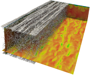
The instantaneous channel flow configuration laden with the particle population at  $St_+=10$ is reported in figure 1. Figure 1(a) pertains to the one-way coupling regime, and figure 1(b) pertains to the corresponding two-way coupling regime. The contour plot represents the fluid velocity magnitude normalised with the bulk velocity of the corresponding case. In the one-way regime, the fluid velocity is characterised by the presence of the ordered low- and high-speed streaks, whilst in the two-way regime, even though the streaky structure of the velocity field is still apparent, the spatial order is clearly altered. A related effect consists of the modification of the particle distribution. Indeed, ordered clusters are evident in figure 1(a), while they are hardly appreciable in figure 1(b). The analysis of the instantaneous flow configuration denotes an appreciable turbulence modification that is quantified and detailed below in terms of statistical observables.

Figure 1. Instantaneous configuration of the particle-laden flow in (a) the one-way coupling, and (b) the two-way coupling. The contour plot represents the velocity magnitude normalised with the bulk velocities of the corresponding cases,  $|\boldsymbol {u}|$. The particle population at $St_+=10$ is represented in both images (half of the domain is represented for the sake of clarity).
3.1. Mean flow and friction coefficient
The mean velocity profile is plotted in figure 2 for some selected relevant cases of table 1. Figures 2(a,b) show the effect of the Stokes number at a fixed density ratio in the semi-log scale and in the linear scale, respectively, the latter to better appreciate the modification of the flow rate. Particles with the largest  $St_+$, e.g. $St_+=80$, have a small, though measurable, effect on the mean velocity profile that approaches the curve of the one-way coupling regime. When the Stokes number is decreased, the interphase momentum coupling becomes more effective, and the ensuing velocity profile departs from the reference data of the one-way coupled simulation. All the data show a sensible reduction of the flow speed that occurs up to the smallest Stokes number considered, $St_+=2$. By increasing the density ratio up to $\rho _p/\rho _f=5760$ at a fixed Stokes number, the effect of the particles always results in a depletion of the velocity profile; see figures 2(c,d). Note that the depletion of the flow speed becomes progressively weaker, being the velocity profile for the case $\rho _p/\rho _f=5760$ almost superimposed on the reference Newtonian case. This suggests a relevant role of the particle-to-fluid density ratio that must be taken into account when comparing different studies and flow configurations.

Figure 2. Mean streamwise velocity  $U_x=\langle u \rangle$ versus the wall-normal distance $z$. (a,c) Data normalised with internal units, $U_x^+=U_x/u_*$ against $z_+=z/\ell _*$. (b,d) Data normalised with external units, $U_x/U_{b,0}$ against $z/h$. (a,b) Data at $\rho _p/\rho _f=180$ and $\phi =0.4$ for different Stokes numbers. (c,d) Data at fixed mass load $\phi =0.4$ and Stokes number $St_+=10$ for different density ratios. The solid black line in all plots is the mean velocity profile in the one-way coupling regime. In (a,c), the log law with $k=0.39$ and $A=6$ (dash-dotted line), and the viscous scaling $U_x^+=z_+$ (dotted line), are reported.
All the data reported in figure 2 indicate that the effect of the particles, at least in the range of parameters considered in this study, goes always in the direction of reducing the flow speed for a prescribed pressure gradient. This means that the laden flow experiences a larger friction drag than the unladen case. Figure 3 shows the ratio between the friction coefficient  $C_f= 2 \tau _w/ (\rho _f U_b^2)$ and the friction coefficient of the reference uncoupled simulation $C_{f,0}= 2 \tau _w/ (\rho _f U_{b,0}^2)$. At large Stokes numbers, the ratio $C_f/C_{f,0}$ approaches a plateau; at intermediate Stokes numbers, a rapid increase of $C_f/C_{f,0}$ is measured when decreasing $St_+$; and at relatively smaller Stokes numbers, the increase of $C_f/C_{f,0}$ is weaker though still clear. For all the values of the particle-to-fluid density ratio, the drag result is always larger than the corresponding value measured in the uncoupled case. Indeed, $C_f/C_{f,0}$ starts constant, decreases with increasing particle-to-fluid density ratios to saturate eventually at very large values of $\rho _p/\rho _f$, being always above 1.

Figure 3. The friction coefficient  $C_f$ normalised with the friction coefficient $C_{f,0}$ in the one-way coupling regime (no back-reaction). Data are plotted versus the Stokes number $St_+$ for the dataset at a fixed density ratio $\rho _p/\rho _f=180$ (bottom $x$-axis, red circles), and versus the density ratio $\rho _p/\rho _f$ for the dataset at fixed Stokes number $St_+=10$ (top $x$-axis, blue triangles).
The particle average distribution is presented in figure 4 as a function of the wall-normal distance. The particle concentration is defined as  $C(z) = (\langle n_p \rangle /{\rm \Delta} V_x)/(N_p/V_f)$, where $\langle n_p \rangle$ is the average number of particles in a cylindrical shell of volume ${\rm \Delta} V_z=L_x \times L_y \times \varDelta _z$ placed at distance $z$ from the wall, and $N_p$ is the total number of particles in the fluid domain $V_f$. The normalisation is chosen such that $C=1$ when the particles are distributed homogeneously throughout the fluid domain. Figure 4(a) documents the effect of the Stokes number, and figure 4(b) the effect of the density ratio. Note that particles cannot lie in a wall layer as thick as their radius.

Figure 4. Mean particle concentration versus wall normal distance  $z_+=z/\ell _*$. (a) Data at fixed $\rho _p/\rho _f=180$ and $\phi =0.4$ for different Stokes numbers. (b) Data at fixed $\phi =0.4$ and $St_+=10$ for different density ratios. The solid lines correspond to the two-way coupling regime; the dashed colour-matched lines correspond to the one-way coupling regime.
Concerning the effect of the Stokes number, the particle feedback modifies the particle concentration with respect to the uncoupled case only for the populations at  $St_+=2$ and $St_+=10$. At higher Stokes number ( $St_+=80$), the particles are still unevenly distributed across the flow domain, but the difference between the one-way and two-way coupled simulations is less apparent. It turns out that the particle accumulation near the wall is not necessarily the only precursor for turbulence modification. Figure 4(b) addresses the effect of the density ratio. Note that all three two-way coupled cases correspond to a single one-way couple case since in the latter, only the Stokes number matters. These results prove that $\rho _p/\rho _f$ is a crucial parameter in two-way coupled particle-laden flows, and that most of our understanding that is based on one-way coupled simulations must be reconsidered since the particle-to-fluid density ratio does not enter the uncoupled case dynamics.
3.2. Turbulent fluctuations
The mean streamwise velocity fluctuation profile is shown in figure 5. Figure 5(a) addresses the role of the Stokes number, and figure 5(b) addresses the role of the density ratio. The striking effect observed in the two-way coupling regime consists of the modification of turbulent fluctuations near the wall. Particles at large Stokes numbers  $St_+=80$ and $20$ deplete the peak intensity in the buffer layer and the lower part of the log layer. Besides the depletion in the buffer region, the particle at $St_+=10$ starts augmenting the fluctuations in the viscous sublayer. When the Stokes number is further decreased (see cases $St_+ \in [2,5]$), a new peak of velocity fluctuations appears definitively in the viscous sublayer. Concerning the effect of the density ratio (figure 5b), the fluctuations in the viscous sublayer are augmented, while the reduction of the intensity peak in the buffer region is relevant up to $\rho _p/\rho _f=1440$. In the highest density ratio $\rho _p/\rho _f=5760$ case, the viscous sublayer is unaltered, while the peak of the fluctuations is still depleted in the buffer region.

Figure 5. Mean streamwise velocity fluctuation  $\langle u^{\prime 2}_x \rangle _+= \langle u^{\prime 2}_x \rangle / u_*^2$ versus wall-normal distance $z_+=z/\ell _*$. (a) Data at fixed $\rho _p/\rho _f=180$ and $\phi =0.4$ for different Stokes numbers. (b) Data at fixed $\phi =0.4$ and $St_+=10$ for different density ratios. The solid black line in all plots corresponds to the one-way coupling regime.
Figure 6 presents the wall-normal mean velocity fluctuation profile. The two-way coupling effects are again striking in the near-wall region, where a clean peak is observed in the viscous sublayer for all the particle populations except for the case at  $St_+=80$ where, instead, fluctuations are depleted across the entire channel height. The increase of the wall-normal velocity fluctuations is particularly evident for the populations at relatively small Stokes number, i.e. $St_+ \in [2,5]$. Similar behaviour is observed for cases at different density ratios (see figure 6b), where the fluctuations approach the data of the one-way coupling regime only for the case at $\rho _p/\rho _f=5760$.

Figure 6. Mean wall-normal velocity fluctuation  $\langle u^{\prime 2}_z \rangle _+= \langle u^{\prime 2}_z \rangle / u_*^2$ versus wall-normal distance $z_+=z/\ell _*$. (a) Data at fixed $\rho _p/\rho _f=180$ and $\phi =0.4$ for different Stokes numbers. (b) Data at fixed $\phi =0.4$ and $St_+=10$ for different density ratios. The solid black line in all plots corresponds to the one-way coupling regime.
Figure 7 shows Reynolds shear stress profile modification due to the particle presence. The Reynolds stresses are reduced in the log region and in the buffer region, to be increased significantly in the viscous sublayer except for the population at  $St_+=80$. Similar behaviour is observed when the density ratio is changed.

Figure 7. Mean Reynolds shear stress profile  $\langle u^{\prime }_x u^{\prime }_z\rangle _+= \langle u^{\prime }_x u^{\prime }_z\rangle / u_*^2$ versus wall-normal distance $z_+=z/\ell _*$. (a) Data at fixed $\rho _p/\rho _f=180$ and $\phi =0.4$ for different Stokes numbers. (b) Data at fixed $\phi =0.4$ and $St_+=10$ for different density ratios. The solid black line in all plots corresponds to the one-way coupling regime.
The augmentation of the Reynolds shear stresses close to the wall indicates an increase in the momentum transfer towards the wall due to turbulent fluctuations. The turbulent fluctuations in the viscous sublayer are augmented along both the streamwise and wall-normal directions, with also an alteration of the off-diagonal components of the stresses. One can figure out that when fast particles coming from the channel bulk approach the wall, due to their inertia, they have streamwise and wall-normal velocities much different to those of the surrounding fluid. The same happens for slow particles that from the near-wall region migrate towards the centre of the channel. It follows a large slip velocity between particles and fluid, resulting in an intense and localised momentum exchange that manifests as a large increment of fluctuations. This point is investigated more deeply by addressing stress balance.
3.3. Stress balance
The mean streamwise momentum balance,
 \begin{equation} \frac{\partial}{\partial z} \left[\mu\,\frac{\partial U_x}{\partial z} -\rho_f \langle u_x^\prime u_z^\prime \rangle+ \tau_e \right] = \left.\frac{{\rm d} p}{{\rm d}\kern0.7pt x}\right|_0, \end{equation}
helps us to understand turbulence modification. In (3.1),  $\tau _e = \int _0^z \langle\, f_x \rangle \,{\rm d}\zeta$ is the extra stress due to the particles; see (2.2). After a first integration, the stress balance reads
 \begin{equation} \mu\,\frac{\partial U_x}{\partial z} -\rho_f\langle u_x^\prime u_z^\prime \rangle +\tau_e = \tau_w \left(1- \frac{z}{h} \right), \end{equation}
where the mean pressure gradient has been replaced by the wall shear stress  $\tau _w$, being $-{\rm d} p/{{\rm d}\kern0.7pt x}|_0 = \tau _w / h$.
The viscous stress  $\tau _\mu = \mu \,\partial U_x/\partial z$, the Reynolds shear stress $\tau _R=-\rho _f\langle u_x^\prime u_z^\prime \rangle$ and the extra stress $\tau _e$ are plotted in figure 8. The total stress $\tau _T = \tau _w (1- {z}/{h})$ and the Reynolds shear stress in the one-way coupling regime are shown in all plots for comparison. The interesting feature of the two-way coupled simulations is the contribution of the extra stress, which alters the overall balance; see also the results by Lee & Lee (Reference Lee and Lee2015) in the context of point-particle simulations, and Costa et al. (Reference Costa, Brandt and Picano2021) in the context of resolved particle simulations. For relatively small Stokes number $St_+\in [2,20]$ (figures 8a–c), the extra stress represents a significant contribution to the balance both in the near-wall region and in the bulk of the flow. In the near-wall region, $\tau _e$ is comparable to or even larger than the corresponding Reynolds shear stress. Here, the extra stress provides an alternative way of transferring streamwise momentum towards the wall in synergy with the augmented Reynolds shear stress; see figure 7. Near the wall, the sum of the extra stress and the Reynolds shear stress turns out to be always larger than the Reynolds shear stress of the one-way coupled case. This behaviour provides a rational interpretation and explanation of the increased turbulent velocity fluctuations near the wall. It is also worth discussing the stress balance at the larger Stokes number $St_+=80$, where the contribution of the extra stress is still significant. However, Reynolds shear stress is depleted near the wall, and the sum of the two tends to match the Reynolds shear stress of the one-way coupling regime. This results in a negligible drag increase as observed in figure 3.

Figure 8. Mean stress balance (3.2) versus the wall-normal distance  $z_+$. Viscous stress $\tau _\mu$ ( $\square$), Reynolds shear stress $\tau _R$ ( $\triangle$), extra stress $\tau _e$ ( $\bigcirc$), total turbulent stress $\tau _R + \tau _e$ ( $\diamond$), total stress $(1-z/h)$ (dash-dotted line), Reynolds shear stress $\tau _R$ in the one-way coupling regime (solid line). All stresses are normalised with the wall shear stress $\tau _w$. In all plots, $\phi =0.4$ and $\rho _p/\rho _f=180$.
The effect of the density ratio is presented in figure 9. For the values of  $\rho _p/\rho _f$ up to $1440$, a significant extra stress is present, with the sum of the extra stress and the Reynolds shear stress always larger than the Reynolds shear stress of the one-way coupling regime. This gives the reason for the significant increase in the friction drag. Only at the highest values $\rho _p/\rho _f=2880$ (not shown) and $\rho _p/\rho _f=5760$ does the extra stress, though still appreciable, get smaller, and the sum of the extra stress and the Reynolds shear stress approaches the Reynolds shear stress of the one-way coupling regime. Indeed, in these latter cases, the alteration of the overall friction drag is relatively small.

Figure 9. Mean stress balance (3.2) versus the wall-normal distance  $z_+$. Viscous stress $\tau _\mu$ ( $\square$), Reynolds shear stress $\tau _R$ ( $\triangle$), extra stress $\tau _e$ ( $\bigcirc$), total turbulent stress $\tau _R + \tau _e$ ( $\diamond$), total stress $(1-z/h)$ (dash-dotted line), Reynolds shear stress $\tau _R$ in the one-way coupling regime (solid line). All stresses are normalised with the wall shear stress $\tau _w$. In all plots, $\phi =0.4$ and $St_+=10$.
Further insight into turbulence modification can be gained from (3.2), which can be integrated in  $[0,z]$ and in $[0,h]$ (Fukagata, Iwamoto & Kasagi Reference Fukagata, Iwamoto and Kasagi2002; Costantini, Mollicone & Battista Reference Costantini, Mollicone and Battista2018), leading to the global balance
 \begin{equation} \mu h U_b + \int_0^h \left(h-z\right) \left(\tau_R + \tau_e \right) {\rm d} z = \frac{1}{3} \tau_w h^2. \end{equation}
Equation (3.3) expresses the fact that in a turbulent flow, only part of the available pressure drop, i.e. the wall shear stress, produces a flow rate  $U_b$. Part of the pressure drop is absorbed by the turbulent Reynolds shear stresses, and in two-way coupling conditions, another part is absorbed by the particle extra stress. Equation (3.3) can be recast in dimensionless form as
 \begin{equation} 3\,\frac{Re_b}{Re_*^2} + 3 \int_0^1 \left(1-\tilde{z}\right) (\tau_R^++ \tau_e^+) {\rm d}\tilde{z} = 1, \end{equation}
where  $\tilde {z} =z/h$, and $\tau _R^+,\tau _e^+$ are the Reynolds shear stress and the particle extra stress expressed in wall units, respectively. Note that the contribution of the Reynolds shear stress and the extra stress is now weighted by $(1-\tilde {z} )$, meaning that the near wall values of the corresponding profiles contribute more significantly to the balance.
The different terms in the budget,  $I_b= 3\,Re_b/Re_*^2$, $I_R= 3 \int _0^1 (1-\tilde {z}) \tau _R^+ \, {\rm d}\tilde {z}$ and ${I_e= 3 \int _0^1 (1-\tilde {z} ) \tau _e^+ \,{\rm d}\tilde {z}}$, are shown in figure 10. Figure 10(a) highlights the effect of the Stokes number. In the $St_+\in [2,40]$ range, the portion of the pressure drop absorbed by the Reynolds shear stress and by the flow rate is depleted. The extra stress contribution absorbs the remaining part of the available pressure drop, which represents a significant part of the balance. At the largest Stokes number $St=80$, the extra stress and the (depleted) Reynolds stress turn out to reproduce the turbulence stress contribution of the uncoupled case, thus leaving almost unaltered the flow rate contribution. Note that a significant increase in the friction drag starts occurring at $St_+=20$, corresponding to a bulk Stokes number $St_b=1.7 \sim O (1)$ (see figure 3), in correspondence with an appreciable contribution of $I_e$ in the budget. Finally, the total turbulent stress contribution $I_R+I_e$ turns out to be always larger than the value of the uncoupled case to eventually reach the one-way coupling regime at $St_+=80$. As $\rho _p/\rho _f$ is increased, the terms in the budget approach the corresponding values of the one-way coupling regime in a monotonic way, making $I_e$ progressively smaller; see figure 10(b).

Figure 10. Mean flow rate budget (3.4), with  $I_b= 3\,Re_b/Re_*^2$, $I_R= 3 \int _0^1 (1-\tilde {z} ) \tau _R^+ \,{\rm d}\tilde {z}$ and $I_e= 3 \int _0^1 (1-\tilde {z} ) \tau _e^+ \,{\rm d}\tilde {z}$. (a) Data at different Stokes numbers. (b) Data at different density ratios. The first bar in each plot shows the data of the one-way coupling case.
3.4. Turbulent kinetic energy
The TKE budget reads
 \begin{equation} \boldsymbol{\nabla} \boldsymbol{\cdot} \boldsymbol{\varPhi} = \varPi - \varepsilon + \varPi_p, \end{equation}
where  $\boldsymbol {\varPhi }$ is the TKE spatial energy flux vector, $\varPi = - \langle u^\prime _x u^\prime _z\rangle \,\partial U_x / \partial z$ is the production term, $\varepsilon = 1/Re_b\,\langle \partial _i u^\prime _j\,\partial _i u^\prime _j \rangle$ is the viscous energy pseudo-dissipation rate, and $\varPi _p = \langle\, f^\prime _i u^\prime _i \rangle$ is the extra production/destruction term due to the particles’ feedback on the fluid. Given the flow symmetries, the only relevant derivative in the divergence term is along the wall-normal direction $z$. This selects the $z$ component of the flux vector, $\varPhi _z = 1/2 \langle u^\prime _i u^\prime _i u^\prime _z\rangle + \langle p^\prime u^\prime _z \rangle -1/Re_b\,\partial k_t / \partial z$, that encompasses turbulent transport, pressure diffusion and viscous diffusion, respectively, with $k_t=1/2 \langle u^\prime _i u^\prime _i\rangle$ the TKE.
The production term  $\varPi$ and the extra term due to particles $\varPi _p$ are shown in figure 11 for cases at different Stokes numbers and density ratios (the production term of the one-way coupling case is reported for comparison). The data at $St_+=80$ show how the particles deplete the TKE production but do not shift its peak position since the particles turn out to behave as a sink of TKE. This contributes to a further reduction of the effective TKE production $\varPi +\varPi _p$. The behaviour changes dramatically for particle populations at small Stokes number, where a significant increase of the friction drag occurs. The particles at $St_+=10$ (figure 11b) can deplete the production term $\varPi$ and shift its peak close to the wall. The striking effect concerns the particle term $\varPi _p$, which behaves as a source of TKE near the wall. At small $z_+$, the term $\varPi _p$ is larger in its amplitude than the turbulent production $\varPi$. This behaviour is even more pronounced for the population at $St_+=2$ (figure 11c), where the particle term $\varPi _p$ largely overwhelms the production term $\varPi$, providing a localised source of TKE in the viscous sublayer (note that the plot is on a different scale, one order of magnitude larger than in the other plots). Finally, figure 11(d) addresses the effect of the density ratio reporting the data at $\rho _p/\rho _f=2880$ (see also figure 11b). The particle term $\varPi _p$ is still comparable in amplitude with $\varPi$. The effective production $\varPi +\varPi _p$ has two peaks, one in the buffer layer and one in the viscous sublayer induced by the particles.

Figure 11. Turbulent kinetic energy production  $\varPi$ ( $*$), extra production/destruction term $\varPi _p$ ( $\square$) and their sum $\varPi +\varPi _p$ ( $\bigcirc$) versus the wall normal distance $z_+$, for (a) $St_+=80$, (b) $St_+=10$, (c) $St_+=2$, and (d) $St_+=10$ and $\rho _p/\rho _f=2880$. In all the plots, the production term $\varPi _{one\text {-}way}$ in the one-way coupling regime (solid line) is reported for comparison.
The dramatic alteration of the effective production  $\varPi +\varPi _p$ impacts the energy flux vector that spatially redistributes the TKE. In figure 12, the flux vector $\boldsymbol {\varPhi }$ is superimposed on the contour plot of the effective source $Q=\varPi -\varepsilon +\varPi _p$ (either positive or negative). The sign of $Q$ fixes the value of $\boldsymbol {\nabla } \boldsymbol {\cdot } \boldsymbol {\varPhi }$ and the ensuing direction of the flux vector. In principle, $\boldsymbol {\varPhi } = \varPhi _z \boldsymbol {e}_z + \varPhi _x \boldsymbol {e}_x$, where $\varPhi _x =U_x k_t + 1/2 \langle u^\prime _i u^\prime _i u^\prime _x\rangle + \langle p^\prime u^\prime _x \rangle$ (not shown) is responsible for the downstream transport of the energy and does not contribute to the flux divergence. The vector $\varPhi _z \boldsymbol {e}_z$ is shown along the vertical axis of each plot, in arbitrary units: the vertical arrow in the bottom left corner of each plot reports the direction and the value of the selected units to make a fair comparison among the different cases.

Figure 12. Contour plot of the effective TKE source  $Q=\varPi -\varepsilon +\varPi _p$. The vectors represent flux vector $\varPhi _z(z)\,\boldsymbol {e}_z$ in arbitrary though comparable units reported in the bottom left corner of each plot. (a) One-way coupling; (b–d) two-way coupled cases at $St_+=80$, $10$ and $2$, respectively.
Figure 12(a) pertains to the one-way coupling regime. The effective source  $Q$ is positive in the buffer layer (locally $\varPi > \varepsilon$). This triggers the spatial fluxes directed towards the channel's centre and towards the wall. The flux directed towards the centre of the channel crosses (with slight modifications) the log layer, and is eroded progressively by viscosity in the bulk, where the effective source is mildly negative in a wide range of $z_+$. More interesting is the behaviour of the flux directed towards the wall. The wall itself behaves as an intense sink of energy (see (3.5)) evaluated at the wall, $\partial _z \phi _z|_{z=0} = - \varepsilon |_{z=0}$ (Pope Reference Pope2000). The flux is eroded in about 5 wall units, and the effective source $Q$ quickly becomes negative approaching the wall. The same energy path is observed for the particle population at $St_+=80$ (figure 12b), but with reduced amplitude.
The situation changes dramatically at smaller Stokes numbers, i.e.  $St_+=10$ and $2$; see figures 12(c,d). The effective source $Q$ is strongly altered by the particle contribution $\varPi _p$. The range of positive values of $Q$ is shifted in the viscous sublayer, and its intensity is increased progressively with decreasing $St_+$. The spatial flux originates closer to the wall, and its intensity gets larger and larger at decreasing $St_+$, since the effective production is located in the viscous sublayer, and its intensity is dominated by the particle contribution $\varPi _p$. This triggers an intense spatial flux towards the wall that is eroded rapidly by viscous dissipation in about one wall unit. This behaviour gives a rational reason for the increased friction drag. The other part of the flux directed towards the centre of the channel is comparable in intensity with the flux directed towards the wall. Indeed, it triggers the large velocity fluctuations observed in the viscous sublayer (see figures 5 and 6), and is eroded progressively by viscosity moving towards the centre of the channel, where the effective source is mildly negative in a wide range of $z_+$.
4. Final remarks
Direct numerical simulations of a particle-laden turbulent channel flow in the two-way coupling regime have been discussed to characterise and explain the turbulence modulation in a wide region of the parameter space. The particle Stokes number is varied in the range  $St_+ \in [2,80]$, and the particle-to-fluid density ratio in the range $\rho _p/\rho _f \in [90,5760]$ at fixed mass loading $\phi =0.4$. The interphase momentum coupling has been modelled using the ERPP approach, which, by overcoming at once many drawbacks of the particle-source in cell method, also allows the exploration of a wide region of the parameter space.
For all the cases considered, the friction drag was always found to be augmented by the particles’ back-reaction with respect to the reference unladen case. The flow rate is reduced substantially by reducing the Stokes number to  $St_+=2$, the smallest value considered. An appreciable alteration of the friction drag, say $10\,\%$ of the friction drag in the unladen case, occurs for particle populations characterised by a bulk Stokes number $St_b = O (1)$. The present simulations show that a measurable increase in the drag persists for a wide range of density ratios. Only the extreme case at $\rho _p/\rho _f = 5760$ does not show such friction drag increase. The velocity fluctuation intensities are also altered by two-way coupling effects. At small Stokes numbers, a new peak of fluctuations appears in the viscous sublayer, and its amplitude is almost twice the peak intensity in the unladen case for the particle population at $St_+=2$. The modification of the turbulence structure has been explained by addressing the mean stress balance and the turbulent kinetic energy (TKE) budget. In terms of stresses, the particles contribute with the extra stress that represents an alternative path for the streamwise momentum to be transferred towards the wall. Even though the Reynolds shear stress is depleted in the bulk of the flow, its intensity is augmented in the viscous sublayer. However, the total effective turbulent stress $\tau _R + \tau _e$ is augmented with respect to the one-way coupling regime, leading to an enhanced momentum mixing and thus larger friction. The TKE budget highlights the modification of the spatial energy fluxes across the channel height. For cases where a substantial increase of the friction drag is observed, the production/destruction term due to the particles $\varPi _p$ overwhelms the classical mechanisms of TKE production via the Reynolds shear stresses $\varPi$ close to the wall. The TKE is produced by the particles in the viscous sublayer, and the ensuing energy spatial fluxes are enhanced. The spatial flux directed towards the wall is eroded rapidly by viscous dissipation within a few wall unit distances from the wall, giving the reason for the enhanced dissipation at the wall, i.e. the drag increase.
Funding
Computational resources were provided by CINECA under grant Iscra-B HP10BSK3XZ. This work is supported by Sapienza Project #RG12117A66DC803E. This work has received funding from the European High Performance Computing Joint Undertaking and Germany, Italy, Slovenia, Spain, Sweden and France under grant agreement no. 101092621. This work has received financial support from ICSC – Centro Nazionale di Ricerca in ‘High Performance Computing, Big Data and Quantum Computing’, funded by European Union – NextGenerationEU.
Declaration of interests
The authors report no conflict of interest.


 Open access