


1. Introduction
The Holton–Lindzen–Plumb (HLP) model (Lindzen & Holton Reference Lindzen and Holton1968; Holton & Lindzen Reference Holton and Lindzen1972; Plumb Reference Plumb1977) is arguably the simplest system to capture the fundamental physics behind the quasi-biennial oscillation (QBO; average period 28–29 months) observed in the zonal winds of the equatorial stratosphere. In HLP, gravity waves are generated at the oscillating lower boundary of a stratified fluid and are subsequently dissipated in the fluid interior, and the associated wave-driven transport of horizontal momentum drives an emergent oscillation in the horizontal mean flow. In the stratosphere, it is firmly established that an essentially analogous process leads to the observed QBO (e.g. Baldwin et al. Reference Baldwin2001), for which equatorially trapped Rossby and Kelvin waves as well as inertia–gravity waves on a range of scales each play a role in the momentum transport. The QBO mechanism has been demonstrated in laboratory experiments (Plumb & McEwan Reference Plumb and McEwan1978; Otobe et al. Reference Otobe, Sakai, Yoden and Shiotani1998), and the same physics is likely behind QBO-like oscillations on other planets (Read Reference Read2018) and in stars (e.g. Showman, Tan & Zhang Reference Showman, Tan and Zhang2019). Consequently HLP is now recognised as a canonical model in the theory of wave–mean flow interaction (Vallis Reference Vallis2017; Renaud & Venaille Reference Renaud and Venaille2020). The aim of the present work is to relax one of the key assumptions of HLP, namely that the amplitude of the wave forcing driving the QBO-like oscillations is steady in time, in order to increase our understanding of how a more realistic intermittent wave source interacts with the QBO dynamics, not least because observed non-orographic gravity wave sources in the upper troposphere are known to be highly intermittent (e.g. Hertzog et al. Reference Hertzog, Boccara, Vincent, Vial and Cocquerez2008). (Throughout this work we use ‘intermittent’ and ‘intermittency’ according to their plain English meanings (e.g. ‘the fact of stopping and starting repeatedly’), rather than any technical meaning related to the forcing statistics.)
A compelling study illustrating the intermittency effect is that of Couston et al. (Reference Couston, Lecoanet, Favier and Le Bars2018). They compared QBO evolution in a two-dimensional Boussinesq model with a intermittent wave source due to a ‘tropospheric’ lower layer of active convection, with a non-intermittent wave forcing with the same (time-averaged) energy spectrum in a ‘stratosphere-only’ model forced at the bottom boundary. The results show a dramatic difference in the emergent QBO between the simulations: the convectively forced model (their  $M_1$) has a QBO with significantly smaller amplitude and around half the period of that in the steadily forced model (their $M_2$). The $M_1$ QBO also exhibits considerable variability not captured by $M_2$. The results appear to reinforce the evidence that temporal intermittency in wave forcing cannot be ignored when modelling the QBO. However, other factors may be important in the study of Couston et al. (Reference Couston, Lecoanet, Favier and Le Bars2018), such as convective penetration into the stratosphere or wave nonlinearity, and additionally due to computational expense their experiments do not cover a wide range of model parameter space, indicating the need for an improved understanding of the effect of intermittency in a simpler setting. A recent observed event, the QBO disruption of 2016 (e.g. Newman et al. Reference Newman, Coy, Pawson and Lait2016), dramatically illustrates the possible impact of source intermittency on the QBO dynamics. An interesting question concerns the extent to which that event was caused by variability in the wave forcing, as opposed to being due to the natural, possibly chaotic, internal dynamics of the QBO system itself (Renaud, Nadeau & Venaille Reference Renaud, Nadeau and Venaille2019).
The importance of understanding source intermittency in wave-mean flow interaction problems has much deeper implications for atmospheric modelling. Presently, and for the foreseeable future, accurate general circulation models (GCMs) of the stratospheric circulation require the parameterisation of wave motions which have scales comparable to or less than the model grid. Such parameterisations are necessary because the momentum and temperature fluxes associated with unresolved waves make a significant contribution to the momentum and temperature budgets of the stratosphere. In the case of the QBO, the zonal momentum budget is driven by momentum flux convergence due to a broad spectrum of both resolved and unresolved wave modes (Baldwin et al. Reference Baldwin2001; Fritts & Alexander Reference Fritts and Alexander2003) generated primarily in the troposphere. Improving the accuracy and fidelity to the physics of parameterisations of unresolved waves, such as those developed by, e.g. Warner & McIntyre (Reference Warner and McIntyre1996), Hines (Reference Hines1997a, Reference Hinesb), Alexander & Dunkerton (Reference Alexander and Dunkerton1999), Garcia et al. (Reference Garcia, Marsh, Kinnison, Boville and Sassi2007) and Anstey, Scinocca & Keller (Reference Anstey, Scinocca and Keller2016), remains an important component in GCM development.
Existing parameterisations, such as those listed above, tend to take as a starting point a ‘launch spectrum’ of waves defined in horizontal wavenumber–frequency space  $(\boldsymbol {k},\omega )$. The scheme then propagates these waves upwards within each vertical column, and then dissipates them according to (for example) a wave breaking model, the details of which differ from scheme to scheme. The momentum and temperature fluxes associated with the unresolved waves can then be calculated from the wave dissipation rates returned by the scheme. If the waves source described by the launch spectrum is highly intermittent, what is the resulting impact on the momentum and temperature fluxes? By design most parameterisations are deterministic, and therefore have no explicit intermittency in the launch spectrum, but do account for its effect. For example, the scheme of Alexander & Dunkerton (Reference Alexander and Dunkerton1999) uses a constant efficiency factor as a tuning parameter, which acts to reduce momentum fluxes in their treatment. Explicit intermittency in the launch spectrum is intrinsic to stochastic gravity wave schemes (Piani, Norton & Stainforth Reference Piani, Norton and Stainforth2004; Eckermann Reference Eckermann2011; Lott, Guez & Maury Reference Lott, Guez and Maury2012; Lott & Guez Reference Lott and Guez2013), but it is not yet known how to exploit the intermittency of these schemes to match the intermittency of observed wave sources, for example. Supposing that the launch spectrum is reasonably well constrained by observations, an interesting question which largely motivates the present work, is whether the spectrum itself contains sufficient information to develop an accurate parameterisation? For example, are there other statistics from the wave source that could be used to improve schemes so that tuneable ‘efficiency factors’ are no longer needed?
The present work investigates the above questions in as simple a model setting as possible, namely the HLP model, with the aim of deepening our understanding of the magnitude and parameter dependencies of intermittency effects. The plan of the paper is as follows. In § 2 the stochastic Holton–Lindzen–Plumb (sHLP) model to be analysed is introduced and its validity as an approximation to its parent model, a two-dimensional stratified Boussinesq fluid forced at its lower boundary by waves with stochastically evolving amplitudes, is established. In § 3, an analysis of sHLP is undertaken using the method of homogenisation (e.g. Pavliotis & Stuart Reference Pavliotis and Stuart2008), also known as ‘adiabatic removal of fast variables’ (Gardiner Reference Gardiner2009), which acts to average over the ‘fast’ variability of the evolving wave amplitudes to gain insight into the impact of the intermittency on QBO behaviour. The main result is the discovery that, when the forcing wave amplitudes in sHLP are controlled by any of a wide class of stochastic processes, the leading-order intermittency effect is controlled by a single intermittency parameter, the value of which is derived from the details of the particular stochastic processes used. In § 4 the sHLP model is integrated numerically in order to confirm the relevance of this (asymptotic) result, and some practical restrictions on the time scale of the stochastic processes are found. The case of broadband forcing is also discussed. Finally, conclusions are drawn in § 5.
2. The sHLP model
2.1. The deterministic HLP model
The HLP model is, arguably, the simplest system to capture the fundamental physics of the QBO and has become a textbook example equation for the process of wave–mean flow interaction (Vallis Reference Vallis2017). Its parent system is a stratified Boussinesq fluid, with constant buoyancy frequency  $N$ and kinematic (eddy) viscosity $\nu$ (see, e.g. equations 2(a)–2(c) of Renaud & Venaille Reference Renaud and Venaille2020). Leftwards and rightwards propagating waves are forced in the fluid by ‘standing wave’ oscillations of the bottom boundary with amplitude $a_*$, horizontal wavenumbers $\pm k_*$ and frequency $\omega _*$. These waves propagate vertically and are subsequently dissipated in the fluid interior by thermal damping at rate $\alpha$. Note that, although the thermal damping mechanism in HLP is somewhat different to the wave-breaking-induced dissipation which is believed to be dominant in the stratosphere, waves tend to be dissipated by both mechanisms in locations where their phase speed approaches the local flow velocity, so the essential physics of the wave–mean flow interaction remains remarkably similar between the two mechanisms.
Using the Wentzel–Kramers–Brillouin method to approximate the momentum flux convergence  $-(\overline {u'w'})_z$ due to the waves, results in the following non-dimensional integrodifferential HLP equation
 \begin{equation} \partial_t U =- \sum_{{\pm}} \pm \partial_z \left( \exp{ \left( - \int_0^z \frac{1}{({\pm} U(z',t) - 1)^2} \, {\rm d}z' \right)} \right) + \frac{1}{Re} \, \partial^2_z U \end{equation}
describing the time evolution of the zonal mean zonal wind  $U(z,t)$. The sum over positive and negative signs captures the momentum forcing from the rightward and leftward travelling waves, respectively. The dimensional velocity, height and time scales in (2.1) are $U_*=\omega _*/k_*$, $Z_*=\omega _*^2/\alpha k_* N$ and $T_*=2\omega _*^2/ \alpha N^2 k_*^2 a_*^2$, respectively. Here $T_*$ is known as the streaming time scale and is the time scale on which the momentum deposited by the dissipating waves acts to change the zonal mean flow. A comprehensive review of the derivation of HLP, as well as a detailed discussion of the physical basis of the associated approximations, is given by Renaud & Venaille (Reference Renaud and Venaille2020). Further, a dynamical systems perspective on the role of the Reynolds number ${Re}=\omega _*^2 a_*^2/ (2 \alpha \nu )$ in the QBO dynamics is presented in Renaud et al. (Reference Renaud, Nadeau and Venaille2019).
Equation (2.1) is straightforward to integrate numerically (for a quick demonstration a Python code is provided in the supplementary material to Vallis Reference Vallis2017) and at moderately high Reynolds number  $Re=O(10)$ produces a regular QBO-like oscillation with a period of around 7–8 (the physical units being the streaming time scale $T_*$ defined above). Our study is concerned with how this HLP QBO is altered when a stochastic component is introduced to the wave forcing.
2.2. The sHLP model with stochastic wave amplitude evolution
Our key results below apply to a generalised stochastic Holton–Lindzen–Plumb (g-sHLP) equation, given by
 \begin{equation} \partial_t U =- \sum_{{\pm}} |A^\pm_t|^2 F_\pm[U,z] + \frac{1}{Re} \, \partial^2_z U, \end{equation}
where  $F_\pm [U,z]$ are functionals of $U \equiv U(z,t)$ defined on the vertical domain $\mathcal {D}=[0,Z_d]$, and $A^\pm _t$ are continuous-in-time stochastic processes. For definiteness it will be taken that $A^\pm _t$ are driven by independent realisations of the same stochastic differential equation (SDE) with this SDE being arbitrary apart from satisfying certain basic conditions to be detailed in the following subsection. Note that the HLP (2.1) is recovered from (2.2) when the functionals $F_\pm$ are given by
 \begin{equation} F_\pm[U,z] ={\pm} \partial_z \left( \exp{ \left( - \int_0^z \frac{1}{({\pm} U(z',t) - 1)^2} \, {\rm d}z' \right)} \right) \end{equation}
and  $A^\pm _t=1$. The focus of our following numerical calculations will be the sHLP, i.e. (2.2) with $F_\pm$ given by (2.3), however the fact that the main results are obtained in the more general setting of g-sHLP makes it clear that they apply equally to different forms of wave forcing (such as the mixed Rossby–gravity waves considered by Holton & Lindzen Reference Holton and Lindzen1972) and different dissipation mechanisms (e.g. Rayleigh friction considered by Lindzen (Reference Lindzen1971) or parameterised wave breaking), each case leading to a different form of $F_\pm$ from (2.3).
The physical interpretation of the  $A^\pm _t$ is that they are the non-dimensional amplitudes of the rightwards and leftwards waves on the lower boundary of the parent Boussinesq model. Note that, even if the wave amplitudes $A^\pm _t$ themselves have Gaussian statistics, it is the square of the wave amplitude that enters the g-sHLP, so the forcing in g-sHLP is ‘intermittent’ in the sense of having non-Gaussian statistics. If the treatment in Renaud & Venaille (Reference Renaud and Venaille2020) is followed closely, equation (2.2) can be obtained by applying a kinematic condition at the lower boundary $z=h(x,t)$ of the parent model, with
 \begin{equation} h(x,t)=\mathcal{R} \left\{ A^+_t \exp({{\rm i}(x-t/\varepsilon)}) + A^-_t \exp({-{\rm i}(x+t/\varepsilon)})\right\}. \end{equation}
Here  $\mathcal {R}$ denotes the real part and $\varepsilon =\omega _*T_* \ll 1$ is a non-dimensional parameter, which is required to be small in the derivation of HLP. In fact, as described in detail in Renaud & Venaille (Reference Renaud and Venaille2020), the generation, propagation and dissipation of waves in the parent model must all take place on the fast $O(\varepsilon )$ time scale for HLP to be valid. An additional condition required for sHLP to be formally valid is the following:
(C1) The stochastic processes $A^\pm _t$ must evolve on a time scale $\tau$ satisfying $\tau \gg \varepsilon$.


Condition (C1) ensures that, on the time scale that the momentum fluxes in the parent model are established, the amplitudes  $A^\pm _t$ of the forcing waves are effectively constant in time, and the derivation of HLP in Renaud & Venaille (Reference Renaud and Venaille2020) is therefore formally unchanged for sHLP. In practice, in the regime where $\tau$ approaches $\varepsilon$, physical effects will be introduced into the parent model related to wave dispersion, such as Doppler spreading. It remains to be established how significant these effects will be in practice: for the purposes of this work it is assumed that sHLP is an accurate approximation to the parent model subject to the kinematic lower boundary condition applied at (2.4).
2.3. The class of SDEs driving the forcing wave amplitude
In order to make progress, it is helpful to restrict the class of possible stochastic processes for  $A^\pm _t$, by defining a suitable class of SDEs. Of course, other stochastic processes (e.g. Bernoulli processes as used by Bühler Reference Bühler2003) are possible modelling choices, and analogous results will exist for these, but in our opinion SDEs give the greatest flexibility in reproducing the properties of observed time series from data. The SDE class, which incorporates the time scale $\tau$ of the process in a natural way, is
 \begin{equation} {\rm d}A_t = \frac{f(A_t)}{\tau} \, {\rm d}t + \left( \frac{2}{\tau} \right)^{1/2} g(A_t) \, {\rm d}B_t, \end{equation}
where  $f(a)$ and $g(a)$ are general functions of wave amplitude $a$, which must be chosen to satisfy conditions (C2) and (C3) in the following, and $B_t$ is a Brownian process. The first condition which restricts the choice of $f(a)$ and $g(a)$ is as follows:
(C2) The process
$A_t$ governed by (2.5) must be stationary and ergodic, and have an invariant density
(2.6)where\begin{equation} p_s(a) = \frac{p_0}{g(a)^2} \exp{ \left( \int^a \frac{f(q)}{g(q)^2}\,{\rm d}q \right)}, \end{equation}$p_0$ is a normalising constant defined so that $\int _{\mathbb {R}} p_s(a) \,{\rm d}a=1$.


The invariant density  $p_s(a)$ is the probability density of the process in the long-time limit. By definition, $p_s(a)$ solves the steady Fokker–Planck equation $(\,fp_s)'=(g^2 p_s)''$ with decay boundary conditions $p_s, p_s' \to 0$ as $|a| \to \infty$ (primes here denote differentiation with respect to $a$), and the formula given in (2.6) is simply the solution to this problem. Since $p_s(a)$ must be integrable to be a probability density, this necessarily imposes restrictions on the choice of $f$ and $g$, e.g. most simple examples will have $\int ^a f/g^2 \,{\rm d}a \to -\infty$ as $|a| \to \infty$. Ergodicity in this context means that the process can reach any point on the domain on which it is defined (e.g. $\mathbb {R}$) from any initial condition, and typically this will hold provided that $g$ is sign-definite everywhere (see, e.g. the discussion in chapter 6.4 of Pavliotis & Stuart Reference Pavliotis and Stuart2008).
A further condition on (2.5), which can be introduced without loss of generality because it, in fact, defines the relevant value of the dimensional amplitude  $a_*$ used in the derivation of sHLP, is as follows:
(C3) The expectation of the square of the process is unity, i.e.
(2.7)\begin{equation} \mathbb{E}(A_t^2)= \int_{\mathbb{R}} a^2 \, p_s(a) \, {\rm d}a = 1. \end{equation}

Condition (C3) ensures that the time-averaged Reynolds stress (or form drag or Eliassen–Palm flux) due to the waves at the bottom boundary in sHLP is identical to that in HLP, and means that the only difference between HLP and sHLP is the intermittency of the wave forcing rather than its magnitude. In fact, when the limit  $\tau \ll 1$ is examined in the following, we show that at leading order in $\tau$ the behaviour of sHLP and HLP is identical, i.e. as $\tau \to 0$ the stochastic average of sHLP is HLP, in the sense of chapter 10 of Pavliotis & Stuart (Reference Pavliotis and Stuart2008).
2.4. Example: a family of mean-reverting Ornstein–Uhlenbeck processes
A concrete example of a specific family of suitable stochastic processes which satisfy conditions (C2) and (C3) is obtained from the mean-reverting Ornstein–Uhlenbeck (mrOU) process
 \begin{equation} {\rm d}A_t =-\left( \frac{A_t - \mu(\theta)}{\tau} \right) {\rm d}t + \left( \frac{2 \sigma(\theta)^2}{\tau} \right)^{1/2}\,{\rm d}B_t. \end{equation}
Provided that the mean  $\mu$ and standard deviation $\sigma$ of the process are given by
 \begin{equation} \mu(\theta)=\cos{\theta}, \quad \sigma(\theta)=\sin{\theta}, \end{equation}
then condition (C3) is satisfied, since the invariant density of the mrOU process (2.8) is Gaussian with mean  $\mu$ and standard deviation $\sigma$ (e.g. Gardiner Reference Gardiner2009) which leads to $\mathbb {E}(A_t^2) = \mu ^2+\sigma ^2=1$.
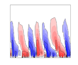
Some realisations of the mrOU process for different values of the parameter  $\theta \in [0,{\rm \pi} /2]$ are shown in figure 1. Note that $\theta =0$ corresponds to $A_t=1$ which recovers the deterministic HLP model, whereas $\theta ={\rm \pi} /2$ is a standard Ornstein–Uhlenbeck process with zero mean and unit variance. The family (2.8) is therefore highly suitable for the following numerical experiments, as it allows the QBO resulting from wave forcings with different intermittency properties to be compared, simply by changing the parameters $(\theta,\tau )$.

Figure 1. Realisations of wave amplitude  $A_t$ for different values of the parameter $\theta$ in the mrOU process (2.8) at equilibrium over a period 20 $\tau$. The labels LOW- $\theta$, MID- $\theta$, HIGH- $\theta$, MAX- $\lambda$ and MAX- $\theta$ correspond to $\theta =\{ {\rm \pi}/32,{\rm \pi} /7,{\rm \pi} /4,\sin ^{-1}(\sqrt {2/3}),{\rm \pi} /2 \}$, respectively.
3. Analysis of g-sHLP and the intermittency parameter
Our main results depend upon an asymptotic expansion using the non-dimensional time scale  $\tau$ of the stochastic process (2.5) as a small parameter. Recalling condition (C1), this means that the analysis is formally valid in the double limit
 \begin{equation} \varepsilon \ll \tau \ll 1. \end{equation}
Dimensionally, in the parent model, equation (3.1) requires the amplitude of the forcing waves to evolve on a time scale that is significantly longer than a typical wave period  $\sim \omega _*^{-1}$, but is significantly shorter than the streaming time scale $T_*$ which sets the QBO period. In the atmospheric situation, this corresponds to being longer than a few tens of minutes but shorter than $O(100\ {\rm days})$, which is plausible for the majority of non-orographic tropospheric wave sources, e.g. mesoscale convective systems.
Our main result applies to the g-sHLP (2.2) when the wave amplitudes  $A^\pm _t$ are driven by the general SDE (2.5). The detailed mathematical derivation is presented in Appendix A. The key idea is that when $\tau \ll 1$, the amplitudes $A^\pm _t$ in g-sHLP are ‘fast’ variables, and their leading-order effects on dynamics which takes place on longer time scales can be uncovered using the method of homogenisation. Our treatment of the problem is standard and closely follows the approach taken in Pavliotis & Stuart (Reference Pavliotis and Stuart2008, see Chap. 11), with the one additional complicating feature that, because g-sHLP is a stochastic integro-partial differential equation, as opposed to a regular SDE system, the backwards Kolmogorov equation (BKE) used in the derivation requires the use of functional calculus. However, this additional level of complexity does not change the essence of the derivation.
The main result of Appendix A is that the ‘slow dynamics’ of g-sHLP is governed by the following stochastic partial integro-differential equation, which describes the evolution of  $U(z,t)$ on the order unity time scale,
 \begin{align} {\rm d} U =\left( - \sum_{{\pm}} F_\pm[U,z] + \frac{1}{Re} \, \partial^2_z U +\lambda \sum_\pm \varPi_\pm[U,z] \right) {\rm d}t + \sqrt{2 \lambda} \left( \sum_\pm F_\pm[U,z] \, {\rm d}W^\pm_t \right). \end{align}
Equation (3.2), hereafter referred to as the homogenised equation, consists of the (generalised) deterministic HLP plus two correction terms due to the source intermittency, the first of which is deterministic and the second of which is stochastic, because the latter multiplies the increments of two independent Brownian processes  $W^\pm _t$. The functionals $\varPi _\pm$ appearing in the deterministic correction term depend only on $F_\pm$ and are given by
 \begin{equation} \varPi_\pm[V,z]= \int_{\mathcal{D}} F_\pm[V(\bar{z}),\bar{z}] \,\frac{\delta F_\pm}{\delta V(\bar{z})}[V(z),z] \, {\rm d}\bar{z}, \end{equation}
and can be evaluated for the specific example of sHLP, i.e. when  $F_\pm$ is given by (2.3), to be
 \begin{equation} \varPi_\pm[U,z] ={\pm} 2 F_\pm[U(z,t),z] \left( \int_0^z \frac{F_\pm[U(z',t)]}{({\pm} U(z',t)-1)^3}\, {\rm d}z' - \frac{F_\pm[U(z,t)]}{({\pm} U(z,t)-1)}\right). \end{equation}
Note that  $\varPi _{\pm }$ is derived from $F_\pm$, and consequently depends only on the deterministic part of the g-sHLP model. Crucially, it follows that there is just a single parameter $\lambda$ multiplying the correction terms in (3.2), the intermittency parameter
 \begin{equation} \lambda= \tau \int_{\mathbb{R}} a^2 q(a) p_s(a) \, {\rm d}a = \tau \mathbb{E}\left( A_t^2 q(A_t) \right), \end{equation}
where the function
 \begin{equation} q(a)= \int^a_{a_0} \frac{1}{g(x)^2 p_s(x)} \int_{-\infty}^x (1-y^2) p_s(y)\,{\rm d}y \,{\rm d}\kern0.06em x, \end{equation}
is obtained directly from the invariant density  $p_s(a)$ and noise function $g(a)$ of the process (2.5). The constant $a_0$ in (3.6) is chosen to satisfy $\int _{\mathbb {R}} q(a) p_s(a) \,{\rm d}a=0$. Since $F_\pm$ and $\varPi _\pm$ are properties of the deterministic part of the g-sHLP model, all of the stochastic behaviour associated with the SDE (2.5) is captured by the single parameter $\lambda$.
It is not necessary to solve the homogenised equation (3.2) to deduce the key prediction of our analysis:
(P) The corrections to the sHLP QBO due to source intermittency depend only on the value of the intermittency parameter
$\lambda$. This result applies to any process (2.5) satisfying conditions (C1)–(C3) for which $\lambda$ can be calculated.


There are several points to note about this result.
(i) It follows that, because intermittency induced changes to QBO properties such as the typical amplitude
$\mathcal {A}$ and period $\mathcal {P}$ depend only on $\lambda$, results for a wide range of different processes (2.5) with different time scales $\tau$ should collapse onto a single curve parameterised by $\lambda$.(ii) That
$\lambda$ depends linearly on the small parameter $\tau$ is a standard feature of homogenisation problems (see, e.g. Pavliotis & Stuart Reference Pavliotis and Stuart2008), and is a direct consequence of the asymptotic expansion. As $\tau$ is reduced so that the time scale of the intermittency becomes short, the QBO experiences only the averaged wave forcing from the boundary, demonstrating that deviations from the average forcing must be sustained in time in order to affect the QBO. As for all asymptotic theories, the theory will become inaccurate and then break down as $\tau$ increases, and the priority in the following is to determine when this occurs.(iii) The dependence of
$\lambda$ on the details of the forcing process (2.5), which emerges from the mathematics and is apparent in (3.5)–(3.6), is not easy to account for in full. It is clear from (3.5) that $\lambda$ is proportional to the second moment of the statistic $q(A_t)$ of the process $A_t$. What is less clear, however, is the interpretation of (3.6), i.e. what aspects of the SDE behaviour determines $q(a)$. Certainly $q(a)$ must take account of not only the distribution of forcing amplitudes, but also the typical residence times of the process at those amplitudes, in particular the extent to which large amplitude forcing is sustained by the process. Therefore, it is perhaps unsurprising that the noise function $g(a)$ appears in the denominator of the definition of $q(a)$, since low noise values are associated with longer residence times, and will lead to larger magnitudes for $q(a)$ and, thus, larger $\lambda$. However a complete understanding of the consequences of formulae (3.5) and (3.6), which determine which processes are more ‘intermittent’ than others, awaits further study.


It is straightforward to evaluate the intermittency parameter  $\lambda$ for the family of mrOU processes described in § 2.4. In this case $q(a)=a^2+2a \cos {\theta }-2\cos ^2{\theta }-1$ and it follows that
 \begin{equation} \lambda = \tau \sin^2{\theta}(4-3\sin^2{\theta}), \end{equation}
or, in terms of the standard deviation  $\sigma$ of the mrOU process, $\lambda = \tau \sigma ^2(4-3\sigma ^2)$. In figure 2, $\lambda /\tau$ is plotted against $\theta$. Interestingly, the ‘most intermittent’ member of the mrOU family (2.8) is not, as might be expected, the zero mean OU process ( $\theta ={\rm \pi} /2$, mean $\mu =0$, standard deviation $\sigma =1$) for which $\lambda /\tau =1$ but, in fact, occurs at $\theta =\sin ^{-1}(\sqrt {2/3})$ when $\lambda /\tau =4/3$. The reason appears to be that having a non-zero mean value allows the process to sustain larger amplitudes, despite it having smaller fluctuations. The implications of this result are tested in the next section.

Figure 2. Intermittency parameter  $\lambda$ scaled by $\tau$ for the sHLP model driven by the mrOU process (2.8) as a function of the mrOU parameter $\theta$.
4. Evaluation of the theory: numerical solutions of sHLP and the homogenised equation
The main objective in this section is to test the prediction (P), i.e. that the properties of the QBO in sHLP depend only on the value of the intermittency parameter  $\lambda$. An additional objective is to solve the homogenised equation (3.2) to test the following secondary prediction:
(P2) The QBO generated by the homogenised equation (3.2) matches those in sHLP at the same value of
$\lambda$.

A third objective is to test the limits of the theory and try to understand its breakdown, bearing in mind that it requires the time scale  $\tau \ll 1$ and will inevitably break down as $\tau$ approaches unity.
4.1. Evaluation of prediction (P): solutions of sHLP
The sHLP equation (2.2)–(2.3) with mrOU forcing (2.8) is solved using a numerical algorithm based on that described in Renaud et al. (Reference Renaud, Nadeau and Venaille2019). Although the numerical results here are for the mrOU family (2.8), it is important to emphasise that the theory predicts the same behaviour for any SDE (2.5) satisfying conditions (C2) and (C3). Some modifications have been made to the numerical algorithm, motivated primarily by the need to improve the convergence properties of the integrals terms in (2.3), particularly because accuracy is required when solving the homogenised model (3.2), as described in the following. A description of the modifications, along with other numerical details relating to integrating the mrOU equation, is given in Appendix B. All of the calculations to be described used a domain with height  $Z_d=3.5$, which is sufficiently high for the upper boundary to have negligible impact, and compared with Renaud et al. (Reference Renaud, Nadeau and Venaille2019) a high numerical resolution (grid spacing $\Delta z=10^{-3}$) is used. High resolution was found necessary to minimise the resolution-dependent behaviour reported in the supplementary material of Renaud et al. (Reference Renaud, Nadeau and Venaille2019).
Results from the simulations of sHLP at a typical Reynolds number ( ${Re}=10$) within the QBO generating regime are shown in figure 3. The upper left panel shows the QBO in the deterministic HLP (equivalently $\lambda =0$ in sHLP) which has a period $\mathcal {P}_0$ of 7.17 (units $T_*$). To obtain the amplitude of the deterministic QBO the standard deviation of $U(z,t)$ is calculated at every model level and the maximum value is taken, to give $\mathcal {A}_0\approx 0.70$ (units $U_*$). The same definition is used to calculate the amplitude $\mathcal {A}$ of the noisy QBOs generated by sHLP. To calculate the period $\mathcal {P}=2{\rm \pi} /\omega _p$ of the noisy QBOs in a consistent way a time series of $U(z_m,t)$, where $z_m$ is the level of the maximum root-mean-square $U$, is used. The time series has length $10^4 T_*$, equating to more than $10^3$ QBO periods, and data earlier than an initial spin-up period of 200 $T_*$ is discarded. The Fourier transform of this time series is then calculated, and the following weighted mean is used:
 \begin{equation} \omega_p=\left.\int_{\omega_-}^{\omega_+} \omega |\hat{F}(\omega)|^2 \, {\rm d}\omega \right/ \int_{\omega_-}^{\omega_+} | \hat{F}(\omega) |^2 \,{\rm d}\omega. \end{equation}
The low-pass and high-pass filters  $(\omega _-, \omega _+)=(0.2,2)$ are used to minimise spurious contributions due to the finite length of the time series at low frequencies and the mrOU process itself at high frequencies, and the remaining range captures the QBO spectral peak centred on $\omega \approx 1$.

Figure 3. Hovmöller diagram showing the mean wind  $U(z,t)$ in numerical solutions of the sHLP (2.2) between times $t=200$ and $t=230$. (a–c) The mrOU time scale $\tau = 10^{-2}$ and $\theta$ is varied: (a) deterministic HLP ( $\theta =0$); (b) $\theta ={\rm \pi} /8$; (c) $\theta ={\rm \pi} /5$. (d–f) The mrOU parameter $\theta ={\rm \pi} /2$ is fixed and: (d) $\tau =10^{-3}$; (e) $\tau = 10^{-2}$; and (f) $\tau = 10^{-1}$. In all cases ${Re}=10$. The corresponding values of $\lambda$ for (a–f) are $\lambda =\{0,5.21 \times 10^{-3},1.02\times 10^{-2},10^{-3},10^{-2},10^{-1} \}$.
The remaining left panels of figure 3 show the results for sHLP forced by the mrOU process with  $\tau =10^{-2}$ and $\theta ={\rm \pi} /8$ and $\theta ={\rm \pi} /5$ show progressively more noisy QBOs. In the right panels, $\theta ={\rm \pi} /2$ is fixed, and $\tau =\{10^{-3},10^{-2},10^{-1}\}$ is varied. Note that the principle of stochastic averaging is clearly demonstrated in figure 3(d), for which the intermittency parameter $\lambda =10^{-3}$ ( $\tau =10^{-3}, \theta ={\rm \pi} /2$) is very small, with the result that the sHLP QBO is almost indistinguishable from the deterministic HLP QBO shown in figure 3(a). As $\tau$ is increased the QBO variability increases, and the most noisy QBO in figure 3(f) exhibits arguably a similar level of random variability to observations (compare with, e.g. figure 1 of Newman et al. Reference Newman, Coy, Pawson and Lait2016).
A clear trend is evident in figure 3 towards longer periods as  $\lambda$ increases. Less immediately obvious is a trend towards lower QBO amplitudes. To assess these trends more fully the QBO amplitudes ( $\mathcal {A}/\mathcal {A}_0$) and periods ( $\mathcal {P}/\mathcal {P}_0$), measured relative to those of the deterministic HLP QBO $(\mathcal {A}_0,\mathcal {P}_0)$, are plotted in figure 4 for a wide range of sHLP simulations at different values of $\theta$ and $\tau$. The simulation details are given in table 1, and are grouped into sets in which one of the two parameters $(\theta,\tau )$ is held fixed and the other is varied to sweep out a large range of values of the intermittency parameter $\lambda$. The results clearly show that both the QBO amplitude $\mathcal {A}$ and period $\mathcal {P}$ collapse onto a single curve consistent with the prediction (P), provided that simulations with $\tau >0.1$ (filled symbols) are discounted. The reason for the apparent breakdown of the theory once $\tau \gtrsim 0.1$ is explored further in the following.

Figure 4. QBO amplitudes  $\mathcal {A}^*=\mathcal {A}/\mathcal {A}_0$ and periods $\mathcal {P}^*=\mathcal {P}/\mathcal {P}_0$ from the respective families of sHLP simulations detailed in table 1, as a function of the intermittency parameter $\lambda$. Results from the simulations of higher-order modes of the homogenised equation (3.2) (red pentagram) are also shown in the inset. Results are scaled by the deterministic HLP amplitude $\mathcal {A}_0=0.7$ and period $\mathcal {P}_0=7.17$. Filled symbols correspond to simulations with $\tau >0.1$.
Table 1. The sets of sHLP simulations at different values of the mrOU parameters  $(\theta,\tau )$ used to generate the data in figure 4. In the experiment set FIX- $\tau$, $\tau$ is fixed and $\theta$ is varied, whereas in the remaining experiment sets $\theta$ is fixed and $\tau$ is varied. Each experiment set corresponds to the given values of the intermittency parameter $\lambda$.

4.2. Evaluation of prediction (P2): solutions of the homogenised equation
Solving the homogenised equation (3.2) directly is an appealing alternative to the sHLP for calculating the QBO properties for different values of  $\lambda$. However, the numerical solution of (3.2) has proved challenging. The main reason is that, given a typical wind profile $U(z,t)$, the functionals $\varPi _\pm [U,z]$ appearing in (3.2) generally feature a rapidly changing thin boundary layer in the vicinity of the maxima of the jets (see the following). Moreover, the details of this boundary layer are highly sensitive to small changes in $U$ close to the maxima, meaning that high temporal and spatial resolution is required to accurately resolve $\varPi _\pm$ as $U$ evolves. Using the improved algorithm described in Appendix B to evaluate the integrals required to calculate $\varPi _\pm$, the numerical cost of solving (3.2) at larger values of $\lambda$ exceeds that of sHLP by two orders of magnitude, with the cost increasing as $\lambda$ is increased. In the absence of a more bespoke algorithm for (3.2), numerical solutions at only the lowest values of $\lambda =\{ 10^{-4}, 5 \times 10^{-4} \}$ have been found to be computationally tractable.
The QBO amplitude  $\mathcal {A}$ and period $\mathcal {P}$ calculated from the solutions to (3.2) have been plotted in figure 4 (cyan triangles; see the insets in particular). The results are consistent with the sHLP calculations, at least within the statistical error of our calculations, showing that the homogenised equation (3.2) does indeed reproduce the behaviour of the sHLP as predicted. More broadly, however, it is a disappointing outcome of our analysis that the equation (3.2) is difficult to use in practice, although it remains possible that an improved numerical algorithm could rectify this problem.
4.3. Assessment of the breakdown of the theory as $\tau$ increases

Analysis of the terms in the homogenised equation (3.2) allows some insight into why the theory appears to break down at relatively low values of the mrOU time scale  $\tau$. In figure 4 results from simulations with $\tau \gtrsim 0.1$ (solid points) deviate significantly from the curves traced out by the remaining sHLP solutions. Physically, in the atmospheric situation, if the streaming time scale $T_*$ is taken to be 100 days this corresponds to around 10 days, which is greater than the time scale generally associated with gravity wave packets in the upper troposphere.
Figure 5 plots the height profile of  $F_+[U,z]$ and $\varPi _+[U,z]$ for the sHLP (given by (2.3) and (3.4), respectively) for a representative flow profile $U(z)$ shown in the left panel. These plots give some insight into why the theory breaks down at what might appear to be a comparatively low value of $\tau$. The key point is the large factor (approximately 150) between the absolute value of the magnitude of $\varPi _+[U,z]$ compared with that of $F_+[U,z]$. Formally, because $\tau \ll 1$ in the asymptotic theory, the contribution from the deterministic correction $\lambda \varPi _+[U,z]$ is infinitesimal compared with that from $F_+[U,z]$. However, in practice, at finite $\tau$, the correction term $\lambda \varPi _+[U,z]$ becomes comparable in magnitude to $F_+[U,z]$ at relatively low values of $\tau$, thus bringing the predictions of the theory into question.

Figure 5. (a) Analytic solution (B5) of Renaud et al. (Reference Renaud, Nadeau and Venaille2019) and (b) computation of  $F_+$ (B6) and (c) $\varPi _+$ (B7) for $Re=10$.
5. Discussion and conclusions
5.1. Extension to broadband forcing
The HLP model is, by design, an idealised system with the aim of demonstrating QBO-like behaviour in as simple a setting as possible. It is clear, however, that since our main results were obtained in the generalised setting of g-sHLP they apply equally to more sophisticated gravity wave parameterisation schemes, since changing the nature of the waves and the details of the wave dissipation will result in only changes to  $F_\pm$, and our main results apply to any $F_\pm$.
The remaining key simplification of our study is, however, the restriction to near-monochromatic wave forcing in the wave source (2.4), and that this forcing is confined to the lower boundary. The forcing in sHLP is best described as ‘near-monochromatic’ here, because, due to the formal time scale separation between the fast evolution of the waves, which evolve on an  $O(\varepsilon )$ time scale and the forcing Ornstein–Uhlenbeck process, which evolves on a time scale $O(\tau )$ the spectral broadening due to the time dependence of the stochastic forcing in sHLP is infinitesimal. It is important to note that this would not be the case in the parent Boussinesq model in which both $\varepsilon$ and $\tau$ are finite. In reality, the QBO is forced by a spectrum of different types of waves due to many physical processes, some of which (e.g. convective forcing; see Lecoanet et al. Reference Lecoanet, Le Bars, Burns, Vasil, Brown, Quataert and Oishi2015) are best represented as a bulk forcing which is distributed in the vertical rather than as a localised boundary forcing. Our view is that a clear next step in building towards greater realism is to consider HLP with a broad source spectrum (e.g. $\mathcal {K}(k,\omega )$ for kinetic energy) in wavenumber–frequency space. It is known (e.g. Léard, Lecoanet & Le Bars Reference Léard, Lecoanet and Le Bars2020) that broadening the source spectrum does not change the essential nature of the QBO, except to make the periodic signal more robust, and tends to lead to longer QBO periods and increased amplitudes. Extending the current work to the most general broadband forcing situation is a significant undertaking, not least because the class of available random processes [e.g. stochastic partial differential equations (SPDEs)] which could drive a randomly evolving bottom boundary $h(x,t)$ is very large. Some questions which arise naturally are as follows.
A. If a class of SPDEs is specified to drive a randomly evolving broadband forcing
$h(x,t)$, can results analogous to the intermittency parameter be obtained?B. In the broadband case, does the intermittency parameter
$\lambda$ determining the QBO in the monochromatic case generalise to an intermittency spectrum $\varLambda (k,\omega )$? This seems a reasonable hypothesis, and it seems necessary to have to consider the spectral dependence of the intermittency, given that observed sources of different types are likely to have different intermittency properties.C. Assuming B, can stochastic parameterisations, of the type introduced by Eckermann (Reference Eckermann2011), Lott et al. (Reference Lott, Guez and Maury2012) and Lott & Guez (Reference Lott and Guez2013) be developed to match not only the source spectrum
$\mathcal {K}(k,\omega )$ but also the intermittency spectrum $\varLambda (k,\omega )$? In addition to being computationally efficient, such parameterisations would have the potential allow GCMs to capture the QBO response to changes in the nature of the wave forcing which go beyond changes to the launch spectrum.D. Again assuming B, given a randomly evolving lower boundary
$h(x,t)$, driven by an unknown process, what basic statistics of $h$ can be used to estimate $\varLambda (k,\omega )$? This question is crucial because it is clearly a difficult and underconstrained problem to choose an SPDE model for the wave forcing in practice.


5.2. Summary and outlook
Here a random component has been added to the wave forcing in the HLP model of the QBO in order to assess the impact of an intermittent wave source. Remarkably, it was found that the impact on the QBO when the forcing wave amplitude is controlled by any of a wide class of stochastic processes (2.5), can be captured by a single intermittency parameter  $\lambda$ given by (3.5). The result exploits the fact that the QBO time scale is much longer than the time scale on which the source amplitudes will vary, a time scale separation which will hold for most wave sources in the tropical atmosphere, arguably with the partial exception of longer lived intraseasonal variability, such as the Madden–Julian oscillation.
The results raise the prospect of designing new stochastic parameterisations for unresolved gravity waves in GCMs which rely less on artificial tuning parameters (e.g. the efficiency factor in the scheme of Alexander & Dunkerton Reference Alexander and Dunkerton1999), and display a generally greater fidelity to the physics. In a climate model, such a scheme could better capture the response of the circulation to changes in wave forcing which go beyond changes to the source kinetic energy spectrum. A possible programme to develop such a scheme could be based on answering questions A–D above, although care will be necessary in ensuring that each member of the hierarchy of models (i.e. HLP to parent Boussinesq model to GCM) remains qualitatively relevant and captures the essential physical processes taking place.
Funding
This work was supported by the Natural Environment Research Council (grant number NE/S00985X/1).
Declaration of interests
The authors report no conflict of interest.
Appendix A. Derivation of the homogenised equation (3.2)
Here the homogenised equation (3.2) is derived from the g-sHLP (2.2) when the fast variables  $A^\pm _t$ are driven by an SDE process (2.5) satisfying conditions (C1)–(C3), in addition to the scaling (3.1) which is necessary in order that $\tau$ can be treated as a small parameter. The derivation follows the approach taken in chapter 11 of Pavliotis & Stuart (Reference Pavliotis and Stuart2008).
First, consider the following conditional expectation, which is evaluated from the solution  $U(z,t)$ of the g-sHLP (2.2) at a fixed constant final time $t$
$t$
 \begin{equation} \varGamma[ V, a_+, a_-, s]= \mathbb{E} \left( \varPhi[ U(z,t), A_t^+, A_t^- ] \ | \ U(z,s)=V(z), A_s^\pm=a_\pm \right). \end{equation}
Here  $\varGamma$ and $\varPhi$ are scalar functionals. The functional $\varGamma$ has dependencies based upon the initial conditions for the g-sHLP, e.g. $U(z,s)=V(z)$ which are applied at a time $s< t$, as well as corresponding initial conditions $a_\pm$ for the respective wave amplitudes. It is not necessary for the following to specify a particular form for $\varPhi$. As detailed in Pavliotis & Stuart (Reference Pavliotis and Stuart2008), it is known that expressions of the type $\varGamma$ satisfy the BKE, which for g-sHLP is
 \begin{equation} \partial_s \varGamma + \frac{1}{\tau} \sum_\pm \mathcal{L}_0^\pm \varGamma + \mathcal{L}_1 \varGamma =0, \end{equation}
where the linear operators  $\mathcal {L}_0^\pm$ and $\mathcal {L}_1$ are defined according to
 \begin{align} \mathcal{L}_0^\pm \varGamma & \equiv f(a_\pm) \partial_{a_\pm} \varGamma + g(a_\pm)^2 \partial^2_{a_\pm} \varGamma \end{align}
 \begin{align} \mbox{and} \quad \mathcal{L}_1 \varGamma & \equiv \int_{\mathcal{D}} Q_V[V(z),z,a_+,a_-] \, \frac{\delta \varGamma}{\delta V(z)} \,{\rm d}z \end{align}
 \begin{align} & \equiv \lim_{\varepsilon \to 0} \frac{\rm d}{{\rm d}\varepsilon} \left( \varGamma[ V(z)+\varepsilon Q_V[V(z),z,a_+,a_-], a_+, a_-, s] \right) \end{align}
 \begin{align} \mbox{where}\quad Q_V[V,z,a_+,a_-] & =- \sum_{{\pm}} (a_\pm)^2 F_\pm[V,z] + \frac{1}{Re} \, \partial^2_z\, V, \end{align}
and where  $F_\pm$ are the functionals defined in (2.2).
The homogenised equation is obtained by seeking a solution to the BKE in the form of an asymptotic expansion in the small parameter  $\tau$,
 \begin{equation} \varGamma = \varGamma_0 + \tau \varGamma_1 + \tau^2 \varGamma_2 +\cdots . \end{equation}
At leading order in  $\tau$
 \begin{equation} \mathcal{L}_0^\pm \varGamma_0 =0, \end{equation}
from which we conclude that  $\varGamma _0$ is independent of $a_\pm$, i.e.
 \begin{equation} \varGamma_0 = \bar{\varGamma}_0[V(z),s]. \end{equation}
This conclusion is justified by the fact that the relevant null space of  $\mathcal {L}_0^\pm$ is spanned by the identity function, which is a property of all SDEs satisfying the ergodic property (C2) (see, e.g. chapter 6 of Pavliotis & Stuart Reference Pavliotis and Stuart2008).
At next order,
 \begin{equation} \sum_\pm \mathcal{L}_0^\pm \varGamma_1 =- \partial_s \bar{\varGamma}_0 - \mathcal{L}_1 \bar{\varGamma}_0. \end{equation}
First, this equation has a solvability condition
 \begin{equation} \int_{\mathbb{R}} \int_{\mathbb{R}} \left( \partial_s \bar{\varGamma}_0 + \mathcal{L}_1 \bar{\varGamma}_0 \right) p_s(a_+) p_s(a_-) \, {\rm d}a_+ \,{\rm d}a_-=0. \end{equation}
This result follows because the invariant density  $p_s(a)$ spans the null space of $\mathcal {L}_0^*$, the adjoint of $\mathcal {L}_0$. Since $\mathbb {E}((A^\pm _t)^2)=1$ the integrals in the solvability condition can be evaluated to give
 \begin{equation} \left.\begin{gathered} \partial_s \bar{\varGamma}_0 + \int_{\mathcal{D}} Q^0_V[V,z] \, \frac{\delta \bar{\varGamma}_0}{\delta V} \, {\rm d}z =0, \quad \mbox{where} \\ Q^0_V[V,z] =- \sum_\pm F_\pm[V,z] + \frac{1}{Re} \, \partial^2_z V. \end{gathered}\right\}\end{equation}
This equation for  $\bar {\varGamma }_0$ can be interpreted as the (deterministic) BKE associated with the standard HLP model ( $A_t^\pm =1$ in the sHLP above). To find more interesting behaviour, we need to go to the next order, which requires the full solution for $\varGamma _1$, which is obtained from
 \begin{align} \sum_\pm \mathcal{L}_0^\pm \varGamma_1 & = \int_{\mathcal{D}} \left( Q^0_V[V,z] -Q_V[V,z,a_+,a_-] \right) \frac{\delta \bar{\varGamma}_0}{\delta V} \, {\rm d}z \nonumber\\ & =- \sum_\pm (1-a_\pm^2) \int_{\mathcal{D}} F_\pm[V,z] \, \frac{\delta \bar{\varGamma}_0}{\delta V} \, {\rm d}z. \end{align}
To solve this system we need a particular integral  $q(a)$ for the ordinary differential equation
 \begin{equation} f(a) q'(a) + g(a)^2 q''(a) = 1-a^2, \end{equation}
which is
 \begin{equation} q(a)= \int_{a_0}^a \frac{h(x)}{g(x)^2 p_s(x)} \,{\rm d}\kern0.06em x, \quad \mbox{where} \ h(a)=\int_{-\infty}^a (1-x^2)p_s(x) \, {\rm d}\kern0.06em x. \end{equation}
The lower limit  $a_0$ in the integral is chosen for convenience (without loss of generality as it can be shown not to affect the value of the constant $\gamma$ defined in the following), to satisfy $\mathbb {E}(q(A^\pm _t))=\int _{\mathbb {R}} q(a) p_s(a) \, \textrm {d}a=0$. The solution is then
 \begin{equation} \varGamma_1=\bar{\varGamma}_1[V] - \sum_\pm q(a_\pm) \int_{\mathcal{D}} F_\pm[V,z] \, \frac{\delta \bar{\varGamma}_0}{\delta V} \, {\rm d}z. \end{equation}
To find the slow dynamics equation, the next order equation must be considered
 \begin{equation} \sum_\pm \mathcal{L}_0^\pm \varGamma_2 =- \partial_s \varGamma_1 - \mathcal{L}_1 \varGamma_1. \end{equation}
The solvability condition for (A17) is
 \begin{equation} \int_{\mathbb{R}} \int_{\mathbb{R}} \left( \partial_s \varGamma_1 + \mathcal{L}_1 \varGamma_1 \right) p_s(a_+) p_s(a_-) \, {\rm d}a_+ \,{\rm d}a_-=0, \end{equation}
which can be evaluated to be
 \begin{align} &\partial_s \bar{\varGamma}_1 + \int_{\mathcal{D}} Q^0_V[V,z] \, \frac{\delta \bar{\varGamma}_1}{\delta V} \, {\rm d}z +\gamma \sum_\pm \int_{\mathcal{D}} \int_{\mathcal{D}} F_\pm[V(\bar{z}),\bar{z}] \frac{\delta F_\pm}{\delta V(\bar{z})} \, \frac{\delta \bar{\varGamma}_0}{\delta V(z)} \, {\rm d}z \, {\rm d}\bar{z}\nonumber\\ &\quad + \gamma \sum_\pm \int_{\mathcal{D}} \int_{\mathcal{D}} F_\pm[V(z)] F_\pm[V(\bar{z})] \, \frac{\delta^2 \bar{\varGamma}_0}{\delta V(z)\delta V(\bar{z})} \, {\rm d}z \, {\rm d}\bar{z}=0, \end{align}
where
 \begin{equation} \gamma = \int_{\mathbb{R}} a^2 q(a) p_s(a) \, {\rm d}a = \mathbb{E}\left( A_t^2 q(A_t)\right). \end{equation}
Combining (A12) $\,+\,\tau $(A19) gives the following equation for $\bar {\varGamma }=\bar {\varGamma }_0+\tau \bar {\varGamma }_1$, correct up to $O(\tau )$:
 \begin{align} &\partial_s \bar{\varGamma} + \int_{\mathcal{D}} Q^0_V[V(z)] \, \frac{\delta \bar{\varGamma}}{\delta V} \,{\rm d}z +\tau \gamma \sum_\pm \int_{\mathcal{D}} \int_{\mathcal{D}} F_\pm[V(\bar{z}),\bar{z}] \, \frac{\delta F_\pm}{\delta V(\bar{z})} \, \frac{\delta \bar{\varGamma}}{\delta V(z)} \,{\rm d}z \, {\rm d}\bar{z} \nonumber\\ &\quad + \tau \gamma \sum_\pm \int_{\mathcal{D}} \int_{\mathcal{D}} F_\pm[V(z),z] F_\pm[V(\bar{z}),\bar{z}] \, \frac{\delta^2 \bar{\varGamma}}{\delta V(z) \delta V(\bar{z})} \, {\rm d}z \, {\rm d}\bar{z}=0. \end{align}
This equation for  $\bar {\varGamma }$ can be recognised as the BKE corresponding to the following ‘slow dynamics’ equation:
 \begin{align} {\rm d} U &=\left( Q^0_V[U,z] + \tau \gamma \sum_\pm \int_{\mathcal{D}} F_\pm[U(\bar{z},t),\bar{z}] \,\frac{\delta F_\pm}{\delta V(\bar{z})}[U(z,t),z] \, {\rm d}\bar{z} \right) {\rm d}t \nonumber\\ &\quad + \sqrt{2 \gamma \tau} \left( \sum_\pm F_\pm[U(z,t),z] \, {\rm d}W^\pm_t \right), \end{align}
where  $W^\pm _t$ are two independent Brownian processes. Substituting for $Q^0_V$ recovers the homogenised model (3.2) on defining the intermittency parameter to be $\lambda =\gamma \tau$.
Appendix B. Details of the numerical algorithms for (2.2) and (3.2)
The algorithm used to solve sHLP is adapted from the finite-difference scheme described in the supplemental material of Renaud et al. (Reference Renaud, Nadeau and Venaille2019). The most significant alteration is an improved scheme for evaluating the integrals
 \begin{equation} I_{{\pm}}(z)=\int_0^{z} \frac{1}{({\pm} U(z')-1)^2}\,{\rm d}z', \end{equation}
which appear in the exponential terms in (2.2). The reason an improved scheme is necessary is that to obtain accurate solutions of (3.2) it is essential that the behaviour of the calculated  $I_\pm (z_i)$ at a grid point $z=z_i$ varies smoothly as the relative position of a nearby critical line at $z=z_c$, defined to be where $\pm U(z_c)-1=0$, is varied. Following Renaud et al. (Reference Renaud, Nadeau and Venaille2019), the value of $I_\pm$ is set to $+\infty$ for all grid points above $z=z_c$, corresponding to setting to zero the exponential in (2.2). However, if $I_\pm$ is evaluated using a grid-based quadrature as in Renaud et al. (Reference Renaud, Nadeau and Venaille2019), then $I_\pm (z_i)$ exhibits considerable grid-based sensitivity to the relative position of $z_c$ and the grid points immediately below $z_{i}$.
To alleviate the above issue,  $I_\pm$ is evaluated in our scheme for the piecewise linear interpolant of $U(z)$, i.e.
 \begin{equation} U_P(z)=U(z_i)+ \left( U(z_{i+1})- U(z_i) \right) \frac{z-z_i}{\varDelta z}, \quad\text{for} \ z \in [z_i,z_{i+1}]. \end{equation}
The advantage of this approach is that  $I_\pm$ can be evaluated exactly for $U_P$ as
 \begin{equation} I_\pm(z_i)=\sum_{j \leqslant i} \frac{\Delta z}{({\pm} U(z_j)-1)({\pm} U(z_{j-1})-1)} \end{equation}
and (B3) gives smoother behaviour compared with more basic quadratures. Higher-order approximations based on cubic interpolation or splines naturally suggest themselves as further improvements, although these are not necessary for a robust scheme.
To assess the appropriate choice of the appropriate grid size  $\Delta z$, the absolute errors $E_{F}$ and $E_\varPi$ of $F_+$ and $\varPi _+$, measured in the L $_2$ norm, are calculated for the exact test case profile of Renaud & Venaille (Reference Renaud and Venaille2020), which is the steady solution of the following ‘single-wave’ version of HLP:
 \begin{equation} \frac{1}{{Re}} \partial^2_{z}U =\partial_z\left(\exp\left(-\int_0^z\frac{1}{(U(z')-1)^2}\, {\rm d}z'\right)\right). \end{equation}
The exact solution is written in terms of the Lambert- $W$ function $W({\cdot })$, as
 \begin{equation} U(z) =\frac{{Re}-L(z)}{1+{Re}},\quad \mbox{where}\ L(z)=W\left({Re} \exp\left({Re}-z\left({Re}+1\right)^2\right)\right), \end{equation}
and the errors  $E_F$ and $E_\varPi$ can be calculated using the analytical results
 $$\begin{gather} F_+(z)=\frac{L(z)}{{Re}}\left(\frac{{Re}+1}{L(z)+1}\right)^3, \end{gather}$$
 $$\begin{gather}\varPi_+(z) = \frac{1}{2 {Re}^2}\left(\frac{{Re}+1}{L(z)+1}\right)^7L(z)\left[\left(\frac{L(z)+1}{{Re}+1}\right)^4+4L(z) -1\right]. \end{gather}$$
Figure 6 shows  $E_F$ and $E_\varPi$ as a function of grid size $\Delta z$. Quadratic convergence is evident for $F_+$ and linear convergence for $\varPi _+$. This can be verified by comparison with analytic expressions for $F$ and $\varPi$ which are independent of grid size, obtained by using (B5).

Figure 6. Errors  $E_F$ and $E_\varPi$ in the ${L}_2$-norm of $F_+$ (2.3) and $\varPi _+$ (3.4) for the analytic solution (B5) of Renaud et al. (Reference Renaud, Nadeau and Venaille2019). In each case $Re=10$.
Timestepping of the mrOU process follows the algorithm of Gillespie (Reference Gillespie1996) with timestep  $\Delta t =10^{-4}$, chosen so that $\Delta t/\tau$ is small in all circumstances, in order to resolve the process adequately. For timestepping of (2.2) for stability the implicit backward difference scheme is used. This scheme is unconditionally stable and avoids spurious oscillations.


 Open access