


1. Introduction
The subaqueous pendulum is a core model in fluid dynamics of important interest in research but also for educational purposes, that is, to introduce students to the basic concepts of dynamics and harmonic motions (Mongelli & Battista Reference Mongelli and Battista2020). Stokes (Reference Stokes1851) demonstrated the pendulum's usefulness to study drag force. About 170 years after Stokes (Reference Stokes1851), experimental research on spherical (Dolfo, Vigué & Lhuillier Reference Dolfo, Vigué and Lhuillier2020) and cylindrical (Dolfo, Vigué & Lhuillier Reference Dolfo, Vigué and Lhuillier2021) pendulums, in the limit of small Reynolds numbers  $\textit {Re}<1$, was conducted. For small oscillation amplitudes, the corresponding Stokes numbers were in the range $St\in [153, 1500]$ in Dolfo et al. (Reference Dolfo, Vigué and Lhuillier2020) and $St\in [0.2, 230]$ in Dolfo et al. (Reference Dolfo, Vigué and Lhuillier2021).
Govardhan & Williamson (Reference Govardhan and Williamson1997) measured the motion of a pendulum-like tethered sphere in a uniform flow and attempted to gain insight into vortex-induced vibrations (VIVs). Williamson & Govardhan (Reference Williamson and Govardhan1997) illustrated that different modes of amplitude and frequency responses could result in nearly doubling the drag force of the oscillating sphere when compared with a stationary one. Obligado, Puy & Bourgoin (Reference Obligado, Puy and Bourgoin2013) investigated the stability of a pendular disk facing an incoming flow. They reported significant stability changes related to turbulent drag enhancement.
More recently, Mathai et al. (Reference Mathai, Loeffen, Chan and Wildeman2019) studied the dynamics of heavy and buoyant subaqueous pendulums with cylindrical bobs and large amplitudes, using different mass ratios  $m^*=\rho _s/\rho _F$, where $\rho _s$ and $\rho _F$ are the density of pendulum and fluid, respectively. They derived a mathematical model equation of motion and they further improved it by including the wake flow caused by the back-swing of cylinders through the disturbed flow field. Mathai et al. (Reference Mathai, Loeffen, Chan and Wildeman2019) conducted a series of two-dimensional particle image velocimetry (2D-PIV) experiments to analyse the flow field and to visualise the shedding of vortices during the downward swing. They found that due to the finite length of the cylinder, the added mass coefficient is significantly lower than the potential flow value of $m_a = 1$.
Worf et al. (Reference Worf, Khosronejad, Gold, Reiterer, Habersack and Sindelar2022) numerically re-investigated the subaqueous cylinder pendulum of Mathai et al. (Reference Mathai, Loeffen, Chan and Wildeman2019), using large-eddy simulations (LES). Their findings suggest that the deviation in the added mass is caused by the predominance of a three-dimensional (3-D) flow field featuring tip vortices during the first downward swing. Wake interactions occur already before the cylinder swings back. Therefore, Worf et al. (Reference Worf, Khosronejad, Gold, Reiterer, Habersack and Sindelar2022) suggest starting the wake correction proposed by Mathai et al. (Reference Mathai, Loeffen, Chan and Wildeman2019) already before the first turning point. Hence, even with the cylinder, which could be interpreted as a two-dimensional (2-D) flow, only the 3-D analysis adequately explains all the predominant flow phenomena. Mongelli & Battista (Reference Mongelli and Battista2020) performed numerical fluid–structure interaction (FSI) simulations of pendulums with a spherical bob and different radii. In their 2-D simulations, they considered a short slice of a cylinder to represent the sphere. Regarding the vortex shedding topology of subaqueous pendulums with 3-D spherical bobs, Bolster, Hershberger & Donnelly (Reference Bolster, Hershberger and Donnelly2010) suggested that for large amplitudes, vortex streets are induced by the shedding of vortices at the turning points that, in turn, lead to additional drag forces over the spherical bob.
Raffel et al. (Reference Raffel, Willert, Scarano, Kähler, Wereley and Kompenhans2018) and Schröder & Schanz (Reference Schröder and Schanz2023) reported the recent advances in laser-optical flow measurement techniques that allow for more rigorous investigation of vortex–structure interactions. For instance, Gold et al. (Reference Gold, Reiterer, Worf, Khosronejad, Habersack and Sindelar2023) used time-resolved 3-D particle tracking velocimetry (tr-3D-PTV) and a digital object tracking (DOT) method to obtain a characteristic vortex shedding topology during the first downward pendulum swing of oscillating spheres of various mass ratios  $m^*\in [1.14,14.95]$. They observed that, first, a toroidal vortex is formed in the sphere's wake, which then splits up into two separate vertical structures of equal size (Gold et al. Reference Gold, Reiterer, Worf, Khosronejad, Habersack and Sindelar2023). They also showed that the time when the first vortex is shed, and its initial propagation velocity, depend on $m^*$ (Gold et al. Reference Gold, Reiterer, Worf, Khosronejad, Habersack and Sindelar2023). In essence, the DOT method combines the temporal and spatial information gained from tr-3D-PTV recordings by treating vortex representations as distinct digital objects to analyse vortex dynamics (Gold et al. Reference Gold, Reiterer, Worf, Khosronejad, Habersack and Sindelar2023). Further, Gold et al. (Reference Gold, Reiterer, Worf, Khosronejad, Habersack and Sindelar2023) suggests a wake correction model for heavy spherical pendulums underwater that already starts with the shedding of the first vortex. Importantly, Young et al. (Reference Young, Li, Capart and Chu2022) stressed the important role of the pressure dynamics in the particle–vortex interaction of (freely) falling spheres in a fluid. Lastly, it should be noted that the existing Lagrangian particle tracking methods are capable of obtaining the flow field pressure using the Navier–Stokes equations (van Oudheusden Reference van Oudheusden2013; Raffel et al. Reference Raffel, Willert, Scarano, Kähler, Wereley and Kompenhans2018).
This study aims at (i) extending our current understanding of the subaqueous pendulum dynamics for large amplitudes and (ii) developing an improved model equation of motion for the subaqueous pendulum for a wide range of solid-to-fluid mass ratios. To do so, we carried out a series of experiments with heavy pendulums of spherical bobs, for eight different solid-to-fluid mass ratios  $m^*\in [1.14, 14.95]$, and for a range of Reynolds number in the order of $\textit {Re}\sim O(10^4)$. In these experiments, we improved the tr-3D-PTV measurement system of Gold et al. (Reference Gold, Reiterer, Worf, Khosronejad, Habersack and Sindelar2023) to analyse the 3-D flow and pressure fields around the subaqueous pendulum. Furthermore, we seek to improve the model equation of motion for the subaqueous pendulum, which was previously reported in Mathai et al. (Reference Mathai, Loeffen, Chan and Wildeman2019), by examining the high-speed single-frame (SF) recordings of the pendulum. The basic model equation underestimates the peak amplitude for all $m^*$ and is incapable of accurately obtaining the period for the pendulum solid-to-fluid mass ratios of $m^*<2$. Importantly, we show that considering both the vortex-induced drag (VID) and a history force term, related to 3-D wake interactions, allows for a significant improvement of the predictions of the model equation. Finally, our findings regarding the initiation of the wake model application show that the most accurate model fit is achieved by using the temporal information of first vortex shedding.
This paper is organised as follows. In § 2, we describe the experimental methods used in this study. Subsequently, in § 3, the proposed model equation of motion of subaqueous pendulums is presented, and its limitations to describe the dynamics of motion are discussed. Finally, the findings of the study and future research perspectives are summarised in § 4.
2. Experiments
2.1. Experimental system
The carrying system for the experimental set-up and measuring equipment is a table-like construction made of aluminium rail profiles, grounded on damped leveling feet. The experiments are performed in a 600-mm-long, 300-mm-wide and 300-mm-high glass tank, placed over the volume optic (VO). In figure 1, we depict details of the experimental set-up. As can be seen, several aluminium rails with glass clamps attach the pendulum and its release device to the glass tank. The release device is an adaptive mechanical gripper (NIRYO Robotics) over a guiding arm. A microcontroller (OpenCM9.04, Type C) operates small movements of the gripper to avoid disturbing the flow field. A nylon string with a diameter of 0.05 mm, attached to a ball bearing, is used as the pendulum thread. Spheres of different materials with the same diameter  $D$ of 12.71 mm, representing the pendulum bob, are glued to the loose end of the string. Table 1 lists the materials and their specific properties in the experiments. To avoid undesirable illumination peaks, and to reduce the friction differences caused by their surface roughness, all spheres were painted black.

Figure 1. Schematics of the experimental set-up for the single frame recording (SF) and 3D-PTV measurements. (a) Side view. (b) Plan view: SF set-up that is highlighted in red (CAM II), 3D-PTV system is marked with the green rectangle (CAM I-CAM IV), VC is the video camera. (c) 3-D sketch of the tank set-up with the camera alignment and the sphere that is coloured in yellow.
Table 1. Material properties of the pendulum spheres with a diameter of  $D = 12.71$ mm.

Initially, the sphere is 2.2 $D$ below the water level, while at its lowest position, it is located 8.5 $D$ above the base of the tank. The distance to the sidewalls is ${>}10D$. The pendulum length of $L =200$ mm is measured from the bearing to the centre of the sphere and the initial angular deflection is $\theta =37.5^\circ$. A self-designed adjustment tool is used to guarantee the same initial position throughout the experiments (Gold et al. Reference Gold, Reiterer, Worf, Khosronejad, Habersack and Sindelar2023) with pendulums of various solid-to-fluid mass ratios.
After a 3-minute waiting interval to damp out disturbances in the fluid, the buffer-recording mode is started. When the gripper releases the sphere, the trigger initiates the saving of the past 200 images and the recording of further 3800 images. A high-speed PTV system from LaVision is used. This system includes four high-speed cameras (Imager Pro HS 4M CMOS) and a high-speed laser (ND:YLF-PIV Laser,  $E = 30$ mJ, $\lambda = 527$ nm) of the Litron LDY series. The cameras (CAM I–IV) have a resolution of $2016 \times 2016$ pixels. Each camera is equipped with a Scheimpflug adapter (SP in figure 1b) which is empirically adjusted during the calibration procedure. The approximate Scheimpflug angles are $2^\circ$ for CAM I, $0^\circ$ for CAM II, $2^\circ$ for CAM III and $3^\circ$ for CAM IV. In addition, a video camera ( ${\rm VC} = {\rm iPhone}$ 12, HD 1080p, $1920\times 1080$ pixels), orthogonal to the $Y\unicode{x2013}Z$ plane and operating at 240 frames per second, is used to determine the maximum $Z$-displacement of the sphere. From VC we manually extracted the maximum ratio between the $Z$-displacement in pixel and the spheres diameter in pixel of the same image frame. The length scale of VC ranged from 7 to $11\ {\rm pixel}\ {\rm mm}^{-1}$. The laser head emits a laser beam with a diameter of 5 mm and is connected to a VO via an optical guiding arm. The two-component VO expands the laser beam to the desired volume. Further, three mirrors (MIR) reflect the laser light to regions with shadows cast by the sphere. A mechanical aperture (MA) is placed above the VO to suppress unsharp edges. The timing synchronisation is managed using a programmable timing unit (PTU; PTUX by LaVision) operated by the Davis 10.1 by LaVision software. The trigger is a photoelectric barrier (Sick WL8) that is connected to the trigger input of the PTU. The system consists of a reflector (REF) and a photoelectric sensor (S/E) to transmit and receive the light signal, both mounted on two guiding rails. In its initial position, the sphere pendulums interrupt the signal of the photoelectric barrier. A LED (Veritas Constellation 120) is used to illuminate the tank during the camera adjustment, calibration and single-frame recordings (CAM II) without the laser. Lastly, to calibrate the camera, we employed a 3-D calibration plate (204-15 by LaVision, $204\times 204$ mm) with two different planes (level separation of 3 mm) and dot-shaped markers (spacing of 15 mm).
2.1.1. Particle tracking velocimetry
To perform the tr-3D-PTV measurements, the water was seeded using the polyamide tracer particles with a mean diameter of  $50\ \mathrm {\mu }{\rm m}$ and a density of $1.016\ {\rm g}\ {\rm cm}^{-3}$. By analysing the seeding particles’ Stokes numbers, Gold et al. (Reference Gold, Reiterer, Worf, Khosronejad, Habersack and Sindelar2023) ensured that the tracer particles follow the streamlines with sufficient accuracy for the intended experiments. However, the acceleration statistics of small-Stokes-number particles in turbulence are strongly affected by the presence of gravity (Mathai et al. Reference Mathai, Calzavarini, Brons, Sun and Lohse2016). Therefore, we additionally guarantee sufficiently small Stokes/Froude ratios $|St/Fr|\ll 1$ as suggested by Mathai et al. (Reference Mathai, Calzavarini, Brons, Sun and Lohse2016). The image size of the four cameras was $h \times w = 1500 \times 2016$ pixels, which resulted in a length scale of ${\sim }9\ {\rm pixels}\ {\rm mm}^{-1}$. The 3-D calibration of the volume of interest (VOI) with dimensions of $x = 178$ mm, $y = 115$ mm and $z = 51$ mm ( $x/D = 14$, $y/D = 9$ and $z/D = 4$) was carried out prior to the experiments. To do so, the cameras were readjusted until the calibration error for the planes of each camera is less than 0.25 pixel. In addition, we performed a correction of the calibration error using the volume self-calibration approach by Wieneke (Reference Wieneke2008) to minimise triangulation errors. The calibration images were recorded at a frequency of 500 Hz, with a seeding density of about 0.03 particles per pixel (ppp). Based on these calibration images, the volume self-calibration was carried out. The mean calibration error (0.03 pixel) and the maximum calibration error (0.09 pixel) are well below the threshold given by Wieneke (Reference Wieneke2008) (<0.1 pixel). During the pendulum experiments, even higher seeding densities, ranging from 0.035 to 0.07 ppp, were considered. The recordings were performed with a camera and laser frequency of 500 Hz and single pulse mode. The raw images were cropped to the VOI and preprocessed by removing unsteady reflections caused by the sphere. For this filter operation, the background was calculated for each image by applying an anisotropic diffusion filter with 20 iterations and further subtracted from the original (Gold et al. Reference Gold, Reiterer, Worf, Khosronejad, Habersack and Sindelar2023). Using these operations, we ensured that the images only show the illuminated seeding particles. The sparse Lagrangian particle tracks were derived from the position of the seeding particles along the four image frames of each time step and the novel shake-the-box algorithm (STB) reported in Schanz, Gesemann & Schröder (Reference Schanz, Gesemann and Schröder2016). We cancelled out the non-physical ghost particle tracks by relating the allowed velocity range to the sphere's maximum velocity.
2.1.2. Pressure from PTV
Recently, the PTV method is shown to be an effective non-intrusive approach to obtaining accurate pressure fields (van Oudheusden Reference van Oudheusden2013). This method is based on the relation of the local pressure gradient to the flow acceleration and the viscous stress term in the absence of body forces, which can be described through incompressible Navier–Stokes equations, as follows (van Oudheusden Reference van Oudheusden2013; Raffel et al. Reference Raffel, Willert, Scarano, Kähler, Wereley and Kompenhans2018):
 \begin{equation} \boldsymbol{\nabla} p ={-}\rho \left(\frac{\partial \boldsymbol{U}}{\partial t} + (\boldsymbol{U} \boldsymbol{\cdot} \boldsymbol{\nabla}) \boldsymbol{U}\right) + \mu \nabla^2 \boldsymbol{U}, \end{equation}
where  $p$ is the instantaneous pressure field, $\rho$ is the fluid density, ${U}$ is the instantaneous velocity field and $\mu$ is dynamic viscosity of the fluid. For incompressible flows at relatively high Reynolds numbers in this study, the pressure gradient is mainly dependent upon the flow material acceleration, with little influence by the viscous stress (van Oudheusden Reference van Oudheusden2008; Raffel et al. Reference Raffel, Willert, Scarano, Kähler, Wereley and Kompenhans2018). This justifies neglecting the viscous stress term for many applications (van Oudheusden, Scarano & Casimiri Reference van Oudheusden, Scarano and Casimiri2006; van Oudheusden Reference van Oudheusden2008; Raffel et al. Reference Raffel, Willert, Scarano, Kähler, Wereley and Kompenhans2018). The derivation of the acceleration terms from the instantaneous velocity field is based on Lagrangian approaches and the particle tracks obtained from the PTV method (Liu & Katz Reference Liu and Katz2006; Novara & Scarano Reference Novara and Scarano2013; Raffel et al. Reference Raffel, Willert, Scarano, Kähler, Wereley and Kompenhans2018). Notably, in comparison with the PIV-based methods, performing a more straightforward PTV technique could result in a more accurate derivation of material acceleration and, consequently, a higher quality of the measured pressure field (van Oudheusden et al. Reference van Oudheusden, Scarano, Roosenboom, Casimiri and Souverein2007). Nonetheless, the instantaneous velocities and accelerations are only available on the irregularly scattered particle positions within the measurement volume and this may not always be an optimal starting position (Raffel et al. Reference Raffel, Willert, Scarano, Kähler, Wereley and Kompenhans2018). Therefore, the interpolation of sparse PTV data onto a Cartesian mesh deems essential to obtain high-quality measurements (Raffel et al. Reference Raffel, Willert, Scarano, Kähler, Wereley and Kompenhans2018; Schröder & Schanz Reference Schröder and Schanz2023). Such interpolation approaches are the vortex-in-cell methods (VIC $+$ and VIC $\#$), which were previously reported in Schneiders & Scarano (Reference Schneiders and Scarano2016) and Jeon, Müller & Michaelis (Reference Jeon, Müller and Michaelis2022). This interpolation approaches attempt to reconstruct a high-resolution velocity field using the velocity–vorticity formulation of the incompressible Navier–Stokes equations and the particle tracks. The VIC $+$ and VIC $\#$ algorithms take account of the temporal information in the form of the velocity material derivative from the particle tracks and, therefore, are described as ‘pouring time into space’ (Schneiders & Scarano Reference Schneiders and Scarano2016; Jeon et al. Reference Jeon, Müller and Michaelis2022).
Herein, we carried out this grid interpolation by applying VIC $\#$ on a grid resolution of 16 voxels, i.e. 1.78 mm with 40 iterations per time step, a filter length of 3 time steps and second-order polynomial track denoising for the velocity, acceleration and pressure fields. The deviation between the PTV measurement data and the velocity and material derivative was treated by a cost function for a single time step of the measurements (Schneiders & Scarano Reference Schneiders and Scarano2016; Jeon et al. Reference Jeon, Müller and Michaelis2022). Other parameter combinations were tested and the VIC $\#$ results were found to be insensitive to the grid size and the interpolation scheme. The present parameters were selected based on computational time and memory requirements. Time integration was not included in the optimisation because we only considered the instantaneous velocity and the corresponding material derivative. The avoidance of time integration allowed for keeping the memory requirements relatively low (Schneiders & Scarano Reference Schneiders and Scarano2016). VIC $\#$ is shown to provide a rigorous way of parameter selection without the case- or user-dependent tuning (Jeon et al. Reference Jeon, Müller and Michaelis2022). The pressure gradient is derived from the velocity and acceleration fields by taking the divergence of the incompressible Navier–Stokes equations to obtain the Poisson equation, as follows (van Gent et al. Reference van Gent2017; Raffel et al. Reference Raffel, Willert, Scarano, Kähler, Wereley and Kompenhans2018):
 \begin{equation} \nabla^2p = \boldsymbol{\nabla}\boldsymbol{\cdot}(\boldsymbol{\nabla} p) ={-}\rho \boldsymbol{\nabla}\boldsymbol{\cdot} (\boldsymbol{U} \boldsymbol{\cdot}\boldsymbol{\nabla}\boldsymbol{U}) . \end{equation}
Subsequently, the pressure field is obtained by spatial integration of the Poisson equation using appropriate boundary conditions (van Gent et al. Reference van Gent2017; Raffel et al. Reference Raffel, Willert, Scarano, Kähler, Wereley and Kompenhans2018). Since the incompressible flow is divergence-free (i.e.  $\boldsymbol {\nabla }\boldsymbol {\cdot }\boldsymbol {U} =0$), the time derivative and viscous term are cancelled out of (2.2). Further, Bernoulli's principle was used as the boundary condition and the pressure at the water surface level (i.e. reference pressure) was set equal to zero at all times. The grid interpolations and pressure calculations were done using Davis software, version 10.1.2.
To compare the pressure field results from VIC $\#$, we performed binning with 72-voxel subvolume size, overlapping of 87.5 % ( $=9$-voxel or 1-mm grid), second-order polynomial for the test case $m^* = 6.00$. After binning we applied pressure from PTV with the above-described settings. In comparison with VIC $\#$ (also 9-voxel grid), we get a similar pressure characteristic related to the vortex shedding of the sphere. Nevertheless, as reported by Michaelis & Wieneke (Reference Michaelis and Wieneke2019), binning gives us some non-physical pressure fluctuations in the outer boundary regions of the VOI. An image, displaying the results of VIC $\#$ and binning with subsequent pressure from PTV can be found in the supplementary material is available at https://doi.org/10.1017/jfm.2023.1008.
2.1.3. Single-frame recording and DOT
To investigate the raw pendulum motion for different  $m^*$, planar recording using only one camera (CAM II) and without a laser was conducted. The camera was placed orthogonal to the glass tank and therefore to the pendulum apparatus. A uniform background illumination was provided by the LED. At the beginning of each experimental series, the calibration plate was placed within the tank and aligned parallel with the image plane. The size of the image frame was set to $h \times w = 1500 \times 2016$ pixels. Calibration images were recorded and a 2-D mapping function was computed. By adjusting the camera and repeating the procedure, we ensured that the calibration error was less than 0.25 pixel. Once the system was successfully calibrated, the pendulum bob was placed at its initial position and the recording was carried out, as described previously for the PTV experiments. The recorded images were dewarped by applying the previously mentioned 2-D mapping function. The image sequences were then exported and further processed by the DOT method proposed by Gold et al. (Reference Gold, Reiterer, Worf, Khosronejad, Habersack and Sindelar2023). Herein, each image represents a single time step of the recording with a time increment of 1/500 s. Initially, a semantic segmentation based on a threshold binarisation and a colour-negation were applied to each image sequence. This helped us to obtain images of ‘zeros’ (white) and ‘ones’ (black) based on the pixel intensity. As the next step, a bounding box was computed for connected regions each with more than 3000 pixels. The bounding box method allows us to eliminate all objects other than the gripper and the sphere. We note that before the release of the pendulum, a single bounding box surrounds the sphere and the gripper.
As the sphere moves away from the gripper two bounding boxes are computed. Since the centre point of the pendulum is not captured by the camera (figure 2a), we determined the centre point by circular regression from the pendulum positions  $(x_i,y_i)$. We applied the simplified circle fitting computation by Coope (Reference Coope1993). The procedure computes the least-squares solution $(\alpha, \beta, \gamma )$ of the system $A z = b$, where the rows of the matrix $A$ are of the form $(x_i,y_i,1)$ and the entries of the vector $b$ are $x_i^2+y_i^2$. Then the centre and the radius of the best-fit circle are
 \begin{equation} (x_c,y_c) = (\alpha/2,\beta/2) \quad \text{and} \quad r = \sqrt{\gamma + x_c^2 + y_c^2}, \end{equation}
respectively. The obtained radius  $r$ is a byproduct and it can be used with the known pendulum length to validate the pixel-to-real-world scaling described in the following. The obtained pendulum centre coordinates $(x_c,y_c)$ are the relevant result,

Figure 2. (a) Example of the DOT when scaled to real-world dimensions. The red squares display the bounding boxes around the sphere and the release device. (b) The result of the circle fit for the example tracks of  $m^* = 3.36$. Note that the radius of the circle equals the pendulum length, $L = 200$ mm. (c) Amplitude plot for replicated experiments (exp1, exp2, exp3) with $m^* = 3.36$. As can be seen, the experiment is reproducible with sufficient exactness.
Further, a scaling factor for relating pixels to real-world dimensions is calculated by detecting the ruler markers on each image. In addition, the initial phase of no movement was cut away by applying an angular-change threshold of 0.002 rad, that is, the time step before this change in inclination appeared was set to zero. Figure 2 displays the DOT based on the test case of  $m^*=3.26$. The red squares in figure 2(a) highlight the computed bounding boxes around the sphere and the release device. The accuracy of the object tracking and the ensuing circle fit method is shown in figure 2(b). The resulting radius matches the pendulum length of $L=200\ {\rm mm}$. The accurate reproducibility of the conducted experiments is illustrated in figure 2(c) by plotting the uncut angular deflection $\theta$ vs time for three independent experiments with $m^* = 3.26$. In table 2 the mean oscillation period $T_{mean}$ over 8 s, the maximum angular position $\theta _{max}$ at the end of the first swing from the DOT analyses is presented for the observed values of $m^*$.
Table 2. Mass ratio  $m^*$, mean period during 8 seconds $T_{mean}$ and maximum angular position at the end of the first swing $\theta _{max}$.

3. Equation of motion
The model equation of motion for a cylindrical pendulum proposed by Mathai et al. (Reference Mathai, Loeffen, Chan and Wildeman2019) is adapted for a spherical pendulum. The rotational equation of motion describing the oscillation of an underwater pendulum can be written as follows:
 \begin{equation} I\frac{{\rm d}^2\theta}{{\rm d}t^2}=\tau_{net}, \end{equation}
where  $I$ is the moment of inertia, $\theta$ is the angular position of the pendulum and $\tau _{net}$ is the net torque. The total moment of inertia of the oscillating system is mainly composed of the pendulum's moment of inertia $I_p=m_pL^2$ and the moment of inertia of the spherical bob $I_s=2/5mr^2$. Here, $L$ is the length of the pendulum, $r$ is the radius of the sphere and $m$ is the mass of the sphere, also representing the total pendulum mass $m_p$. In these experimental tests, the radius of the spheres is small compared with the pendulum length. Therefore, the sphere's moment of inertia is negligible. For a pendulum oscillating in a fluid, an additional force term considering the acceleration of the surrounding flow field must be included. This is done by an added mass $m_a$, producing the effective mass of the object $m_{eff}=m+m_a$. For a sphere of radius $r$, the usual added mass is $m_a=2/3\rho _F{\rm \pi} ~r^3$, where $\rho _F$ is the fluid density. With the assumption of $m_{eff}$ acting as the total mass in one point, the system can be modelled by $I_p=m_{eff}L^2$. The net torque $\tau _{net}$ is given by the sum of the forces acting on the system times the leverage length. These forces are distinguished into the gravitational force $F_G=\rho _sgV$, the buoyancy force $F_B=\rho _FgV$, the drag force $F_D=1/2\rho _Fv_s^2C_DA_p$, as well as the friction force $F_f=\mu _fF_N$. Here, $g$ is the gravitational acceleration, $\rho _s$ the density of the pendulum, $\rho _F$ the fluid density, $V$ the volume of the sphere, $C_D$ the drag coefficient, $v_s$ the velocity of the pendulum, $A_p$ the projected area of the sphere, $F_N$ the normal force acting on the bob and $\mu _F$ the friction coefficient of the bearing. According to Mathai et al. (Reference Mathai, Loeffen, Chan and Wildeman2019), the non-dimensional equation of motion of a viscously damped pendulum can be written as
 \begin{equation} m_{eff}^*\frac{{\rm d}^2\theta}{{\rm d}\tilde{t}^2}={-}k\sin(\theta) -c\left|\frac{{\rm d}\theta}{{\rm d}\tilde{t}}\right|\frac{{\rm d}\theta}{{\rm d}\tilde{t}} -h\left|\cos\theta\right|\textrm{sgn}\left(\frac{{\rm d}\theta}{{\rm d}\tilde{t}}\right). \end{equation}
Here, time is non-dimensionalised by  $\tilde {t}=t\sqrt {g/L}$ and mass by $m^*=\rho _s/\rho _F$. Therefore, $m_{eff}^*=m^*+m_a^*$, with a theoretical added mass coefficient of $m_a^*=0.5$ for a sphere. The expression $k=|m^*-1|$ describes the influence of gravity $F_G$ and buoyancy $F_B$. Further, the drag force $F_D$ is expressed by $c=1/2C_DA_pL/V$. Friction at the bearing $F_f$ is included by $h=\mu _f|m^*-1|R/L$, where $R$ is the radius of the rod. The influence of $\textit {Re}$ on $C_D$ is considered by assigning one value of $C_D$ to each $m^*$, as presented previously. Figure 3 displays $C_D$ as a function of the Reynolds number $\textit {Re}$ from Hoerner (Reference Hoerner1965), Roos & Willmarth (Reference Roos and Willmarth1971) and Schlichting & Gersten (Reference Schlichting and Gersten2017). The present work considers values of $C_D$ that are related to the mean $\textit {Re}$ of the sphere during the pendulum oscillation. Therefore, the Reynolds numbers $\textit {Re}$ are averaged for the 8-second-long experiment, and the corresponding value of $C_D$ is determined. Figure 3 shows the resulting values for the different mass ratios $m^*$ as black triangles. This extends the work by Mathai et al. (Reference Mathai, Loeffen, Chan and Wildeman2019), where constant $C_D =$ 1.2 for all $m^*$ is used. Figure 4 provides a comparison between the experiment and the basic model for $m^*=1.14$ (figure 4a) and $m^*=7.75$ (figure 4b). For $m^*<2$ the model starts to over-predict the velocity and period beginning with the shedding of the first vortex (Gold et al. Reference Gold, Reiterer, Worf, Khosronejad, Habersack and Sindelar2023).

Figure 3. The  $\textit {Re}$-dependent drag coefficient $C_D$. Black diamond symbols ( $\diamond$) represent the selected $C_D$ values and the grey line indicates a range from the existing literature (Hoerner Reference Hoerner1965; Roos & Willmarth Reference Roos and Willmarth1971; Schlichting & Gersten Reference Schlichting and Gersten2017).

Figure 4. Amplitude plot of experiment vs basic model equation of motion (3.2) for: (a)  $m^*=1.41$ and model-only for $m^*=0.59$; (b) $m^*=7.75$.
While our present experiments were done with heavy spheres, the model equation (3.2), which is also valid for buoyant cylinders (Mathai et al. Reference Mathai, Loeffen, Chan and Wildeman2019), additionally allows us to predict the behaviour of buoyant spheres with  $m^*<1$. For example, a buoyant sphere with $m^*=0.59$ would experience the same driving $|F_B-F_G|$ as a heavy one with $m^*=1.41$. Therefore, we compare the model results for both cases in figure 4(a). The buoyant sphere ( $m^*=0.59$) features a smaller peak angular displacement and quicker damping compared with the heavy one ( $m^*=1.41$). This can be explained by the lower inertia of the buoyant sphere Mathai et al. (Reference Mathai, Loeffen, Chan and Wildeman2019).
For all experimentally investigated cases of  $m^*$, the maximum amplitude in the model is about 1.25 times larger than that observed in the experiments. This overshooting might be related to the drag enhancement by complex 3-D FSIs which are not captured in the basic model. When using values for $C_{D}$ about 70 % higher as found by Bolster et al. (Reference Bolster, Hershberger and Donnelly2010), the model fit would be improved significantly. This information is useful since it quantifies the magnitude of the missing terms related to fluid–solid coupling. Still, for higher mass ratios $m^*>2$ the model period already matches the measurements quite well.
Hence, improvements of the model can be realised based on two phenomena: (i) including the damping caused by the shedding of vortices which shows a strong influence on lower mass ratios  $m^*<2$ and therefore systems related to a lower structural damping; (ii) inclusion of a term representing a more complex 3-D coupling of the fluid related to wake interactions.
3.1. Vortex and pressure dynamics
The tr-3D-PTV measurements presented by Gold et al. (Reference Gold, Reiterer, Worf, Khosronejad, Habersack and Sindelar2023) revealed the presence of a specific shedding topology of similar physical appearance for the full range of  $m^*$. First, a toroidal vortex ring is formed behind the sphere, which separates into two vortex rings of roughly equal size. Soon later, one of the two vortexes detaches leaving the pendulum's circular path and propagating downwards.
A video showing the vortex separation and associated pressure dynamics for  $m^*=7.75$ can be found in the supplementary material https://doi.org/10.1017/jfm.2023.1008. The findings of Gold et al. (Reference Gold, Reiterer, Worf, Khosronejad, Habersack and Sindelar2023) suggest an interaction between the upper counter-clockwise rotating part of the detached vortex ring and the sphere's wake. In addition, figure 5 marks two instants during the vortex detachment for $m^* = 6.00$. In this figure, the velocity vectors are superimposed over the $Q$-criterion isosurfaces (of $Q=0.125$). In addition, the isosurfaces are coloured by the maximum-normalised fluid velocity magnitude ( $U_f$). Given the velocity $v_s$ of the sphere and the maximum fluid velocity $U_{max}$, as seen in figure 6(b), the vortex shedding process corresponds to a distinct fluid velocity peak. During this shedding period, the velocity profile of the sphere features a clear knick and the surrounding fluid velocity reaches its maximum. We argue that this behaviour can be explained by examining the momentum transfer from the upper part of the separating vortex ring towards the sphere's wake during the vortex separation. As the sphere detaches from the top (clockwise-rotating) portion of the shed vortex, and during the closure of the detached vortex, the fluid in the sphere's wake gains an upward momentum getting pushed up (Gold et al. Reference Gold, Reiterer, Worf, Khosronejad, Habersack and Sindelar2023). The fluid velocity vectors in the upper part of the detached vortex ring clearly point towards the sphere's wake, causing a momentum transfer figure 5(b). This produces a vortex-induced propulsion of the sphere, resulting in a decreased deceleration. Subsequently, the shed vortex propagates down below the sphere, in fact having higher speed than the sphere itself, and the counter-clockwise-rotating upper part drags down the pendulum velocity $v_s$. Recently, Young et al. (Reference Young, Li, Capart and Chu2022) discussed the correlation between pressure dynamics and vortex shedding for spheres falling in a fluid with the non-axisymmetric flow and $\textit {Re}=2000$. If the running distance of the sphere was $L/D>5$, unsteady vortex shedding in high-Reynolds-number flows generate a pressure difference in the horizontal direction thrusting the sphere laterally (Young et al. Reference Young, Li, Capart and Chu2022). This has been previously observed by other researchers (see, e.g., Govardhan & Williamson Reference Govardhan and Williamson2005; van Hout, Krakovich & Gottlieb Reference van Hout, Krakovich and Gottlieb2010; Eshbal et al. Reference Eshbal, Kovalev, Rinsky, Greenblatt and van Hout2019; Negri, Mirauda & Malavasi Reference Negri, Mirauda and Malavasi2020; Kovalev, Eshbal & van Hout Reference Kovalev, Eshbal and van Hout2022).

Figure 5. FSI related to vortex shedding for  $m^* = 6.00$. Vectors denote fluid velocity magnitude $U_f$. Isosurface is based on the maximum-normalised $Q$-criterion (of $Q=0.125$) (Hunt, Wray & Moin Reference Hunt, Wray and Moin1988) and coloured by $U_f$. (a) Instant during vortex separation. (b) Instant after separation and closure of second vortex.

Figure 6. FSI related to vortex shedding and pressure dynamics for  $m^* = 2.50$. (a) Shedding of first vortex. Isosurface is based on the maximum-normalised $Q$-criterion with value $Q/Q_{max}=10^{-4}$. The background shows a middle slice of the corresponding $z$-vorticity magnitude $|\omega _z|/\omega _{zmax}$. (b) Pendulum velocity $v_s$ and maximum field value of flow velocity $U_{max}$. The blue line $ma_{U_{max}}$ represents a moving average of 10 data points. The blueish band in the inset indicates the separation process during the shedding of the first vortex ring. (c) Pressure field during vortex shedding for
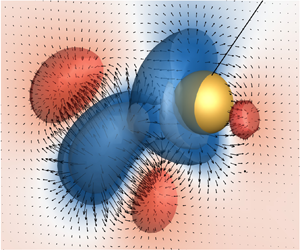
  $m^* = 2.50$. Vectors represent the maximum normalised pressure gradient with a positive direction from low to high. Isosurfaces are based on maximum normalised relative pressure distribution. Red indicates above-reference and blue indicates below-reference pressure zones. (d) Average ( $\kern 0.06em p_{avg}$), maximum ( $\kern 0.06em p_{max}$) and minimum ( $\kern 0.06em p_{min}$) field value of the instantaneous pressure. The blueish band indicates the shedding of the first vortex ring.
Our findings support the hypothesis reported in Young et al. (Reference Young, Li, Capart and Chu2022) for the pendulum trajectory, as we observed a lateral movement of the sphere and vortex structure. More specifically, Young et al. (Reference Young, Li, Capart and Chu2022) reported a dependence of the sphere's lateral displacement on  $m^*$ and $\textit {Re}$, while the trajectories of the shed vortex seem to be insensitive to $\textit {Re}$. This also counts for the pendulum and is a key finding of Gold et al. (Reference Gold, Reiterer, Worf, Khosronejad, Habersack and Sindelar2023), which found that the propagation angle of the shed vortex is independent of $m^*$ and $\textit {Re}$. In addition, herein, we resolved the instantaneous pressure field which features distinct pressure signatures related to the vortex shedding: see figure 6(c).
The deceleration of the sphere, after the vortex was shed, is further supported by the pressure field distribution, in which the pressure gradient vectors point from the low-pressure zone of the detached vortex towards the sphere's wake. We argue that the observed pressure gradient causes momentum transfer from the sphere towards to the vortex structure leading to a deceleration of the sphere. The relatively high-pressure zone in the sphere's front can be attributed to the displacement and drag of the fluid by the sphere towards the wake region. Figure 6(d) shows the average ( $\kern 0.06em p_{avg}$), maximum ( $\kern 0.06em p_{max}$) and minimum ( $\kern 0.06em p_{min}$) field value of the instantaneous pressure. A distinct pressure maximum and even more pronounced minimum are present during the vortex shedding phase. We choose $m^*=2.50$ as the reference case since this density ratio features optimal damping related to FSI, as reported by Gold et al. (Reference Gold, Reiterer, Worf, Khosronejad, Habersack and Sindelar2023).
To investigate the vortex-pressure characteristic regarding different  $\textit {Re}$, we now focus on the below-reference pressure field evolution for $m^*= 2.50, 7.75$ and $14.95$. To do so, we normalise the instantaneous minimum field values of pressure $p_{min}$ by conducting the minimum moving average of the pressure field for all time steps. Doing so, we obtain the non-dimensional pressure field ( $\kern 0.06em p^*_{min}$). In figure 7 we plot the ratio $p^*_{min}/m^*$ against the non-dimensional time $t/T$, where $T$ is the period of oscillation of corresponding $m^*$. As seen in this figure, distinct peaks of various $m^*$ coincide with the peaks of $p^*_{min}/m^*$. The corresponding $t/T$ of the peaks are closer for the denser materials (e.g. $m^*=7.75$ and $14.95$) than the material with smaller density, i.e. $m^*=2.50$. This correlates with the pendulum's velocity, which increases slightly for $m^*\geq 6.00$. Accordingly, the time of vortex separation decreases slightly, $m^*\geq 6.00$ (Gold et al. Reference Gold, Reiterer, Worf, Khosronejad, Habersack and Sindelar2023). At the early stages of motion, i.e. $0< t/T<0.17$, pressure evolution of $m^*=7.75$ and $m^*=14.95$ agree quite well. However, at later times (i.e. at $t/T>0.17$), $p^*_{min}/m^*$ of $m^*=7.75$ decreases more rapidly than that of $m^*=14.95$. Figure 7 further indicates the significant influence of first vortex shedding on the dynamics of the sphere regardless of $m^*$. Plotting the time-averaged vorticity distribution, Gold et al. (Reference Gold, Reiterer, Worf, Khosronejad, Habersack and Sindelar2023) found the maximum pressure on the path of the downward shed vortex, and not in the sphere's wake. This correlates with our analysis of the pressure field highlighting the importance of the pressure field to describe vortex dynamics and vortex–structure interactions.

Figure 7. Pressure characteristics during the first swing for  $m^*=(2.50,3.26,6.00)$. Non-dimensional pressure $p^*$ to $m^*$ ratio plotted against time $t$ to period $T$ ratio. Pressure $p^*$ is the field minimum value normalised by the moving average minimum of 10 data points. For $T$ the oscillation period of the first swing was used. Circles, squares and triangles represent instantaneous values while lines represent a moving average ( $ma_{m^*}$) of 10 data points.
3.2. Drag correction related to vortex shedding and pressure dynamics
Gold et al. (Reference Gold, Reiterer, Worf, Khosronejad, Habersack and Sindelar2023) also found the Strouhal number (Strouhal Reference Strouhal1878) to be a very good estimator to predict the onset of vortex shedding  $t_{vs}$ for the spherical pendulum in a dense fluid. Remarkably, for $m^* < 2$ the model equation (3.2) starts to strongly deviate from the experiments at the instant of vortex separation $t_{vs}$, supporting the above-mentioned vortex interaction mechanism. Hence, a VID correction is suggested. The present VID correction is included in the former drag term and considers additional forces caused by vortex shedding behind the sphere. Mathai et al. (Reference Mathai, Loeffen, Chan and Wildeman2019) approximate the drag coefficient in the presence of vortex shedding as
 \begin{equation} C_{Dvs}=C_D(1+A_z^*\sin\omega_{vs}t), \end{equation}
where  $A_z^*=A_z/D$ is the non-dimensional maximum out-of-plane amplitude (Govardhan & Williamson Reference Govardhan and Williamson1997; Jauvtis, Govardhan & Williamson Reference Jauvtis, Govardhan and Williamson2001; Govardhan & Williamson Reference Govardhan and Williamson2005; Negri et al. Reference Negri, Mirauda and Malavasi2020) and $\omega _{vs}=2{\rm \pi} S_rv_s/D$ is the vortex shedding frequency. Here $S_r$ is the Strouhal number, $v_s$ is the velocity of the sphere and $D$ is the sphere diameter. According to Jauvtis et al. (Reference Jauvtis, Govardhan and Williamson2001) and Govardhan & Williamson (Reference Govardhan and Williamson2005) $A_z^*$ depends on a normalised velocity $v_s^*=v_s/(f_ND)$, where $f_N$ represents the natural frequency of the tethered sphere in water including added mass (Govardhan & Williamson Reference Govardhan and Williamson2005; Eshbal et al. Reference Eshbal, Kovalev, Rinsky, Greenblatt and van Hout2019):
 \begin{equation} f_N=\frac{1}{2{\rm \pi}}\sqrt{\frac{g}{L}\left(\frac{m^*-1}{m^*+m_a^*}\right)}. \end{equation}
 Govardhan & Williamson (Reference Govardhan and Williamson1997) introduced two different modes characterising the VIVs of the tethered sphere facing the uniform flow. The two modes are defined as Mode I and Mode II and occur in a velocity regime of  $v_s^*\sim [5, 10]$ featuring a wide range of normalised amplitudes $A_z^* :[0.2, 0.8]$. Negri et al. (Reference Negri, Mirauda and Malavasi2020) even observed cross-flow oscillation amplitudes up to 1.1 within the first two modes for $m^*=1.38$ and $v_s^*\sim [5, 15]$. In addition, (Jauvtis et al. Reference Jauvtis, Govardhan and Williamson2001) found two more modes (Mode III and IV). Mode III arises in a velocity regime $v_s^* :[20, 40]$. Our experiments fall well within the $v_{s_{max}}^*$ regime of Mode III and we observed $A_z^*$ up to 0.9. We used the values of $A_z^*$ from the recordings of the video camera VC, which are consistent with the findings of Govardhan & Williamson (Reference Govardhan and Williamson1997), Jauvtis et al. (Reference Jauvtis, Govardhan and Williamson2001), Govardhan & Williamson (Reference Govardhan and Williamson2005) and Negri et al. (Reference Negri, Mirauda and Malavasi2020). Table 3 sums up the normalised maximum sphere velocities $v_{s_{max}}^*$ and the corresponding non-dimensionalised maximum out-of-plane amplitudes. The last Mode IV is related to velocities far from those present in this work and is characterised by intermittent bursts of vibration (Jauvtis et al. Reference Jauvtis, Govardhan and Williamson2001). Young et al. (Reference Young, Li, Capart and Chu2022) described the out-of-plane displacement of falling spheres as a consequence of the pressure difference associated with vortex shedding, with small $m^*$ corresponding to higher $A_z^*$. This was also observed in the present findings.
Table 3. Mass ratio  $m^*$, corresponding normalised velocities $v_{s_{max}}^*$ and non-dimensional maximum out-of-plane amplitudes $A_z^*$.

Considering the drag correction introduced in (3.3), the corresponding drag force term is described as  $c_{vs}=C_{Dvs}A_pL/(2V)$. Including this term into (3.2) leads to
 \begin{equation} \left.\begin{gathered} m_{eff}^*\frac{{\rm d}^2\theta}{{\rm d}\tilde{t}^2}={-}k\sin\theta -c_{vs}\left|\frac{{\rm d}\theta}{{\rm d}\tilde{t}}\right|\frac{{\rm d}\theta}{{\rm d}\tilde{t}} -h\left|\cos\theta\right|\textrm{sgn}\left(\frac{{\rm d}\theta}{{\rm d}\tilde{t}}\right), \\ \text{where}\quad c_{vs}=C_D\frac{A_pL}{2V}(1+A_z^*\sin\omega_{vs}t) . \end{gathered}\right\} \end{equation}
 This adaption of the model results in a significant improvement of the model equation for  $m^*< 2$. The model corrections cause a decrease in velocity beginning at the first instant of vortex shedding for $m^*= 1.14$. In addition, the maximum amplitude during the first swing is reduced as shown in figure 8(a). However, in the range of higher mass ratios $m^*>2.0$ the model does not provide any relevant improvement since the amount of damping caused by vortex shedding is small. Figure 8(b) shows the model error for $m^*=7.75$. Therefore, a further correction term related to the wake flow will be introduced.

Figure 8. Amplitude plot of experiment vs model with and without the VID term for (a)  $m^* = 1.41$ and(b) $m^* = 7.75$.
3.3. Wake flow corrections
Mathai et al. (Reference Mathai, Loeffen, Chan and Wildeman2019) present a 2D-PIV-based approach for the improvement of their model by including a term related to the wake flow interaction. Their nonlinear drag model was capable of well predicting the amplitude of motion for the first swing but deviated significantly for subsequent swings. They concluded that the missing part of the model is related to the cylinder entering a disturbed flow field when it first returns. During its swing, the cylinder imparts momentum onto the flow field, which later impacts the bluff body when coming to the turning point. The incoming flow velocity  $U_f$ causes an additional flow resistance (drag) due to the higher relative flow velocity $U_{rel} = v_s - U_f$. From planar 2D-PIV measurements Mathai et al. (Reference Mathai, Loeffen, Chan and Wildeman2019) determined the mean fluid velocity $U_f$ at several different angular positions $\theta$ upstream of the cylinder in small windows of size $2D \times 2D$ through the middle of the cylinder length. Based on a relationship between the normalised fluid velocity $U_f^*$ at normalised angular positions $\theta ^*$, Mathai et al. (Reference Mathai, Loeffen, Chan and Wildeman2019) provided a modified drag term $F_{Df}=1/2\rho _F A_sC_D(v_s - U_f)^2$ for heavy cylinders, where $U_f = U_f^*v_{s0}$. This leads to a new model equation of motion starting at the end of the first swing:
 \begin{equation} m_{eff}^*\frac{{\rm d}^2\theta}{{\rm d}\tilde{t}^2}={-}k\sin\theta -c_{vs}\left|\frac{{\rm d}\theta_{rel}}{{\rm d}\tilde{t}}\right|\frac{{\rm d}\theta_{rel}}{{\rm d}\tilde{t}} -h|\cos\theta|\textrm{sgn}\left(\frac{{\rm d}\theta}{{\rm d}\tilde{t}}\right), \end{equation}
where  $\textrm {d}\theta _{rel}/\textrm {d}\tilde {t} = (v_s - U_f)/\sqrt {Lg}$ denotes the relative angular velocity.
Nevertheless, the LES of a cylinder pendulum with  $m^*= 4.98$ by Worf et al. (Reference Worf, Khosronejad, Gold, Reiterer, Habersack and Sindelar2022) suggest that the influence of the wake already starts before the end of the first swing. This is in line with the present findings with spheres as described previously. The model including the VID does not satisfyingly predict the amplitude and period during the first swing, especially for $m^{*} > 2$. Based on the vortex shedding topology for spherical pendulums, Gold et al. (Reference Gold, Reiterer, Worf, Khosronejad, Habersack and Sindelar2023) suggest starting the model equation (3.6) at the instant $t_{vs}$ when the first vortex sheds. Based on the vortex shedding topology for spherical pendulums presented by Gold et al. (Reference Gold, Reiterer, Worf, Khosronejad, Habersack and Sindelar2023), however, the instant when the first vortex sheds $t_{vs}$ is suggested as the beginning of the model. Further, the findings of Worf et al. (Reference Worf, Khosronejad, Gold, Reiterer, Habersack and Sindelar2022) revealed the significant effect of 3-D flow such as tip vortices. We note that such vortical flow structures are not resolved in the 2-D analysis (see, e.g., Mathai et al. (Reference Mathai, Loeffen, Chan and Wildeman2019)).
In the present study, we analysed the velocity field of the region in front of the sphere  $U_f$ for different angular positions and volumes $V_f$ of size $D^3$ ( $D\times D\times D$). Figure 9(a) shows the data assimilation process at the end of the first swing with angle $\theta _{max}$ and the pendulum velocity $v_s$. Figure 9(b) further shows an extent of the selected fluid volume having a $x$-distance $d_x$ of $1D$ between the centre of $V_f$ and the sphere. To ensure that $V_f$ is on the pendulum's path, the centre of $V_f$ needed to be shifted in the $y$-direction by $d_y = d_x\tan {\theta }$. Depending on the material and different maximum deflection, the number of fluid volumes $n_{V_f}(m^*)$ studied in this work range from $n_{V_f} = 3$ for $m^*= 1.14$ to $n_{V_f}$ = 16 for $m^*= 14.95$. Analogously to Mathai et al. (Reference Mathai, Loeffen, Chan and Wildeman2019), the fluid velocity $U_f$ is normalised by the pendulum velocity at angular position $\theta = 0$, referred to as $v_{s0}$. The corresponding angles $\theta$ are normalised by the maximum angle at the end of the first swing $\theta _{max}$. Since $\theta _{max}$ is negative, $\theta ^*$ is positive when right to equilibrium position with $\theta =0$ and negative if left to it. The data presented in figure 9(c) show a good collapse for all values of $m^*$ and, therefore, a polynomial fit for $U_f^*(\theta ^*)$ is derived. The overall data structure is similar to that presented by Mathai et al. (Reference Mathai, Loeffen, Chan and Wildeman2019). The main difference is the much smaller magnitude of $U_f^*$ for the sphere compared with the cylinder. However, this is what one would expect since a cylinder of the same diameter $D_c = D$ and length $L_c = D$ holds a larger area ( $\kern 0.06em y{-}z$-plane) facing the incoming fluid flow and is generally less streamlined.

Figure 9. (a) Determination of the wake flow velocity  $U_f$ inside the volume $V_f$ of size $D \times D \times D$ at the turning point of the first swing with the peak angular displacement $\theta _{max}$ for $m^*=2.50$. (b) 3-D fluid flow inside $V_f$ interacting with the sphere. (c) Decay of the normalised wake velocity $U_f^*$ vs the normalised angular position $\theta ^*$ for $m^*:[1.14,14.95]$. Note that positive values of $\theta ^*$ indicate movement of the sphere to the left and negative to the right.
When computing (3.6) and varying the initiation time of the wake model, the best fit is found when starting at the instant of shedding of the first vortex presented by Gold et al. (Reference Gold, Reiterer, Worf, Khosronejad, Habersack and Sindelar2023). Finally, the set of equations to describe the dynamics of the subaqueous spherical pendulum can be expressed as
 \begin{equation} m_{eff}^*\frac{{\rm
d}^2\theta}{{\rm d}\tilde{t}^2} = \left\{\begin{array}{@{}ll@{}}
-k\sin\theta -c_{vs}\left|\dfrac{{\rm d}\theta}{{\rm
d}\tilde{t}}\right|\dfrac{{\rm d}\theta}{{\rm d}\tilde{t}}
-h|\cos\theta|\textrm{sgn}\left(\dfrac{{\rm d}\theta}{{\rm
d}\tilde{t}}\right), & t< t_{vs}, \\
-k\sin\theta -c_{vs}\left|\dfrac{{\rm d}\theta_{rel}}{{\rm
d}\tilde{t}}\right|\dfrac{{\rm d}\theta_{rel}}{{\rm
d}\tilde{t}} -h|\cos\theta|\textrm{sgn}\left(\dfrac{{\rm
d}\theta}{{\rm d}\tilde{t}}\right), & t\geq
t_{vs}. \end{array} \right.
\end{equation}
\begin{equation} m_{eff}^*\frac{{\rm
d}^2\theta}{{\rm d}\tilde{t}^2} = \left\{\begin{array}{@{}ll@{}}
-k\sin\theta -c_{vs}\left|\dfrac{{\rm d}\theta}{{\rm
d}\tilde{t}}\right|\dfrac{{\rm d}\theta}{{\rm d}\tilde{t}}
-h|\cos\theta|\textrm{sgn}\left(\dfrac{{\rm d}\theta}{{\rm
d}\tilde{t}}\right), & t< t_{vs}, \\
-k\sin\theta -c_{vs}\left|\dfrac{{\rm d}\theta_{rel}}{{\rm
d}\tilde{t}}\right|\dfrac{{\rm d}\theta_{rel}}{{\rm
d}\tilde{t}} -h|\cos\theta|\textrm{sgn}\left(\dfrac{{\rm
d}\theta}{{\rm d}\tilde{t}}\right), & t\geq
t_{vs}. \end{array} \right.
\end{equation}
This adaption led to a major improvement of the model predictions for both the amplitude and period for  $m^*\in [1.14, 14.95]$. Figure 10(a) compares the model with the VID correction against the model with both the VID correction and the wake ( $\textrm {WF}+\textrm {VID}$) correction. As can be seen, we also plot the measured results of $m^* = 2.50$. As seen, the comparisons mark an excellent fit between the $\textrm {WF}+\textrm {VID}$ model and the experimental data over the entire duration of the experiment. In addition, we plot in figure 10(b) the angular displacement of the pendulums, $\theta$, vs the angular velocity, $\omega _s$. Again, as can be seen in this figure, it seems that the $\textrm {WF}+\textrm {VID}$ model outperforms the VID model significantly. In addition, this is clearly evident in figure 11(a) in which the absolute amplitude errors in rad for both the $\textrm {WF}+\textrm {VID}$ and the VID model are displayed. In particular, as $m^*$ increases, the wake correction leads to higher model accuracy. Finally, in figure 11(b) we plot the time history of the relative amplitude error. In contrast to the absolute error values, the maximum relative errors relate to the lighter materials. However, one has to take into account that the pendulums with small $m^*$ can solely induce minor deflection angles and, thus, absolute errors would be limited. As a result, the maximum relative error is associated with the pendulum with $m^*=1.14$. This maximum error is $\sim$35 % which corresponds to an absolute amplitude error of 0.015 rad. By including the wake correction in the VID model, the mean relative error decreased from 38 % to 7 %. Hence, the proposed model (3.7) allows for, with a high level of confidence, predictions of the 3-D FSIs related to the subaqueous pendulum for a wide range of $m^*$.

Figure 10. (a) Amplitude plot of experiment vs model with ( $\textrm {WF}+\textrm {VID}$) and without (VID) the wake correction for $m^* = 2.50$. (b) Shell plot of experiment vs model with ( $\textrm {WF}+\textrm {VID}$) and without (VID) the wake correction for $m^* = 2.50$. Note that $\omega _s$ is the angular velocity and $\theta$ is the angle of displacement.

Figure 11. (a) Amplitude error of the VID and the  $\textrm {WF}+\textrm {VID}$ models in rad for $m^* = 1.41$ and 14.95.(b) The relative error in the peak amplitude before (VID) and after including the history force due to wake flow ( $\textrm {WF}+\textrm {VID}$). The dashed lines represent the mean relative errors for the two models (blue, $\textrm {VID} = 38\,\%$; red, $\textrm {WF}+\textrm {VID} = 7\,\%$). The coloured bands indicate a range from the mean relative error $\pm$ and the standard deviation $\sigma$ for VID (blue) and $\textrm {WF}+\textrm {VID}$ (red).
3.4. Perspective on flexible bodies, low Reynolds numbers and buoyant particles
The presented wake model is found to be applicable for the wide range of  $m^*$ and $A_z^*$ investigated in the present study of heavy spheres, as well as the stiff cylinder pendulum from Mathai et al. (Reference Mathai, Loeffen, Chan and Wildeman2019) which allows for small out-of-plane movement. In comparison with rigid cylinders, flexible cylinders can exhibit more complex structural response and vortex-wake patterns (Ma et al. Reference Ma, Lin, Fan, Wang and Triantafyllou2022). These can significantly alter the damping behaviour due to a net energy transfer between fluid and the body. In addition, the added mass effects can be both positive and negative (Ma et al. Reference Ma, Lin, Fan, Wang and Triantafyllou2022; Modarres-Sadeghi Reference Modarres-Sadeghi2022). The fact that the self-excited flow field of the pendulum is unsteady, makes it even more complex and until now there is only limited research on flexible cylinders in unsteady flow (Ma et al. Reference Ma, Lin, Fan, Wang and Triantafyllou2022). The cylinder can experience different flow velocities along its axis and therefore can lock-in with the flow at different points, forcing the structure to oscillate (Modarres-Sadeghi Reference Modarres-Sadeghi2022). To adapt our model to flexible bodies, the introduction of additional model terms capturing the bodies’ mechanical properties (e.g. the Cauchy number) could be promising. For a flexible cylinder, further adaptations could be the inclusion of the dimensionless damping parameter $c^*$ by Vandiver, Ma & Rao (Reference Vandiver, Ma and Rao2018), which places the global structural response on a spectrum of lightly to heavily damped systems (Ma et al. Reference Ma, Lin, Fan, Wang and Triantafyllou2022).
Regarding the limitations of this study for small Reynolds numbers, there are various aspects to consider. As concluded by Dolfo et al. (Reference Dolfo, Vigué and Lhuillier2020), the domain of small Reynolds numbers  $\textit {Re} \ll 1$ is easily observed with micrometre-sized particles, but the particle size limits considerably the range of $St$ numbers that can be investigated. However, with macroscopic objects, it is difficult to obtain small $\textit {Re}$, but a large range of $St$ is easily available (Dolfo et al. Reference Dolfo, Vigué and Lhuillier2020). To examine the response time of the spheres, we calculate the Stokes number, $St = t_s v_s/L_s$, where $t_s$ is the relaxation time of the bob mass ( $=\rho _s D^2/ (18\mu )$), where $\mu$ is the dynamic viscosity of the fluid ( $10^{-3}$ Pas), $v_s$ is the bulk velocity (i.e. maximum velocity of the pendulums) and $L_s$ is a characteristic length of the flow (i.e. the pendulum length $L$). This gives $St\in [4, 400]$ with $\textit {Re} \in [10^3, 10^4]$ and $St$ and $\textit {Re}$ increase with increasing $m^*$. Alternatively, we can calculate $St$ based on the pendulum period $St = t_s/T$ which gives us $St\in [2, 150]$. As predicted by Stokes (Reference Stokes1851), Dolfo et al. (Reference Dolfo, Vigué and Lhuillier2020) found a quadratic dependence of the measured drag force with the sphere radius, if the sphere radius is larger than the viscous penetration depth. In addition, the value of the drag force was in very good agreement with Stokes’ result (Dolfo et al. Reference Dolfo, Vigué and Lhuillier2020). Regarding the cylindrical pendulum, the results for large aspect ratios (cylinder length to diameter $L_c/D_c = 52$) are remarkably close to Stokes’ theory, whereas for $L_c/D_c = 13.3$ the finite-length cylinder theory fits best (Dolfo et al. Reference Dolfo, Vigué and Lhuillier2021). In the domain of small $St$ and small $\textit {Re}$, where $C_D = 24/\textit {Re}$, fluid damping (fluid viscosity) effects (Chen Reference Chen1981) are dominant to characterise the motion of the spherical pendulum. For moderate Reynolds numbers, as studied by Bolster et al. (Reference Bolster, Hershberger and Donnelly2010), to the range of $\textit {Re}$ of this study, effects such as vortex shedding and Reynolds drag become significant.
For buoyant spheres, where the added mass  $m_a$ contributes significantly to the particle's inertia, the model corrections regarding VID and wake interactions might require adaptation. In addition, inertial heavy and light particles tend to behave differently in turbulent flows (Toschi & Bodenschatz Reference Toschi and Bodenschatz2009). Heavy particles are expelled from vortical regions, whereas light particles are drawn into them (Calzavarini et al. Reference Calzavarini, Cencini, Lohse and Toschi2008a,Reference Calzavarini, Kerscher, Lohse and Toschib; Toschi & Bodenschatz Reference Toschi and Bodenschatz2009; Vajedi et al. Reference Vajedi, Gustavsson, Mehlig and Biferale2016). The latter is described as a consequence of pressure gradient forces in the fluid field (Vajedi et al. Reference Vajedi, Gustavsson, Mehlig and Biferale2016). This might influence the FSIs of macroscopic buoyant spherical pendulums and points out the need for further research.
4. Conclusion
In this work, a detailed analysis concerning the FSI of heavy spherical pendulums underwater is presented for a wide range of solid-to-fluid mass ratios  $m^*$ of the pendulums. The interactions of various pendulums with their surrounding flow fields are investigated using the measured data from DOT, tr-3D-PTV and PTV. The experimental data obtained from these tests marks a strong dependency of the amplitude and the oscillation frequency of pendulums on the solid-to-fluid mass ratio $m^*$. Furthermore, the influence of VID oscillation was clearly evident. In particular, for low values of $m^*$, vortex shedding and the resulting oscillating drag significantly affect the pendulums’ decay. A short propulsion of the sphere, followed by distinct deceleration was observed during vortex separation. We analysed the pressure associated with the vortex shedding and its relevance for out-of-plane displacement of the pendulums. In addition, analogies between pressure effects regarding the present pendulum and the falling sphere experiments by Young et al. (Reference Young, Li, Capart and Chu2022) are discussed.
The findings revealed that disturbed flow fields around pendulums significantly influence their oscillations. As a result, we revised the theory-based equation of motion of underwater pendulums, which was proposed by Mathai et al. (Reference Mathai, Loeffen, Chan and Wildeman2019), to include both oscillating drag and the wake interaction for a more accurate prediction of the spherical pendulum motion. Further, based on our experimental tests, we implemented a wake model initiation, at the instant when the first vortex is shed, to address the open research question raised by Worf et al. (Reference Worf, Khosronejad, Gold, Reiterer, Habersack and Sindelar2022).
The added mass value of the implemented model was equal to the potential flow theory value of  $m_a=0.5$. Literature-based drag coefficients as a function of $\textit {Re}$ (Hoerner Reference Hoerner1965; Roos & Willmarth Reference Roos and Willmarth1971; Schlichting & Gersten Reference Schlichting and Gersten2017) were used in the model equation to enhance its agreement with the experimental tests. We show that implementing both drag and wake correction can clearly reduce errors in the frequency and amplitude of oscillation and, thus, significantly improve the quality of the proposed model. As a result of these improvements, the proposed model equation (3.7) is capable of predicting, with an unprecedented level of confidence, the 3-D FSIs for a wide range of solid-to-fluid mass ratios and Reynolds numbers. Overall, this highlights the importance of knowing the underlying mechanisms such as added mass, nonlinear drag and vortex dynamics to better understand the interaction between the fluid and structures.
While the present model is valid for rigid bluff bodies of circular cross section, an extension for other geometries or flexible bodies (e.g. flexible cylinders) requires more research on the complex FSI in unsteady flow. In particular, investigations on the complex wake interactions are needed. This can be done in the style of the present 3D-PTV wake analysis and it can help to find models for other bluff bodies, and/or for the validation of numerical FSI/immersed boundary models for flexible bodies, oscillating in unsteady flow.
We want to stress the importance of research on buoyant particles in turbulence, potentially based on the buoyant spherical pendulum. Therefore, the methodological framework of the present study and the deduced model approaches are potentially beneficial, especially to investigate the role of pressure gradient forces. Further, investigating the dynamics of heavy and buoyant pendulums in different viscous fluids and for small Reynolds numbers could be a promising continuation of this topic.
In future research, we will employ the implemented model equation to describe the impact properties in the study of particle–wall and particle–particle collisions with a pendulum apparatus. Once again, the findings of the present paper highlight the key role of pendulum investigation in addressing fundamental questions in fluid dynamics research.
Supplementary material and movie
Supplementary material and movie are available at https://doi.org/10.1017/jfm.2023.1008.
Acknowledgements
Financial support by the Austrian Science Fund and the Austrian Federal Ministry for Digital and Economic Affairs and the National Foundation of Research, Technology, and Development of Austria, and the Christian Doppler Research Association is gratefully acknowledged. The authors thank LaVision GmbH for the support with the pressure from PTV software package.
Funding
This research was funded by the Austrian Science Fund FWF P33493 (T.G., K.R., D.W., H.H. and C.S.); the Christian Doppler Research Association (T.G., K.R. and D.W.) and the Austrian Federal Ministry for Digital and Economic Affairs and the National Foundation of Research, Technology, and Development of Austria (T.G., K.R. and D.W.).
Declaration of interests
The authors report no conflict of interest.
Data availability statement
The datasets analysed during the current study can be made available from the corresponding author on reasonable request.


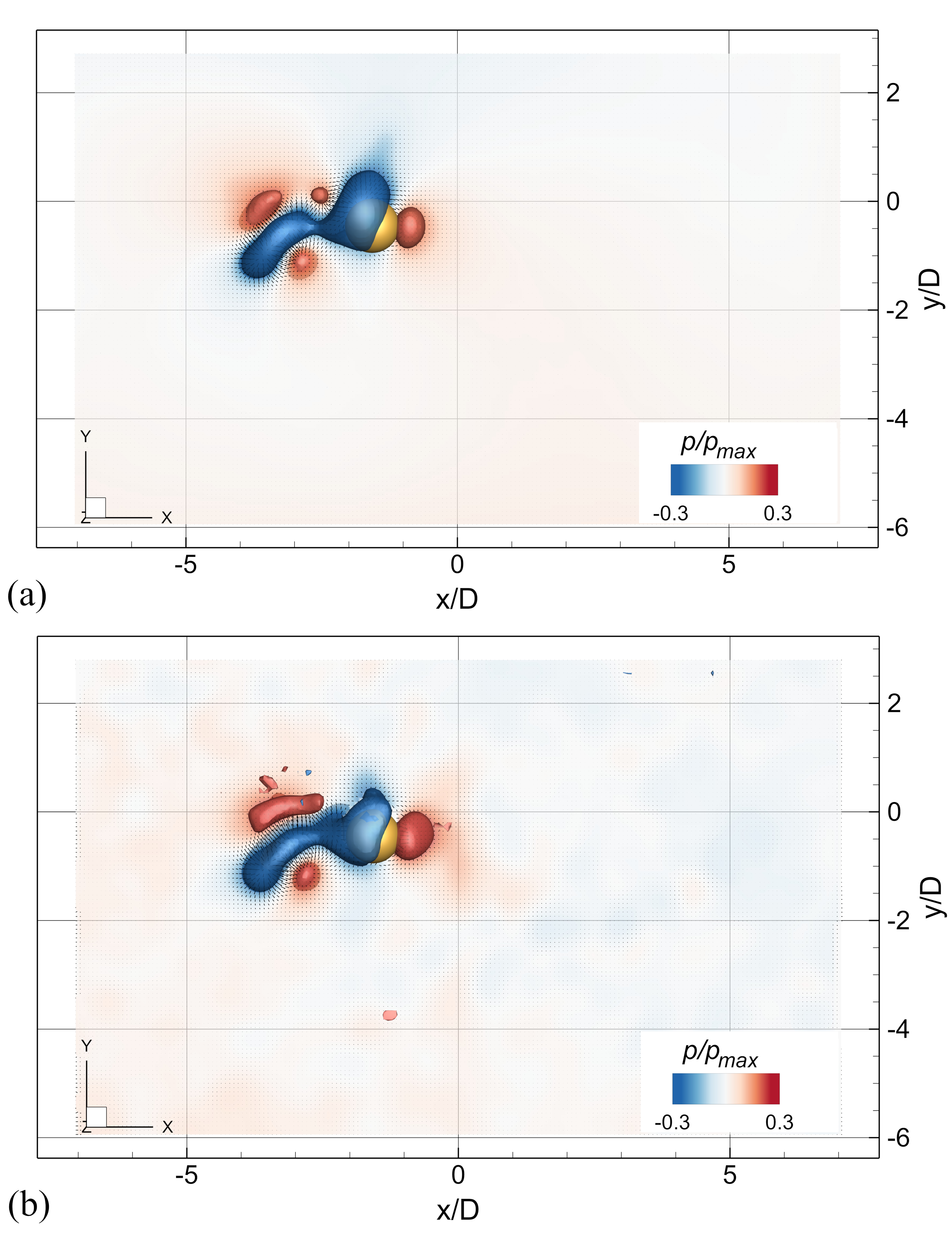

 Open access