


1. Introduction
Unsteady three-dimensional (3-D) flow separation is a ubiquitous phenomenon that can be observed in flows both in nature as well as in engineering. Examples include the swimming of fish (Zhang et al. Reference Zhang, Huang, Pan, Yang and Huang2022), birds and aircraft experiencing gusts (Cheney et al. Reference Cheney, Stevenson, Durston, Song, Usherwood, Bomphrey and Windsor2020), or even rapid submarine manoeuvring (Bettle, Gerber & Watt Reference Bettle, Gerber and Watt2009). To-date, many studies on unsteady flow separation have focused on two-dimensional (2-D) flow separation (Yu et al. Reference Yu, Amandolese, Fan and Liu2018; Li et al. Reference Li, Feng, Kissing, Tropea and Wang2020; Miotto et al. Reference Miotto, Wolf, Gaitonde and Visbal2022). With regards to 3-D separation, most studies have restricted themselves to investigations of complex separation mechanics with steady boundary conditions. One common canonical test case is that of the 6:1 prolate spheroid due to the abundance of complex flow features that occur even at small incidence angles. The transition of the boundary layer to turbulence (Wetzel Reference Wetzel1996), pressure-gradient induced separations (El Khoury, Andersson & Pettersen Reference El Khoury, Andersson and Pettersen2012) and helical vortex formations (Jiang et al. Reference Jiang, Andersson, Gallardo and Okulov2016) are but a few phenomena that have been extensively studied using the prolate-spheroid geometry. However, for highly unsteady, 3-D separating flows, a limited amount of studies exist. As such, many aspects of dynamic 3-D flow separation processes have not been explored. For instance, how the 3-D separated flow around a prolate spheroid reacts to a sudden change in boundary conditions has not yet been considered. To gain a deeper understanding of how unsteadiness affects separating 3-D flows, we use the well-characterized 6:1 prolate spheroid and investigate how the separated wake and the surface pressure distribution are influenced by acceleration and deceleration.
1.1. Background on flow separation
Flow separation has often been categorized into two categories: separation due to an abrupt change of the geometry and detachment on flat (or mildly curved) surfaces owing to the existence of a strong adverse pressure gradient (APG) (Deck Reference Deck2012). The former category is characterized by its fixed separation location. Classical examples include the backward-facing step (Le, Moin & Kim Reference Le, Moin and Kim1997), splitter plate (Hwang, Yang & Sun Reference Hwang, Yang and Sun2003) or an inclined flat plate (Stevenson, Nolan & Walsh Reference Stevenson, Nolan and Walsh2016). In contrast, the separation induced by an APG on a smooth surface is relatively complex due to its intermittent behaviour; the locations of separation and reattachment vary due to disturbances in the pressure-gradient field (Simpson, Chew & Shivaprasad Reference Simpson, Chew and Shivaprasad1981). The flow within a diffuser (Elyasi & Ghaemi Reference Elyasi and Ghaemi2019), the flow around an airfoil (Ma, Gibeau & Ghaemi Reference Ma, Gibeau and Ghaemi2020) or the flow around a prolate spheroid (Jiang et al. Reference Jiang, Andersson, Gallardo and Okulov2016) all belong to the above category.
For smooth geometries with intermittent separation (APG induced), the definition of the separation location depends on whether the flow is two-dimensional or three-dimensional in nature. For 2-D flow separation, Prandtl (Reference Prandtl1904) derived a criterion based on the no-slip boundary condition, implying that the flow separates at a point with zero wall shear and the skin friction admits a negative gradient. For unsteady boundary conditions, the separation point may move (Rott Reference Rott1956; Moore Reference Moore1958; Sears & Telionis Reference Sears and Telionis1971; Haller Reference Haller2004). More recently, Lamarche-Gagnon & Vétel (Reference Lamarche-Gagnon and Vétel2018) observed the moving separation point in a rotor-oscillator flow using a cylinder in non-periodic transitions.
In 3-D flows, however, separation occurs along lines, and not at points of zero skin-friction (Tobak & Peake Reference Tobak and Peake1982; Simpson Reference Simpson1995; Délery Reference Délery2001). After the first studies on 3-D separation published by Legendre (Reference Legendre1952), a heuristic 3-D flow separation criterion was then proposed by Lighthill (Reference Lighthill1963), who hypothesized that separation lines originate from regions of zero skin friction and that the separation line must be a closed curve. Wang (Reference Wang1972, Reference Wang1974) listed some examples where Lighthill's rule does not apply and where the separation line and zero skin-friction regions do not coincide. Wang (Reference Wang1976) further distinguishes between open and closed separation. For a closed separation, the separation line is closed upstream of the separation, preventing the upstream flow entering the separated area; see for example figure 1(a). In contrast, for an open separation, the limiting streamlines run directly into the separated region; see figure 1(b). More detailed criteria of steady 3-D flow separation were derived by Wu et al. (Reference Wu, Tramel, Zhu and Yin2000), Wu, Ma & Zhou (Reference Wu, Ma and Zhou2007) and Surana, Grunberg & Haller (Reference Surana, Grunberg and Haller2006). These studies clearly distinguish between open and closed separation zones. Four possible separation line signatures are thus summarized: saddle nodes; saddle-limit cycles; saddle spirals and limit cycles (Surana et al. Reference Surana, Grunberg and Haller2006).

Figure 1. (a) Example of a closed separation with closed separation line. (b) A case with open separation with two open separation lines. (c) For an accelerating sphere, the separation line moves backwards in the subcritical  $Re$ range (Fernando et al. Reference Fernando, Marzanek, Bond and Rival2017). (d) For an accelerating delta wing, the flow has been observed to reattach on the wing surface (Marzanek & Rival Reference Marzanek and Rival2019). In contrast, for an accelerating prolate spheroid, a number of scenarios are possible: (e) the separation line will move closer to the model meridian centre or (f) a reattachment line will be created. Sketches in panels (g) and (h) illustrate possible scenarios for decelerations. To make the panels clear, the possible larger cross-flow separation for decelerations is only presented on one side of the model body.
1.2. Examples of unsteady 3-D flow separation
A simple example of unsteady 3-D separation occurs for the flow around a sphere, as illustrated in figure 1(c). Owing to the axisymmetry of the problem, the flow shows very similar features to that of the 2-D problem of the flow separation around a cylinder. Under subcritical conditions, Fernando et al. (Reference Fernando, Marzanek, Bond and Rival2017) confirmed that the separation line on a sphere moves downstream during acceleration, which is consistent with the moving characteristic of the APG-induced flow separation observed for 2-D problems. The phenomenon of moving separation lines was explained via theoretical considerations based on the unsteady potential-flow solution around an accelerating sphere. Specifically, in unsteady potential flow, the pressure-gradient field around a sphere shifts from adverse to favourable for strong accelerations.
Moving on to fully 3-D separated flows, the flow over delta wings has been widely studied (Gursul Reference Gursul2005). On a delta wing at high incidence angles, two large, counter-rotating vortices roll up from the leading edges (separation lines) on the wing suction side. Note that the separation line lies very close to the wing apex for a thick delta wing with rounded leading edges (Délery Reference Délery2001). Even in unsteady flows, dynamic motions do not change the location of the separation line on a delta wing significantly (Gursul Reference Gursul2005). However, unsteady kinematics influence other flow features, such as the changing position of the vortex centre and varying locations of vortex breakdown (Lowson & Riley Reference Lowson and Riley1995; Délery Reference Délery2001; Mitchell & Délery Reference Mitchell and Délery2001). Marzanek & Rival (Reference Marzanek and Rival2019) studied the effects of streamwise acceleration on the flow around a non-slender delta wing at various incidence angles. Although the separation line was fixed, as sketched in figure 1(d), the separated flow would reattach on the wing suction side during strong accelerations. Surface pressure measurements confirmed that the reattachment coincided with a strong favourable pressure gradient (FPG) during acceleration. Note that for some kinematics, the reattachment of the flow prevailed long after the acceleration ended and a memory effect of the flow was observed resulting in a period of sustained lift (Marzanek & Rival Reference Marzanek and Rival2019). Here, the term memory effect indicates the flow is still influenced significantly by events that occurred in the past (Zhou & Antonia Reference Zhou and Antonia1995; Kriegseis, Kinzel & Rival Reference Kriegseis, Kinzel and Rival2013; Mamba & Magniez Reference Mamba and Magniez2018).
With regards to non-fixed separation lines, the 6:1 major–minor ratio prolate spheroid has been a widely used benchmark model under steady conditions (Wetzel Reference Wetzel1996; Wetzel, Simpson & Chesnakas Reference Wetzel, Simpson and Chesnakas1998; Surana et al. Reference Surana, Grunberg and Haller2006; Wu et al. Reference Wu, Ma and Zhou2007). Similar to the flow over a delta wing, on an inclined prolate spheroid, a pair of counter-rotating primary vortices originate from separation lines. The separation can be explained by the existence of strong circumferential pressure gradients (Han & Patel Reference Han and Patel1979; Tobak & Peake Reference Tobak and Peake1982), which is caused by the prolate spheroid surface curvature. The location of the separation lines influences the size of the wake and, therefore, significantly impacts the hydrodynamic loads. In steady conditions, the locations are attributed to the incidence angle ( $\alpha$),
  $Re$ and the local body radius (Jeans & Holloway Reference Jeans and Holloway2010; Lee Reference Lee2018). For unsteady conditions, Wetzel (Reference Wetzel1996) conducted measurements on a pitching prolate spheroid. The circumferential skin friction distributions on the model surface were measured via hot film sensors and the locations of minimum skin friction were used to define the separation lines. Movement of the separation lines in a circumferential direction was observed during the pitching manoeuvre, especially at higher incidence angles. However, due to the limitations in the measurements, the dynamic cross-flow patterns have not been presented.
1.3. Objectives
For the case of an inclined prolate spheroid, it remains unclear how the separated flow will vary during acceleration. In particular, the location of the separation line and the vorticity distribution in the cross-flow are likely to be affected by model acceleration and deceleration, as illustrated in figure 1(e–h). Similar to the aforementioned studies of spheres and delta wings, it can be expected that an FPG will form in the rear section of an inclined prolate spheroid during strong accelerations. Thus, it is hypothesized that the separation line will move closer to the model meridian; see figure 1(e). Similar to the dynamic flow on a delta wing, a strong FPG could mitigate the cross-flow structures and even lead to local reattachment near the model meridian; see figure 1(f). In contrast, for a decelerating prolate spheroid, the separation line could either move outwards (figure 1g) or persist at its original location as the steady condition (figure 1h), both resulting in larger cross-flow structures due to an increased APG during deceleration. However, it remains to be seen which of the possible flow features will occur, and how the interplay of vortical structures and surface pressure distribution will affect the separation and reattachment processes.
In addition to the initial response of the cross-flow to an acceleration, the resulting evolution of the separated structures is also of interest. Kriegseis et al. (Reference Kriegseis, Kinzel and Rival2013) observed minimal memory effects from the initial attached boundary-layer vorticity to the subsequent vortex formation process on an accelerating plate. However, leading-edge vortex (LEV) formation, followed by the later shedding of the LEV, has led to an unsteady flow condition up to 14 chord lengths after acceleration (Mancini et al. Reference Mancini, Manar, Granlund, Ol and Jones2015). While the exact formation time, vorticity strength and vortex stability for the LEV are dependent on plate kinematics, other studies confirmed the existence of memory effects on accelerating plates (Onoue & Breuer Reference Onoue and Breuer2016; Kaiser, Kriegseis & Rival Reference Kaiser, Kriegseis and Rival2020). As discussed earlier, a different type of memory effect was observed on a non-slender delta wing. Marzanek & Rival (Reference Marzanek and Rival2019) reported a reattachment of the separated flow, which persisted even after the acceleration was completed. With regards to the inclined, accelerated prolate spheroid investigated in the present study, it is hypothesized that the separated cross-flow will also be altered for a certain distance travelled before recovery to the fully separated state. However, as the separation is open and dominated by a strong helical vortex, we expect a rapid recovery of the separated region compared with that of a (statistically) steady flow.
Therefore, the objectives of the current study are two-fold. First, we strive to understand the dynamic separation mechanics of the 3-D flow on a prolate spheroid under axial accelerations and decelerations, by capturing the separation lines and the cross-flow patterns. Furthermore, the memory effects resulting from the dynamic motions will be investigated. The present study is organized as follows. The experimental methods and model kinematics are first presented in § 2. The results of instantaneous pressure distributions, dynamic flow separation and circulation histories are then presented and discussed in § 3. Finally, conclusions and practical implications of the current study are summarized in § 4.
2. Experimental methods
A description of the prolate-spheroid model and the experimental methods are presented in § 2.1. Thereafter, a detailed description of the model kinematics is provided in § 2.2.
2.1. Experimental set-up
All experiments were performed in a  $15$-m-long towing tank with a
  $1\ {\rm m} \times 1\ {\rm m}$ cross-section. Three sides of the tank allow for optical access through glass panels and the top of the tank is equipped with a slotted ceiling to allow for the connection between a high-speed traverse above the tank and the model while minimizing free-surface effects. Figure 2(a) presents the 6:1 prolate spheroid model with length
  $L=1000$ mm and the maximum diameter of
  $D=166.7$ mm. The model was printed using acrylonitrile butadiene styrene (ABS), and subsequently sanded, treated with several layers of epoxy and then finished with two layers of flat-black paint to ensure a smooth surface with low reflectivity. A rear-mounted cylindrical sting connected the model to a high-speed traverse located above the tank. The model was towed at three incidence angles
  $\alpha \in \{10^\circ, 15^\circ, 20^\circ \}$, leading to a maximum blockage ratio of
  $4.9\,\%$ at
  $\alpha =20^\circ$. Thus, blockage effects are considered to be negligible here.
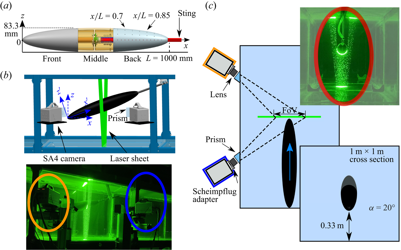
Figure 2. (a) Schematic of a 1-m-long 6:1 prolate-spheroid model and picture of the model; (b) side view of the time-resolved stereoscopic particle image velocimetry (sPIV) camera set-up consisting of two Photron SA4 cameras; and (c) top view of the set-up showing the moving prolate spheroid passing through the stationary laser sheet.
Multiple pressure ports each with a diameter of  $1.6$ mm are located in the back half of the model. The pressure ports are spaced
  $0.05L$ in the longitudinal direction and located between
  $x/L=0.6$ and
  $x/L=0.95$. Along the circumferential direction, the ports are placed at
  $\theta \in \{ 0^\circ,30^\circ,60^\circ,90^\circ \}$ with
  $\theta =0^\circ$ being the top (meridian centre) of the model. Owing to the symmetry of the body, only some of the pressure ports were used in the current study. Among the various sensors, eight Omega PX419 absolute pressure sensors were used. These sensors have a range of
  $6.89$ kPa and an overall uncertainty of
  $0.08\,\%$ of full scale. The pressure data were acquired at a frequency of
  $1$ kHz using a National Instruments USB-6212 DAQ system. The pressure data were normalized, leading to the pressure coefficient
 \begin{equation} C_p=\frac{p-p_\infty}{0.5 \rho U_{II}^2}, \end{equation}
where  $p$ is the instantaneous pressure measured at the pressure tap when the model is moving and the reference pressure
  $p_\infty$ is the static pressure far away from the body. The term
  $0.5\rho U_{II}^2$ is the dynamic pressure defined by the constant post-acceleration velocity
  $U_{II}$. The overall sensor uncertainty corresponds to an expected measurement error of
  $\pm 0.005 C_p$. The pressure data were ensemble-averaged over ten distinct runs.
To quantify the development of the cross-flow separation, we used a time-resolved stereoscopic particle image velocimetry (sPIV) system. Laser sheet and cameras were fixed, while the model was towed through thus allowing for a scanning reconstruction; see the work of Bond et al. (Reference Bond, Marzanek, Neeteson and Rival2019). Figure 2(b,c) shows a schematic of the sPIV set-up. The water was seeded with 60- $\mathrm {\mu }$m polyamide particles. The flow field was illuminated with an approximately
  $1.5$-mm-thick laser sheet generated via a
  $40$-mJ-per-pulse Photonics Nd-YLF high-speed laser through a series of cylindrical lenses. The imaging system consisted of two Photron Fastcam SA4 cameras (
 $1024 \times 1024$ pixels), each equipped with a
  $60$-mm Nikkor lens and Scheimpflug adapters to ensure a sharp image for the entire measurement plane. A photoelectric sensor (CY-122B-P) was mounted to the towing tank and was used to trigger the recording of the sPIV system on half a model length before the acceleration. As such, synchronization between model kinematics and recording was ensured, and the acquired velocity fields were ensemble averaged. The sPIV system was operated at a frequency of
  $2000$ Hz. Water-filled prisms were mounted on the tank to eliminate optical distortions as the cameras were installed at a slanted angle to the tank wall (Prasad & Jensen Reference Prasad and Jensen1995; Raffel et al. Reference Raffel, Willert and Kompenhans1998; Van Doorne & Westerweel Reference Van Doorne and Westerweel2007). The field of view (FoV), as labelled in figure 2(c), was approximately
  $2D\times 1.5D$ in size for all experiments. In the stereoscopic calibration procedure, a two-sided multi-plane calibration target featuring a regular grid of markers was used. The self-calibration method in DaVis 8.4.0 was employed to correct for possible misalignment between the calibration plate and the laser light sheet. A multi-pass cross-correlation algorithm and fixed final interrogation window size of
  $32\times 32$, with 50 % overlap, was used in post-processing (Soria Reference Soria1996). The particle image diameters were, on average, approximately 3 pixels. The spatial resolution of in-plane vectors was fixed at
  $3.6$ mm. Every second recorded frame was dropped to ensure sufficient particle displacements in the cross-correlation step. The final out-of-plane displacement between correlated frames was in the range of 1–1.5 mm, corresponding to
 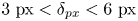 $3\ \mathrm {px}<\delta _{px}<6\ \mathrm {px}$. Assuming a correlation accuracy of
  $\epsilon _{ip}=0.1$ px (Raffel et al. Reference Raffel, Willert and Kompenhans1998) for the in-plane displacement, an in-plane velocity estimation error in the range of
  $1.7\,\% < e_{ip} =\epsilon _{ip}/\delta _{px} < 3.3\,\%$ is expected for the present camera set-up. According to the work of Lawson & Wu (Reference Lawson and Wu1997), the out-of-plane velocity error is approximately
  $2\,\% < e_{op}< 3.9\,\%$. The velocity fields were then ensemble-averaged over 20 runs to further improve the measurement accuracy.
2.2. Kinematics
An  $Re$ range was selected where the observed flow structures remain similar (Guo, Kaiser & Rival Reference Guo, Kaiser and Rival2023). Weak
  $Re$ scaling was observed for steady flow in the range of
  $1.0\times 10^6\leq Re \leq 1.5\times 10^6$. The separation line locations as well as the vorticity distribution were observed to be very similar in this
  $Re$ range. Therefore, in the present study, the model was accelerated from the initial velocity
  $U_{I} = 1.0$ m s
 $^{-1}$ (
 $Re =1.0\times 10^6$) to the final constant velocity
  $U_{II} = 1.5$ m s
 $^{-1}$ (
 $Re =1.5\times 10^6$). In contrast, the model was decelerated from
  $U_{II} = 1.5$ m s
 $^{-1}$ to
  $U_{I} = 1.0$ m s
 $^{-1}$, so as to ensure a range of
  $1.0\times 10^6\leq Re \leq 1.5\times 10^6$ for both dynamic motions. The acceleration modulus is defined as
 \begin{equation} a^*=\frac{a_s L}{(U_{II}-U_{I})^2}, \end{equation}
where  $a_s$ is the physical acceleration. In the current study, the three acceleration moduli are
  $a^* \in \{ 2, 4, 6 \}$, and the three deceleration moduli are
  $a^* \in \{-2, -4, -6\}$, all tested at three incidence angles
  $\alpha \in \{10^\circ$,
  $15^\circ$,
  $20^\circ \}$. An alternative metric to characterize the unsteadiness of the problem is the reduced frequency:
 \begin{equation} k=\frac{{\rm \pi} f D}{U_{II}}, \end{equation}
where  $f=1/T$ is the imposed frequency and
  $T$ is the acceleration period. The three reduced frequencies
 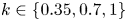 $k \in \{ 0.35, 0.7, 1 \}$ correspond to the three accelerations
  $a^* \in \{ 2, 4, 6 \}$.
2.3. Scanning PIV for unsteady flows
Capturing an unsteady flow with a stationary time-resolved scanning sPIV system requires special attention as the model is accelerating while moving through the high-speed laser sheet. As such, the measurement section relative to the model and the time instance that is captured change simultaneously. As mentioned above, every second frame was dropped during the sPIV correlation to ensure sufficient particle displacement, leading to a time step of  $\Delta t=0.001$ s. The model displacement between two consecutive frames was
  $\Delta x_{max} \approx 1.5$ mm and the velocity change of the model was
  $\Delta U \leq 0.15\,\% U_{II}$. Therefore, the distortion of the acquired velocity fields due to the ratio of data acquisition and flow time scales is small.
To allow for a more complete analysis of the unsteady 3-D flow, the same kinematics were repeated multiple times with different physical starting positions of the model in the towing tank. As the laser sheet location was fixed, starting the acceleration earlier or later allowed one to capture a different stage of the dynamic process via the sPIV set-up, as explained by Bond et al. (Reference Bond, Marzanek, Neeteson and Rival2019). In figure 3, the instantaneous velocity ( $U_{inst}$) is plotted against the dimensionless distance (
 $x/L$) for
  $a^*=6$ and
  $a^*=-6$. Three different acceleration end positions are selected such that the acceleration ends when the laser sheet hits the model at
  $x/L=0.5$ (
 $A_{0.5L}$),
  $x/L=0.75$ (
 $A_{0.75L}$) and
  $x/L=1.0$ (
 $A_{1.0L}$). The sPIV data were always evaluated for the rear section of the model (
 $0.6\leq x/L \leq 1.0$), as the flow separation in this region was of the highest interest.

Figure 3. (a) Instantaneous velocity  $U_{inst}$ plotted against the dimensionless distance travelled (
 $s^*$) for the largest acceleration modulus
  $a^*=6$ and the largest deceleration modulus
  $a^*=-6$. (b) 3-D schematic showing model acceleration relative to the measurement volume.
To further clarify the details of the measurements, a 3-D perspective of the model at  $\alpha =20^\circ$ is depicted in figure 3(b). In the body-fixed coordinate system, the three cases
  $A_{1.0L}$,
  $A_{0.75L}$ and
  $A_{0.5L}$ are highlighted. Specifically, the
  $A_{1.0L}$ case indicates that when the rear section of the model passes through the laser sheet, the model begins accelerating and the early evolution of the dynamic flow structures is captured. The
  $A_{0.75L}$ case represents the acceleration starting earlier and thus the flow captured here is shortly after the acceleration. For the
  $A_{0.5L}$ case, the flow structures were already influenced by the acceleration over a significant amount of time (around half of the model length) and the acceleration ended before data acquisition in this rear region of the model began. The three different measurement volumes thus allow us to examine how quickly the flow reacts to the model acceleration and how quickly the cross-flow separation recovers to a stationary flow, i.e. to quantify the so-called memory effects.
3. Results and discussion
Here we explore the interplay between surface-pressure distribution and cross-flow evolution during rapid axial accelerations and decelerations. In particular, the influence of the acceleration strength ( $a^*$) and the (constant) incidence angle (
 $\alpha$) are investigated. First, the temporal evolution of the ensemble-averaged surface pressure distributions is presented in § 3.1. The impact on the streamwise and spanwise pressure gradients is then discussed in § 3.2. The interplay between the surface pressure and its effects on the cross-flow separation are then addressed in § 3.3. In particular, the location of the separation line, the streamwise vorticity field and the momentum deficit within the helical vortex structures are discussed. The variations in acceleration starting and end points relative to the laser-sheet location (
 $A_{0.5L}$,
  $A_{0.75L}$,
  $A_{1.0L}$) allow us to analyse how quickly the footprint of the dynamic surface pressures is observed in the vorticity fields and, in turn, how quickly the flow returns to steady state post acceleration. Finally, the evolution of the wake circulation is explored to further analyse the dynamics of cross-flow separation process.
3.1. Surface pressure
The work of Fairlie (Reference Fairlie1980) concluded that the pressure gradient and surface curvature are two driving forces to form the 3-D flow separation around a prolate spheroid. With regards to the influences from pressure gradient, Wetzel et al. (Reference Wetzel, Simpson and Chesnakas1998) further pointed out that the circumferential pressure gradients dominate the separation process. The present section analyses the surface pressure distribution and, in particular, its sensitivity towards axial accelerations and decelerations.
The dynamic pressure response to the rapid model acceleration has been captured for  $0.7 \leq x/L \leq 0.85$ and for
  $0^\circ \leq \theta \leq 90^\circ$. Figure 4(a,b) present the evolution of
  $C_p$ at
  $x/L=0.7$,
  $\theta =0^\circ$ for different
  $a^*$ and at
  $\alpha =10^\circ$ as a function of normalized time, which is defined as
 \begin{equation} t^*=\frac{|a_s| t}{|U_{II}-U_{I}|}, \end{equation}
where  $t^*=0$ and
  $t^*=1$ indicate the start and end of the acceleration, respectively. With the onset of acceleration, the pressure shown in figure 4(a) ramps up quickly to the maximum
  $C_p$ (
 $C_p^{max}$, highlighted by orange markers) at
  $t^*_{max}$. The magnitude of
  $C_p^{max}$ is proportional to
  $a^*$. After the initial peak, for the smallest acceleration
  $a^* =2$ in the current testing conditions,
  $C_p$ plateaus to an observable constant value during acceleration. The end of the acceleration is then followed by a
  $C_p$ minimum for all
  $a^*$. For the decelerating cases, the trends are inverted with
  $C_p$ reaching a minimum (
 $C_p^{min}$) shortly after the start of the deceleration at
  $t^*_{min}$; see figure 4(b).
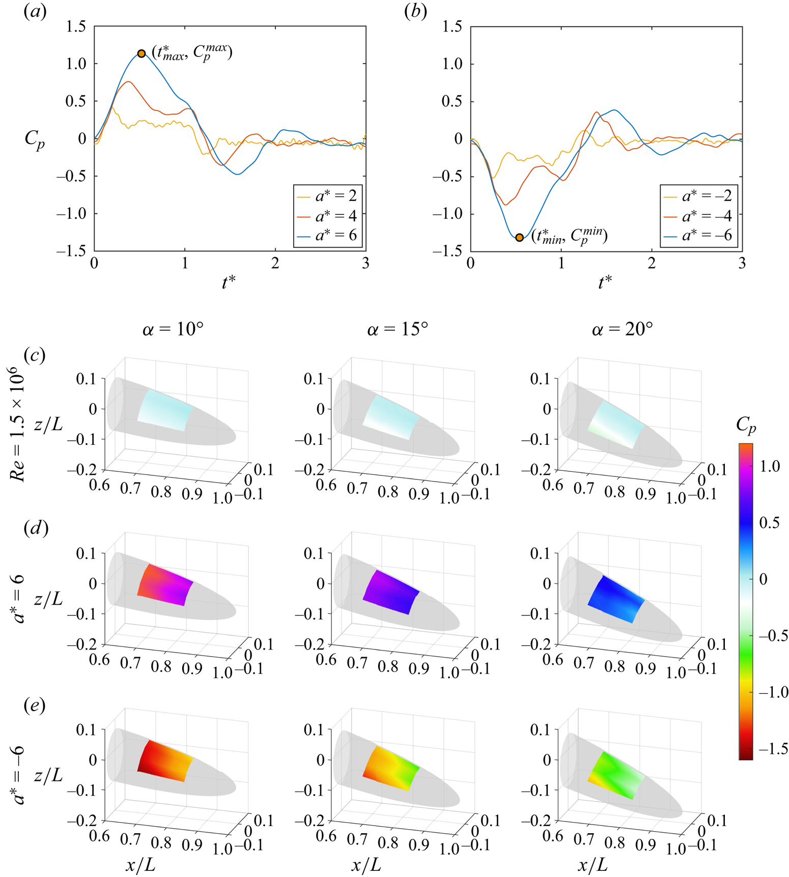
Figure 4. Ensemble-averaged pressure trends as a function of  $a^*$ and
  $\alpha$: (a,b) time evolution of the instantaneous pressure
  $C_p$ for a reference point (
 $x/L=0.7$,
  $\theta =0^\circ$) at
  $\alpha =10^\circ$ for various
  $a^*$; (c) steady surface pressure maps for
  $Re=1.5\times 10^6$; (d) surface pressure maps at time
  $t^*_{max}$ for
  $a^*=6$; and (e) surface pressure maps at time
  $t^*_{min}$ for
  $a^*=-6$. The incidence angle is indicated on the top of each column. Flow is from left to right.
In figure 4(c–e), the surface-pressure maps for the steady motion are compared with the pressure distributions at  $t^*_{max}$ (acceleration) and
  $t^*_{min}$ (deceleration) for
  $|a^*|=6$. The complete temporal evolution of acceleration (
 $a^*=6$) and deceleration (
 $a^*=-6$) can be seen in the supplementary movies (see supplementary Movies 1 and 2 available at https://doi.org/10.1017/jfm.2023.907). Each column corresponds to one incidence angle (
 $\alpha =10^\circ$,
  $15^\circ$ and
  $20^\circ$). The results for the steady condition with
  $Re = 1.5\times 10^6$ are first presented in figure 4(c). Although all
  $C_p$ values are relatively small, a circumferential pressure gradient is observable acting as the footprint of the cross-flow separation process. The circumferential pressure gradient is most significant at
  $\alpha =20^\circ$, corresponding to the strongest cross-flow separation driven both by streamwise APG and circumferential APG. For the accelerating case in figure 4(d), the
  $C_p$ values increase significantly in comparison to the steady condition. More importantly, for all
  $\alpha$, a strong streamwise FPG has been created in the longitudinal direction. This observation is in good agreement with theoretical approximations from the potential flow field around an accelerating sphere (Fernando et al. Reference Fernando, Marzanek, Bond and Rival2017). However, the significant flow separation on the back half of the prolate spheroid model influences the dynamics of the pressure coefficient (
 $C_p$) as well. Therefore, the acceleration magnitude and incidence angle have a direct impact on
  $C_p$. For the same acceleration (
 $a^*=6$), increasing
  $\alpha$ leads to a relative decrease of
  $C_p$. Larger
  $\alpha$ increases the size of the separated flow region and, thereby, decrease the influence of the acceleration on
  $C_p$. Furthermore, the circumferential pressure gradient, which is dominated under steady conditions, does not persist during the acceleration. This significant change in the pressure distribution is likely to lead to a movement of the separation line and to a change of the separated cross-flow wake (strong FPG).
The surface pressure distributions during deceleration are shown in figure 4(e) and opposite trends relative to the acceleration case were observed. A strong APG in the streamwise direction was established and the APG in the circumferential direction was increased.
3.2. Pressure gradients
The qualitative observations presented in § 3.1 are further quantified in this section, and the scaling of the pressure gradients is compared for different values of  $\alpha$ and
  $a^*$. We define two coefficients of streamwise and circumferential pressure gradients respectively as
 \begin{equation} \frac{\partial C_p}{\partial S_x}= \frac{C_p{(p_{x/L = 0.85})}-C_p{(p_{x/L =0.7})}}{dS_x/L} \end{equation}
and
 \begin{equation} \frac{\partial C_p}{\partial S_{\theta}}= \frac{C_p{(p_{\theta=0^\circ})}-C_p{(p_{\theta=90^\circ})}}{dS_{\theta}/L}, \end{equation}
where  $dS_x$ is the distance between two sensors along the longitudinal direction and
  $dS_{\theta }$ is the local circumferential distance at each cross-section. A higher absolute value of the coefficient indicates a stronger APG or FPG. The resulting pressure gradients are presented in figure 5. The black solid curve represents the steady condition of
  $Re = 1.5\times 10^6$ (used as a reference), the solid coloured lines depict accelerations and the dashed coloured curves present the pressure gradients during decelerations.

Figure 5. Trends in pressure gradients as a function of acceleration/deceleration magnitudes  $a^*$ and incidence angle
  $\alpha$: (a–c) for streamwise pressure gradient coefficient and (d–f) for spanwise pressure gradient coefficient. The incidence angle (
 $\alpha$) is indicated on the top of each column.
In figure 5(a–c), the streamwise pressure gradient ( $\partial C_p/\partial S_x$) is shown for various
  $\theta$ positions. For all
  $\theta$, acceleration causes the pressure-gradient field to be transformed from APG to FPG. Furthermore, the strength of the streamwise FPG is increased with increasing
  $a^*$, which is in good agreement with the theoretical predictions based on potential theory for an accelerating sphere (Fernando et al. Reference Fernando, Marzanek, Bond and Rival2017) and for an accelerating flat plate at incidence (Guo et al. Reference Guo, Zhang, Yasuda, Yang, Galipon and Rival2021), where the strength of the FPG was shown to be linearly dependent on the acceleration magnitude. In contrast, the pressure-gradient field is still covered by the streamwise APG for all decelerations and the strength of the APG increases also with increasing deceleration magnitude.
The distribution of  $\partial C_p/\partial S_{\theta }$ at
  $x/L\in \{ 0.70, 0.75, 0.80, 0.85 \}$ is presented in figure 5(d–f). For
  $Re = 1.5\times 10^6$, the circumferential APG strength increases from
  $\alpha =10^\circ$ to
  $\alpha =20^\circ$ due to the stronger cross-flow at a higher
  $\alpha$. As observed in § 3.1, the circumferential pressure gradient (
 $\partial C_p/\partial S_{\theta }$) is significantly reduced during acceleration. For
  $a^*=6$ at
  $x/L=0.85$, we even observe a weak circumferential FPG for all
  $\alpha$. While
  $\partial C_p/\partial S_{\theta }$ strongly depends on
  $\alpha$ for the steady reference case, the acceleration reduces
  $\partial C_p/\partial S_{\theta }$ to very small magnitudes, regardless of
  $\alpha$ or
  $a^*$. In contrast, the
  $\partial C_p/\partial S_{\theta }$ is further increased during decelerations, leading to strong circumferential APGs. The magnitude of
  $\partial C_p/\partial S_{\theta }$ is more affected by the deceleration for
  $\alpha =10^\circ$ than for the
  $\alpha =20^\circ$ case (compare figure 5d–f), where a large cross-flow separation already exists in the steady state.
Summarizing §§ 3.1 and 3.2, we conclude that the pressure-gradient field around an accelerating or decelerating spheroid is strongly influenced through axial acceleration. Not only is the magnitude of the pressure gradients influenced but furthermore, the gradient flips from APG to FPG in streamwise and circumferential directions. Therefore, we expect changes in the formation and subsequent evolution of the cross-flow structures as well.
3.3. Streamwise vorticity and velocity distributions
After observing the significant influence of the acceleration in § 3.2, we now discuss how the streamwise vorticity and velocity are influenced by acceleration. Here vorticity and velocity are normalized by the local instantaneous velocity ( $U_{inst}$) on each cross-section. The normalized (axial) vorticity is defined as
 \begin{equation} \omega_x^* = \frac{\omega_x L}{U_{inst}}. \end{equation}
Figure 6 presents the streamwise vorticity in the lab-fixed frame of reference and that  $u=U_{inst}$ would indicate that the fluid is moving at the same speed as the model. For sake of brevity, only the most extreme cases with largest acceleration (
 $a^*=6$) and deceleration (
 $a^*=-6$), at incidence angle
  $\alpha =20^\circ$, are shown in figure 6 and discussed in detail. For each case, three cross-sections (
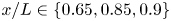 $x/L \in \{ 0.65, 0.85, 0.9 \}$; see figure 3) are examined to present the streamwise vorticity (
 $\omega _x^*$) and streamwise velocity (
 $u/U_{inst}$). The supplementary movie (see Movie 3) displays the complete evolution of vorticity on the rear section (
 $0.65\leq x/L \leq 0.90$). In figure 6, an orange diamond highlights the azimuthal position, where a significant deviation from the free-stream velocity is captured close to the model's surface. The orange diamond provides a visual indication for the extent of the cross-flow separation.

Figure 6. Streamwise vorticity and velocity for  $a^*=6$ and
  $a^*=-6$ at
  $\alpha =20^\circ$: (a–c) steady
  $Re=1.5\times 10^6$; (d–f)
  $A_{1.0L}$; (g–i)
  $A_{0.75L}$; (j–l)
  $A_{0.5L}$ and (m–o)
  $D_{1.0L}$. The size of the cross-flowseparation is highlighted by the orange diamonds on the streamwise velocity distributions. In the
  $A_{1.0L}$ and
  $A_{0.75L}$ cases, the separation point moves closer to the meridian centre of the model. In contrast, acceleration has no effect on the separation point in the
  $A_{0.5L}$ case. The point moves outwards in the
  $D_{1.0L}$ case.
Figure 6(a–c) presents results for the steady case as a reference. As discussed in a related study on steady wakes (Guo et al. Reference Guo, Kaiser and Rival2023), a helical vortex tube is formed at relatively small  $x/L$; see figure 6(a). Travelling downstream, the core of the vortex tube aligns with the mean flow direction, resulting in a high-velocity region away from the model, as highlighted in figure 6(b). To gather insights into the temporal evolution of the cross-flow during acceleration, we present cross-sections of all accelerations (
 $A_{1.0L}$,
  $A_{0.75L}$ and
  $A_{0.5L}$) and
  $t^*$ is indicated in the top right corner of each panel. Figure 6(d–f) shows
  $A_{1.0L}$ and thus the early evolution of the flow field directly after acceleration has begun. In figure 6(d), the flow has not yet adapted to the changing boundary conditions. However, downstream (figure 6e,f), the impact of the increased FPG is observable, and the original high-velocity region away from the model is already slightly suppressed. At the same time, the separation line has moved inwards indicating that the reduction in the circumferential APG (see § 3.2) directly impacts the location of the separation. The impact of the acceleration becomes even more apparent later on. Even though the acceleration is already complete in figure 6(h,i), most vorticity is concentrated close to the model surface and the momentum deficit in the wake is significantly reduced. As indicated by the dashed line, the helical vortex structures are closely attached to the spheroid at this time.
Figure 6(j–l) presents the post-acceleration evolution ( $A_{0.5L}$) and highlights how quickly the flow returns to steady state. The strong FPG reduces cross-flow separation and even reattaches the 3-D separated flows (Marzanek & Rival Reference Marzanek and Rival2019). However, in contrast with the hypothesis shown in figure 1(d), the flow does not fully reattach for the present kinematics. A sustained strong acceleration resulting in strong FPG at smaller incidence angles could still validate the hypothesis but goes beyond the scope of the present study. As shown in figure 6(k), the separation line moves outwards again at
  $t^*=1.68$, and vorticity and velocity fields already look very similar as in the steady state shown in figure 6(b). As such, the memory effect in the present flow relative to a sudden change of boundary conditions is significantly smaller when compared to previous studies on other model geometries such as by Kaiser et al. (Reference Kaiser, Kriegseis and Rival2020) and Marzanek & Rival (Reference Marzanek and Rival2019). Owing to the open separation on the elongated body of the prolate spheroid, the material volume of fluid that is directly affected by the acceleration quickly convects into the wake. In turn, the body acceleration quickly loses influence on the separated flow close to the prolate spheroid.
The  $D_{1.0L}$ case in figure 6(m–o) exhibits stronger flow separation due to the stronger APG in both streamwise and circumferential directions. The separation point moves away from the meridian, which is consistent with the hypothesis suggested in figure 1(e).
3.4. Circulation of streamwise vortices
The results up to this point show that dynamic motions have a significant influence on the resulting cross-flow structures. However, changes in the dynamic loads are often of primary interest in the context of flow separation on manoeuvring bodies. Prior studies have shown that the loads are closely connected to the separation size and strength, which can be further quantified by the circulation (Fu et al. Reference Fu, Shekarriz, Katz and Huang1994). In the current study, the circulation was obtained by integrating the streamwise vorticity over one side of the body (area  $A_H$ in figure 6c), such that normalized circulation can be defined as
 \begin{equation} \varGamma^* = \int_{A_H} \omega_x^* \,{\rm d}A_H. \end{equation}
In figure 7, the magnitude of  $\varGamma ^*$ is shown for the steady case (
 $Re = 1.5\times 10^6$),
  $A_{1.0L}$,
  $A_{0.75L}$,
  $A_{0.5L}$ and
  $D_{1.0L}$ all at
  $\alpha =20^\circ$. Figure 7(a) shows cases for acceleration
  $a^*=6$ and deceleration
  $a^*=-6$, while figure 7(b) represents
  $a^*=4$ and
  $a^*=-4$ since the streamwise FPG could be maintained for an extended period of time (see figure 4).

Figure 7. Circulation of streamwise vortices ( $\varGamma ^*$) at
  $\alpha =20^\circ$ with cross-sections (
 $x/L$): (a) for
  $a^*=6$ and
  $a^*=-6$; (b) for
  $a^*=4$ and
  $a^*=-4$. Only during acceleration (
 $A_{1.0L}$ case), acceleration has a great influence on the circulation. In contrast, deceleration works on strengthening flow separation.
The separated shear layer continues to feed vorticity into the cross-flow, which leads to an increase of  $\varGamma ^*$ with
  $x/L$. Thus, an increasing
  $\varGamma ^*$ indicates the growth process of the streamwise vortices along the body for all cases. The steady condition (
 $Re = 1.5\times 10^6$) is again shown as a reference in both panels. Note that if the response to the acceleration were to be instantaneous (quasi-steady), all lines would collapse since
  $\varGamma ^*$ is normalized by
  $U_{inst}$, see (3.4) and (3.5). However, when the
  $\varGamma ^*$ curve lies below the steady reference line, it suggests that less vorticity is shed into the cross-flow during acceleration. Varying growth rates for
  $A_{1.0L}$,
  $A_{0.75L}$,
  $A_{0.5L}$ and
  $D_{1.0L}$ are observed, and will be discussed below to explain the effects of acceleration or deceleration on vortex formation.
We start the discussion with  $A_{1.0L}$. The
  $\varGamma ^*_{A_{1.0L}}$ curve begins to deviate from the steady reference for
  $x/L>0.7$, indicating a lag in the flow to the acceleration that started at
  $x/L= 0.6$. In the following, the difference between
  $A_{1.0L}$ and the steady reference increases as highlighted by
  $\Delta \varGamma ^*$ in figure 7(a). This increasing deviation shows how the helical vortices do not directly adapt to the instantaneous velocity. Consistent with the
  $A_{1.0L}$ result, the circulation from
  $A_{0.75L}$ starts with smaller values than the steady reference case but approaches the steady result later. Finally, for
  $A_{0.5L}$, the sPIV measurement takes place after the acceleration is completed. It is apparent that
  $\varGamma ^*$ is quite similar to the steady curve, reconfirming the short-lived memory effect for the open cross-flow as mentioned in § 3.3. The deceleration case is represented by a dashed line in figure 7(a) and shows much higher normalized circulation values, indicating a stronger cross-flow separation than the steady or accelerated cases. This observation is in good agreement with the instantaneous vorticity fields shown in figure 6(m–o).
Finally, the evolution of  $\varGamma ^*$ at
  $a^*=4$ and
  $a^*=-4$ is shown in figure 7(b). The same trends can be observed as in figure 7(a). However, the gap
  $\Delta \varGamma ^*$ is smaller than that for
  $a^*=6$. The
  $\varGamma ^*$ curve for the
  $A_{0.75L}$ case is relatively high when compared with the steady result at
  $0.7 \leq x/L \leq 0.8$, which is attributed to the stronger shear layer, as shown in figure 6(h).
4. Conclusions
A series of experiments to investigate the dynamic separation on an accelerating and decelerating prolate spheroid have been conducted. The instantaneous surface pressure, as a function of acceleration strength ( $a^*$) and incidence angle (
 $\alpha$), has been collected, and the 3-D flow separation about the prolate spheroid was measured using scanning sPIV, from which the moving separation line, the streamwise momentum deficit, the streamwise vorticity and eventually the circulation have all been extracted.
The main findings in the current study are summarized as follows.
(1) The pressure gradient on the prolate spheroid responds rapidly to axial acceleration and deceleration. During acceleration, the character of the streamwise pressure gradient transforms from adverse to favourable. Furthermore, the strength of the streamwise FPG increases with increasing acceleration magnitude. This phenomenon is stronger for small
 $\alpha$. At the same time, the acceleration removes the circumferential pressure gradients, which are prominent during steady motion. In contrast, for a decelerating prolate spheroid, the streamwise and the circumferential adverse pressure gradients are both amplified.
(2) The separation line on the prolate spheroid surface moves as a result of the rapid change in streamwise velocity. The separation line moves closer to the model meridian centre during acceleration as a result of the vanishing circumferential APG, while moving outwards during deceleration due to a stronger APG along both streamwise and circumferential directions.
(3) In addition to the moving separation line, an axial acceleration also leads to a change of the flow structures in the separated cross-flow. The helical vortex structure remains close to the model and does not align with the mean-flow direction as is observed for the steady case. As such, a region of concentrated vorticity was observed close to the body, while the momentum deficit in the wake is reduced. In contrast, for axial deceleration, the wake remains aligned with the mean-flow direction. However, more vorticity is shed, leading to an increase in streamwise circulation.
(4) While the surface pressures react instantaneously to acceleration, the observed flow fields respond with a small delay. This lag is in good agreement with earlier studies with hysteresis in unsteady turbulent separation (Ambrogi, Piomelli & Rival Reference Ambrogi, Piomelli and Rival2022). Furthermore, the separation line remains at its unaltered position even shortly after the acceleration is completed, indicating a weak memory effect in the cross-flow. However, the cross-flow recovers quickly to the steady state and the separation line moves back to its original location.

Despite the insights gathered in the present manuscript, several open questions remain. For instance, would sustained accelerations at smaller incidence angles reattach the separated flow? Future work could also decouple the effects of the pressure gradient and curvature on the formation of 3-D cross-flow separation by systematically varying the model geometry.
Supplementary movies
Supplementary movies are available at https://doi.org/10.1017/jfm.2023.907.
Acknowledgements
The authors would like to thank Wenchao Yang and Dashuai Chen for assistance with the initial experimental set-up, as well as JiaCheng Hu and Adnan EI Makdah in the same research group for their fruitful input.
Funding
The research was supported by DER's NSERC Discovery grant.
Declaration of interests
The authors report no conflict of interest.
Author contributions
All authors, conceptualization and methodology; P.G. and F.K., experimental execution, software, visualization and writing of the original draft; D.E.R., acquisition of funding, supervision, reviewing and editing.
Appendix
The cases with the largest acceleration ( $a^* = 6$) and deceleration (
 $a^* = -6$) at a milder incidence angle
  $\alpha =10^\circ$ are compared in figure 8. Identical to figure 6, three cross-sections (
 $x/L \in \{ 0.65, 0.85, 0.9 \}$) are chosen to present the streamwise vorticity (
 $\omega _x^*$), streamwise velocity (
 $u/U_{inst}$) and the trend of the moving separation point. Figure 8(a–c) shows steady results as a reference. Compared with the largest incidence angle
  $\alpha =20^\circ$, a much smaller cross-flow separation is observed above the model surface. For temporal evolution of the cross-flow separation during the acceleration (
 $A_{1.0L}$, figure 8d–f), the impact of the increased FPG can be observed through the suppressed high-velocity region. The inward movement of the separation line also indicates the reduction in the circumferential APG, showing the same trend as the observation in figure 6(d–f). When the acceleration is complete, as seen in figure 8(g–i), the vorticity is more concentrated and the helical vortex structures more closely adhere to the model surface, corresponding to the observation in figure 6(h–i). Figure 8(j–l) represents deceleration conditions (
 $D_{1.0L}$) and shows enhanced flow separation due to a stronger APG in both the streamwise and circumferential directions. The trend in the separation point movement is also consistent at the largest incidence angle
  $\alpha =20^\circ$. However, due to the small cross-flow separation, whether the separated flow re-attaches on the model surface under these current accelerations cannot be confirmed.
Figure 8. Streamwise vorticity and velocity for  $a^*=6$ and
  $a^*=-6$ at
  $\alpha =10^\circ$: (a–c) steady
  $Re=1.5\times 10^6$; (d–f)
  $A_{1.0L}$; (g–i)
  $A_{0.5L}$ and (j–l)
  $D_{1.0L}$. The location of the separation point is marked by the orange diamonds on the streamwise velocity distributions.


 Open access