


1. Introduction
Droplet impact onto wetted surfaces is of pertinence to many technical and environmental applications such as soil erosion, internal combustion engines, icing on plane wings and spray coating technologies. Immediately after the impact, the droplet expands radially along the surface. If the impact kinetic energy is sufficiently high to overcome energy losses arising from deformation and viscous effects, an upward growing crown is generated with detachment of secondary droplets (splashing regime). Different theoretical models have been proposed in the literature to describe this process, which can be conceptually divided into three phases. Phase 1 focuses on the early stage of the impact dynamics, as shown schematically in figure 1(a). Specifically, it describes the initial deformation of the droplet during impact and the spreading of the contact line up to a dimensionless time of  $\tau = t U_0 / D_0 = {O}(10^{-1})$. Here, $U_0$ and $D_0$ denote the velocity and diameter of the impacting droplet, respectively. Philippi, Lagrée & Antkowiak (Reference Philippi, Lagrée and Antkowiak2016) performed numerical simulations of this phase for a single droplet impact onto a dry wall. They found that the wet footprint of the droplet dictates the size of the impact-induced perturbed flow. The latter exhibits an inviscid stagnation point flow structure and admits a self-similar solution, where both the pressure and velocity variables depend solely on the self-similar variables $(r / \sqrt {t}, z / \sqrt {t})$ both in the outer region and in the boundary layer. Here, the variables $r$ and $z$ denote the radial and vertical coordinates, respectively. Moreover, they found that the contact line (CL) propagates in time according to the following relation: $r_{CL}=\sqrt {3 D_0 U_0 t/2}=D_0 \sqrt {3 \tau /2}$. For droplet impact on a wetted wall, Yarin & Weiss (Reference Yarin and Weiss1995) demonstrated that, within the wet footprint of the droplet, momentum is also transferred to the wall film. Moreover, they modelled the resulting decay of the film height with time ( $h_{F}(t)$). A detailed description of their model for the droplet induced flow is presented in § 2, owing to its relevance for our analytical solution. Phase 2 is seamlessly connected to Phase 1 and focuses on the modelling of the crown formation. As shown by Philippi et al. (Reference Philippi, Lagrée and Antkowiak2016), the liquid lamella emerges from the contact line and follows closely its trajectory during the early stage. Yarin & Weiss (Reference Yarin and Weiss1995) showed theoretically that the emergence of a crown-like lamella corresponds to the onset of a velocity (kinematic) discontinuity (KD) with a mass sink (liquid outflow) at its front, owing to the incompressibility of the liquid layer, as shown in figure 1(b). Phase 3 focuses on the late stage of the droplet impact process and describes the propagation of the KD. For this phase, Yarin & Weiss (Reference Yarin and Weiss1995) proposed the following model for describing the crown propagation in the case of droplet impact onto a wet substrate. Specifically, the radius at the foot of the KD $R_{KD}$ (see figure 1b) is modelled as $\bar {R}_{KD} = R_{KD}/D_0 = \beta _{YW} \sqrt {\tau - \tau _0}$. Here, $\beta _{YW} = (2/(3\delta))^{1/4}$ is an empirical constant, obtained by fitting the experiments of Levin & Hobbs (Reference Levin and Hobbs1971) for $\delta =0.17$, with $\delta = h_0 /D_0$ representing the initial dimensionless film thickness. The constant $\beta _{YW}$ essentially describes the effect of wall-film inertia on the rate of crown propagation. Over the years, several correlations have been proposed to improve the agreement with experiments by modifying the value of the constant $\beta _{YW}$ with varying Weber and Reynolds numbers. In all cases, the following functional dependence for the radius of the KD was maintained: $\bar {R}_{KD} = \beta \tau ^{n}$. An overview of the different correlations can be found in table 1.

Figure 1. Schematics of drop impact and formation of the KD: (a) Phase 1, early stage of droplet induced flow; (b) Phase 2, formation of the KD. The subscripts ‘ $res_D$’ and ‘ $F$’ refer to the residual droplet and wall-film liquid layers, respectively.
Table 1. Overview of empirical correlations  $\bar {R}_{KD} = \beta \tau ^{n}$ describing the propagation of the crown, i.e. the evolution of the radius of the KD.

Recently, Gao & Li (Reference Gao and Li2015) proposed a unified framework to integrate and compare competing modelling approaches, according to  $\bar {R}_{KD} = (\beta _{YW} \sqrt {\lambda }) \sqrt {\tau } + C_0$. Indicating with $m_{D}$ the mass of the droplet, the empirical parameter $\lambda = m_{D} u_{im}/m_{D} U_0 = 0.26 Re_D^{0.05} / (We_D^{0.07} \delta ^{0.34})$ represents the reduction in transmitted momentum arising from impact losses. In this respect, $u_{im}$ can be interpreted as the momentum per unit mass, i.e. specific momentum. Here, the Reynolds ( $Re_D = U_0 D_0 / \nu$) and Weber ( $We_D = \rho U^{2}_0 D_0 / \sigma$) numbers are defined on the basis of the physical properties of the impacting liquid droplet, where $\nu$, $\rho$ and $\sigma$ denote the kinematic viscosity, density and surface tension, respectively. Consequently, the characteristic inertial time for crown propagation is now defined as $t_{cit}=D_0/(\lambda U_0)$. The parameter $\lambda$ was included in the definition of the square-root pre-factor ( $\beta _{GL} = \beta _{YW} \sqrt {\lambda }$) to maintain the same definition of the dimensionless time $\tau = U_0 t / D_0$. The initial offset $C_0(\delta )$ is only a function of $\delta$ and is analytically derived under the assumption that the droplet volume is completely transformed into a liquid cylinder of height $h_{0}$. The physical insight of Gao & Li (Reference Gao and Li2015) is that the temporal evolution of the crown (KD) will follow the same curve only when the combined effect of deformation, viscous and inertial forces leads to the same value of the constant $\beta _{GL}$. This can be clearly seen in figure 2(a), where the solid black and red curves exhibit a very similar trend despite the large difference in Weber and Reynolds numbers. Moreover, it shows that the Gao & Li model is capable to reproduce the correlations of Cossali et al. and Rieber & Frohn (correlations No. 3 and 4 in table 1, respectively), thanks to the introduction of the $\sqrt {\lambda }$-factor in the original Yarin & Weiss model (see table 1). Figure 2(a) also shows that the initialisation procedure to determine $C_{0}(\delta )$ looses accuracy with increasing film thickness $\delta$, as discussed in detail in § 2.6. Figure 2(b) extends the comparison with experiments to a longer time scale and confirms the previous statement on the inaccuracy of the $C_{0}$-initialisation with increasing $\delta$. Moreover, in the late stage of Phase 3, the experimental data exhibit a systematic deviation from the postulated $\sqrt {t}$-dependence. Two primary mechanisms may be responsible for this deviation: (1) crown contraction owing to the restoring action of surface tension; (2) attenuation of the crown speed owing to boundary layer effects.

Figure 2. Empirical correlations for the temporal evolution of the crown (KD). (a) Comparison among the correlations of Rieber & Frohn (Reference Rieber and Frohn1999) (RF), Cossali et al. (Reference Cossali, Marengo, Coghe and Zhdanov2004) (Cos), Yarin & Weiss (Reference Yarin and Weiss1995) (YW) and Gao & Li (Reference Gao and Li2015) (GL). All correlations are listed in table 1. (b) Comparison of experimental data (exp. No. 5,7) with theoretical models. Detailed test conditions can be found in table 3 in Appendix B.
In this work, we will mainly investigate the relevance of momentum losses during crown propagation. This requires an accurate estimation of the strain rate in the boundary layer, which depends not only on the fluid viscosity, but also on the thinning rate of the liquid layer. For this purpose, we propose an extension of the Yarin & Weiss analytical solution by incorporating explicitly the boundary layer profile in the evolution of the radial velocity component both for the flow field within the impact zone and for the KD. This is shown schematically in the inset of figure 1(b). The rationale for this choice is the following. In contrast to all models listed in table 1, the Yarin & Weiss approach is the only one that provides a comprehensive analytical solution for the two-dimensional flow field, for the wall-film decay and for the position of the KD. As shown in § 3, the inclusion of momentum losses allows an accurate prediction of the KD-spreading rate and enables a smooth transition from the inertia-driven to the shear-controlled regime of crown propagation.
2. Modelling approach
This section describes in detail the modelling approach for Phase 3. The proposed solution encompasses the inclusion of boundary layer effects both in the propagation of the KD and in the flow field within the impact zone, the estimation of the thinning rate of the liquid layer and its residual thickness. In the process, we also propose an alternative method to initialise the solution for the KD propagation. This leads indirectly to an estimation of the total length of the impact zone ( $L_{im}$) and of the KD formation time ( $\tau _{ini}$) for impact events on both dry and wetted walls. For ease of reading, the description of the modelling approach has been subdivided into several sub-sections, even though all modelling aspects are part of a unified approach.
2.1. Solution for the KD
The starting point of the theoretical model of Yarin & Weiss (Reference Yarin and Weiss1995) was to solve the one-dimensional, axisymmetric momentum equation in conservative form (i.e. negligible viscous losses). This equation admits velocity discontinuities as a solution, when the initial velocity distribution in the liquid layer ( $u = F(\zeta )$) has a finite large value in the impact zone and then rapidly drops to zero outside the wet footprint of the droplet, as shown in the pictorial illustration in figure 3(a). The variable $\zeta$ denotes the radial coordinate in the impact zone. In contrast to the original work of Yarin & Weiss (Reference Yarin and Weiss1995), here the origin of the coordinate axis is set at the centre of the impact zone, yielding the following coordinate transformation: $\zeta = \zeta ' + 0.5 L_{im}$. For a small value of $\zeta$, Yarin & Weiss (Reference Yarin and Weiss1995) assumed that the initial velocity distribution in the liquid film can be approximated as $F(\zeta ) = B \zeta$, with $B$ being a positive constant. Consistently with the previous assumption, Yarin & Weiss further assumed the maximum extent of the impact zone $L_{im}$ to be proportional to $D_{0}$, yielding $L_{im}=\alpha D_{0}$ with $\alpha >0$. Following Whitham (Reference Whitham1974), the equations describing the position and velocity of the KD in the asymptotic regime (large $t$, alias Phase 3) read as
 \begin{equation} A = \int_{{-}0.5L_{im}}^{0.5L_{im}} F\left(\zeta' + \frac{L_{im}}{2} \right) {\rm d}\zeta', \quad u_{KD} = \frac{1}{2} \sqrt{\frac{2A}{t}}, \quad R_{KD}(t) = \sqrt{2At}. \end{equation}
The parameter  $A$ is defined as the integral of the initial velocity distribution $F(\zeta )$ within the impact zone. It represents the total amount of kinetic energy transferred by the impacting droplet to the KD. To estimate the value of the parameter $A$, it is therefore necessary to relate the initial velocity distribution $F(\zeta ) = B \zeta$ to the impact conditions. In this work, we propose to estimate the constant $B=a_0 = \lambda U_0 / D_0$, so that it represents the specific momentum transferred per unit length from the impacting droplet to the liquid layer. Substituting this value in (2.1a–c) yields
 \begin{equation} A=\int_{{-}0.5 \alpha D_0}^{0.5 \alpha D_0} a_o \left (\zeta' + \frac{\alpha D_0}{2} \right) {\rm d}\zeta' = a_0 \frac{\alpha^{2} D_0^{2}}{2}. \end{equation}
Consequently, the velocity and location of the KD can be modelled as
 $$\begin{gather} \bar{u}_{KD} = \frac{u_{KD}}{U_0} = \frac{\alpha \sqrt{\lambda}}{2\sqrt{\tau}}, \end{gather}$$
 $$\begin{gather}\bar{R}_{KD} = \alpha \sqrt{\lambda} \sqrt{\tau}. \end{gather}$$
Equation (2.4) shows that the semi-empirical correlation for  $\bar {R}_{KD}$ of Gao & Li (Reference Gao and Li2015) can be recovered by setting $\alpha =\beta _{YW} = (2/(3\delta))^{1/4}$ (see table 1, correlation No. 2). Alternatively, if we neglect impact losses (i.e. $\lambda =1$), the formula of Yarin & Weiss (Reference Yarin and Weiss1995) is reobtained (correlation No. 1 in table 1). This finding not only confirms the validity of the proposed estimation for the constant $B$, but yields also a measure for the extent of the impact zone. In non-dimensional terms, the variation of $L_{im}/D_0 = \alpha$ is plotted in figure 3(b) as a function of $\delta$. As can be seen, the impact length decreases monotonically with the wall-film thickness and tends to the droplet diameter $D_0$ with increasing $\delta$. This means that with increasing the wall-film inertia, the size of the liquid volume displaced by the impacting droplet to form the KD will decrease. In this context, it is important to point out that this trend is based on the functional dependence proposed for the empirical constant $\beta _{YW}$ with $\delta$. The latter was validated against the experiments of Levin & Hobbs (Reference Levin and Hobbs1971) for $\delta = 0.17$. Note that the uncertainty in the estimation of the non-dimensional wall-film thickness (nominally $\delta = 0.17$) for these experiments cannot be ascertained. Moreover, an anomaly is observed for $\delta \leqslant 0.1$, where the predictions for $L_{im}$ are even larger than the maximum distance covered by the KD over the entire duration of a splashing event, as shown in § 3. A possible explanation is to assume that, for $\delta \leqslant 0.1$, the wall film is almost completely removed from the impact zone. Consequently, the propagation of the contact line/KD is mainly limited by friction losses at the wall rather than by wall-film inertia. For droplet impact on dry walls, Philippi et al. (Reference Philippi, Lagrée and Antkowiak2016) found for the contact line: $\bar {r}_{CL} = \sqrt {3/2} \sqrt {\tau }$ (see also table 1, correlation No. 9). The coefficient $\beta _{Ph} = \sqrt {3/2}$ is also plotted in figure 3(b) for comparison. As can be seen, friction effects limit the propagation of the KD more effectively than wall-film inertia effects. For the estimation of the total extent of the impact zone, we decided therefore to adopt $\beta _{Ph}$ for $\delta \leqslant 0.2$ and then $\beta _{YW}$ for $\delta > 0.2$. In support of this choice, we refer to the overview shown in table 1. As can be seen, very few experiments or simulations have been performed for $\delta \leqslant 0.1$ for which the value of the parameter $\beta$ was specified. The only noteworthy exception is provided by the simulations of Rieber & Frohn (Reference Rieber and Frohn1999), who found a value of $\beta \approx 1.1$ for $\delta \approx 0.12$, which is very close to the constant $\beta _{Ph} = \sqrt {3/2}$ for impact on a dry wall (Philippi et al. Reference Philippi, Lagrée and Antkowiak2016). Moreover, with reference to figure 3(b), one can see that for $\delta = 0.2$, the difference between $\beta _{Ph}$ and $\beta _{YW}$ becomes minor, thus justifying the choice of 0.2 as the transition value. The validity of this approximation for estimating the total extent of the impact zone $L_{im}$ is verified in § 3 through comparison with experimental data.

Figure 3. Extent of the impact zone: (a) schematic of its evolution; (b) non-dimensional maximum length of impact zone  $L_{im}/D_0$ as a function of non-dimensional film thickness $\delta$.
2.2. Flow field solution within the impact zone
For modelling the flow field within the impact zone, the momentum balance equation in the radial direction, written in cylindrical coordinates for an axisymmetric flow, is considered. Neglecting the body force and indicating with  $u$ and $w$ the velocity component in the radial and vertical directions, it follows
 \begin{equation} \frac{\partial u}{\partial t} + u \frac{\partial u}{\partial r} + w \frac{\partial u}{\partial z} = \nu \left [ \frac{\partial u}{\partial r} \left( \frac{1}{r} \frac{\partial (ur)}{\partial r} \right ) + \frac{\partial^{2} u}{\partial z^{2}}\right ] - \frac{1}{\rho} \frac{\partial p}{\partial r} . \end{equation}
As an outer flow solution for the inviscid flow, the potential flow solution of Yarin & Weiss (Reference Yarin and Weiss1995) is adopted with  $B=a_0$. This yields the following expressions for the induced flow velocity within the impact zone, valid for the asymptotic regime:
 \begin{equation} u(t)= \left( \frac{a_0}{1+a_0 t} \right ) r = a(t) \, r, \quad w(t)={-} 2a(t) \, z. \end{equation}
These findings show that the impacting droplet transfers momentum to the liquid layer both radially and vertically. In particular, the outer flow induced in the radial direction has the functional dependence of a stagnation point flow with decaying strength  $a(t)$. Moreover, the decay in the wall-film height was modelled as follows (Yarin & Weiss Reference Yarin and Weiss1995):
 \begin{equation} h_{F}(t) =\frac{h_0}{(1+ a_0 t)^{2}}. \end{equation}
Note that (2.7) can also be obtained by directly integrating the outer momentum equation in the  $z$-direction: $w=\partial z/ \partial t = -2a(t)z$ in the interval [0, $t$] and [ $h_0$, $h_{F}(t)$].
The boundary layer solution can be obtained by reducing the Navier–Stokes equations to an ordinary differential equation. This can be achieved by eliminating the time dependence through the coordinate transformation proposed by Roisman (Reference Roisman2009):
 \begin{equation} \xi = \sqrt{\frac{a(t)}{\nu t}}z, \quad g(\xi) = \frac{\psi \sqrt{t}}{r^{2} \sqrt{\nu \, a(t)}}, \end{equation}
where  $\psi$ denotes the stream function. The velocity components are then transformed as
 \begin{equation} u = \frac{1}{r} \frac{\partial \psi}{\partial z} = \frac{a(t) r}{t} g' \left( \xi \right ) \quad w ={-} \frac{1}{r} \frac{\partial \psi}{\partial r} ={-}2 \sqrt{\frac{\nu \, a(t)}{t}} g \left( \xi \right ). \end{equation}
With this transformation, the unsteady term is subsequently expressed as
 \begin{equation} \frac{\partial u}{\partial t} = \frac{\partial }{\partial t} \left[ \frac{a(t) \, r}{t} g' \left( \xi \right ) \right ] ={-} \frac{a(t) \, r}{t^{2}} \left ( \frac{\xi}{2} g'' + g' \right ) \left [1 + \overbrace{\frac{a_o \, t}{(1 + a_0 \, t)}}^{\varepsilon(t)} \right]. \end{equation}
The function  $\varepsilon (t)$ represents an additional contribution owing to the temporal variation of $a(t)$ and varies between 0 (for $t=0$) and 1 (for $t \rightarrow \infty$) (see derivation in Appendix A). In the transformed coordinate (Drazin & Riley Reference Drazin and Riley2007), the radial pressure gradient for an unsteady, viscous, axisymmetric stagnation-point flow can be expressed as
 \begin{equation} \frac{p - p_0}{\rho} ={-} \frac{1}{2} [a(t)]^{2} r^{2} \left ( \frac{g'}{t} \right )^{2} - 2 \, \nu \, a(t) \left ( \frac{g^{2}}{t^{2}} + \frac{g'}{\sqrt{t}} \right ) . \end{equation}
For the radial derivative we then obtain
 \begin{equation} \frac{1}{\rho} \frac{\partial p}{\partial r} ={-} \frac{[a(t)]^{2} \, r}{t^{2}} g'. \end{equation}
Because the pressure is transmitted integrally through the boundary layer, (2.12) can be evaluated in the free stream, where  $g'=1$. Calculating all other derivatives in a similar manner and substituting these expressions into (2.5) yields
 \begin{equation} g''' + 2 g g'' - g'^{2} + 1 + \underbrace{\frac{[1+\varepsilon(t)]}{a(t)} \left ( \frac{1}{2}\xi g'' + g' \right )}_{\mathrm{unsteady \ term}}= 0, \end{equation}
with the boundary conditions
 \begin{equation} \xi = 0: \quad g = 0, \ g' = 0; \quad \xi \rightarrow \infty: \quad g' = 1. \end{equation}
In the transformed coordinate system (2.13), the order of magnitude of the unsteady term is basically weighted by the factor  $1/ a(t)$, being $0 \leqslant \varepsilon (t) \leqslant 1$. The temporal variation of $a(t)$, as derived by Yarin & Weiss (Reference Yarin and Weiss1995) (see (2.6a,b)), is shown in figure 4(a) for selected experiments. For the typical duration of a splashing experiment ( $t_{max} \approx 30$ ms), $a(t)$ never attains a value lower than $30\ {\rm s}^{-1}$. Hence, irrespective of the value of the function $\varepsilon (t)$, the unsteady term is at least one or two order of magnitudes smaller than the convective or diffusive terms. This statement is further corroborated by performing a parametric analysis of the unsteady pre-factor. After simple algebra, the latter can be re-written as $[1+\varepsilon (t)]/a(t)=({1}/{a_0})+2t$. Its temporal evolution is shown in figure 4(b) for characteristic values of the parameter $a_0$, which, to a large extent, controls the order of magnitude of the unsteady term. For the present splashing experiments, the parameter $a_0$ is always comprised in the range $460 < a_0 < 1060\ {\rm s}^{-1}$ (see Appendix B), thus confirming the negligibility of the unsteady term in the transformed coordinate system, i.e. in (2.13). This feature has important implications on the characteristics of the solution for the velocity profile $g'(\xi )$. Indeed, by solving the third-order ordinary differential equation (ODE) for different fixed values of the parameter $a(t)$ and $\varepsilon (t)$, we found that all solutions merge into a single curve for $a(t) \geqslant 100\ {\rm s}^{-1}$, while minor deviations appear only for $a(t) = 10\ {\rm s}^{-1}$, as shown in figure 5(a,b). The advantage of this finding is mainly from a computational point of view. Indeed, as shown in § 3, the estimation of momentum losses during crown propagation can be made with reasonable accuracy by employing the solution of (2.13), obtained at a constant fixed value for the parameter $a$ (e.g. $a_0$), without the need of employing a time consuming iterative approach. In summary, thanks to the short duration of a splashing event ( $t_{max} \approx 30$ ms), our analysis shows that a self-similar solution can also be obtained for the boundary layer of an unsteady stagnation point flow with decaying strength $a(t)$. The present self-similar solution in the variables $[r \sqrt {a(t) /(\nu t)}, z \sqrt {a(t) / (\nu t)} ]$ represents a straightforward generalisation of the self-similar, inviscid stagnation point flow solution in the variables $(r / \sqrt {t}, z / \sqrt {t})$ established by Philippi et al. (Reference Philippi, Lagrée and Antkowiak2016).

Figure 4. Evaluation of unsteady term: (a) temporal dependence of the function  $a(t)=a_0/(1+a_0 t)$ on the input parameter $a_0 = \lambda U_0 / D_0$ for selected experiments (No. 1,2 (n-hexadecane), 9 (hyspin), 15,17 (B3), 18,20 (B10) and 21,23 (B50), see tables in Appendix B) covering a range of $460< a_0<1060\ {\rm s}^{-1}$; (b) dependence of the unsteady term's pre-factor $({1+\varepsilon (t)})/{a(t)}=({1}/{a_0})+2t$ of (2.13) on the input parameter $a_0$.

Figure 5. Overview of the different solutions for the unsteady stagnation point flow in the transformed coordinate system: (a)  $\varepsilon (t)$ dependence; (b) $a$ dependence.
2.3. Estimation of momentum losses
The momentum losses are determined solely for the spreading phase of the crown (Phase 3), thanks to the availability of an analytical solution for the outer flow for both the KD and the flow field within the impact zone. For this purpose, the first step is to model the decay of the liquid layer  $h_{tot}(t)$ at the foot of the crown (see figure 1b), defined as $h_{tot}(t) = h_{res_D} + h_F(t)$. The subscripts ‘ $res_D$’ and ‘ $F$’ refer to the residual droplet and wall-film liquid layers, respectively. The estimation of the liquid layer's decay rate as well as of the residual film thickness is discussed in § 2.4. Hereafter, we describe the approach adopted in this work to estimate the momentum losses. The latter can be evaluated by introducing a profile-averaged non-dimensional velocity according to
 \begin{equation} \bar{g}' = \frac{{u}^{v}}{u_{\infty}} = \frac{1}{\xi_{max}} \int_{0}^{\xi_{max}} g' \,{\rm d}\xi =\frac{1}{\xi_{max}} g(\xi_{max}), \quad \xi_{max} = \sqrt{\frac{a(t)}{\nu t}} h_{tot}(t). \end{equation}
Here  $\xi _{max}$ represents the total scaled height of the liquid layer in the transformed coordinate system. The definite integral in (2.15a,b) yields no integration constant, because $g(\xi )$ crosses the origin. Equation (2.15a,b) essentially estimates the momentum carried by the moving lamella by calculating the total area of the velocity profile and dividing it by the non-dimensional height of the liquid layer. Its physical meaning is schematically illustrated in figure 6(a). The momentum losses are represented by the red area. In the inviscid approximation (e.g. Gao & Li Reference Gao and Li2015), the velocity is constant along the wall film (grey rectangular area). Hence, (2.15a,b) yields ${u}^{v}(t)=u_{\infty }(t)$. If we now incorporate a boundary layer flow close to the wall, (2.15a,b) measures the average momentum carried by the lamella ${u}^{v}(t)$, deprived of momentum losses, as a fraction of $u_{\infty }(t)$. Note that $\bar {g}'(\xi _{max})$ is not constant in time, as it is implicitly a function of the total height $h_{tot}(t)$. Hence, even though the shape of the self-similar solution $g(\xi )$ does not change in time, the profile-averaged non-dimensional velocity $\bar {g}'(\xi _{max})$ will vary between approximately one (when $h_{tot} \gg h_{res}$) and an asymptotic value (when $h_{tot} \rightarrow h_{res}$). Owing to the self-similarity of the boundary layer solution, the analytical function $\bar {g}'(\xi _{max})$ can be employed to estimate the attenuated flow velocity at any radial location between the impact point and the KD. As a first step, the averaged velocity is transformed back to the physical coordinate system according to
 \begin{equation} \frac{{u}^{v}(t)}{u_{\infty}} = \lambda_1(t) = \frac{1}{\sqrt{\dfrac{a(t)}{\nu t}} h_{tot}(t)} g \left [ \sqrt{\frac{a(t)}{\nu t}} h_{tot}(t) \right ]. \end{equation}
In this work, we are only interested in determining the crown's speed. Hence,  $u_{\infty }$ denotes the velocity outside the boundary layer as determined by potential theory (see (2.3)) and $\lambda _1(t)$ represents the loss in momentum arising from viscous forces. It follows
 $$\begin{gather} \bar{u}_{KD}^{v} = \lambda_1 \frac{{u}_{KD}}{U_0} = \frac{\alpha \lambda_1 \sqrt{\lambda}}{2\sqrt{\tau}}, \end{gather}$$
 $$\begin{gather}\quad \bar{R}_{KD} = \alpha \lambda_1 \sqrt{\lambda} \sqrt{\tau - \tau_{ini}} + \bar{R}_{KD,ini}. \end{gather}$$
Direct integration of the velocity  $\bar {u}_{KD}^{v}(\tau )$ yields the function $\bar {R}_{KD}(\tau )$, where [ $\tau _{ini},\bar {R}_{KD,ini}$] represent the starting values of a fully formed crown at the end of the impact phase. Based on the discussion presented in the §§ 1 and 2.1, (2.17) and (2.18) include all the recent literature findings. Specifically, the impact losses are incorporated through the factor $\sqrt {\lambda }$, in compliance with the analysis of Gao & Li (Reference Gao and Li2015). The pre-factor $\alpha$ is modelled as $\alpha = \beta _{Ph}$ for $\delta \leqslant 0.2$ to take into account that the extent of the impact zone is mainly limited by friction losses, in compliance with the analysis of Philippi et al. (Reference Philippi, Lagrée and Antkowiak2016). Instead, for $\delta > 0.2$, we set $\alpha = \beta _{YW}$ to take into account that the extent of the impact zone is mainly determined by the wall-film inertia, in compliance with the findings of Yarin & Weiss (Reference Yarin and Weiss1995). The advantage of this approach is that it provides a unified solution for droplet impact on both dry and wetted walls. The validity of this choice is verified in § 3.

Figure 6. (a) Graphic visualisation of momentum losses. The grey area represents the momentum carried by the lamella, deprived of momentum losses (red striped area). (b) Dimensionless residual thickness of the droplet liquid layer for impact on dry and wetted walls. For impacts on dry walls, the comparison between experimental and numerical correlations shows an excellent agreement.
2.4. Estimation of the liquid layer's evolution
Equation (2.16) shows that modelling the temporal evolution of the liquid layer  $h_{tot}(t)$ is a key requisite for determining the viscous losses. In this work, we assume that right after the impact, the liquid-droplet and the wall-film fluids merge perfectly creating a planar interface, as shown in figure 1(a). Moreover, both layers start spreading radially outwards, while maintaining the possibility for the impacting droplet to initially slide along the quiescent wall film until the formation of the KD. The first step is, therefore, to model the decay of the liquid-droplet and wall-film heights, independently. For this purpose, we revised the available literature studies, which provide then a basis for our modelling strategy.
For droplet impact on a dry wall, a comprehensive analysis was performed by Lagubeau et al. (Reference Lagubeau, Fontelos, Josserand, Maurel, Pagneux and Petitjeans2012), who found that the central height of the droplet decays with  $h_c \sim D_0/\tau ^{2}$ until a residual thickness ( $h_{resD}$) is reached. This minimal film thickness scales with $Re^{-2/5}$. This scaling was additionally confirmed by the experimental measurements of van Hinsberg et al. (Reference van Hinsberg, Budakli, Göhler, Berberović, Roisman, Gambaryan- Roisman, Tropea and Stephan2010) and by the numerical simulations of Wildeman et al. (Reference Wildeman, Visser, Sun and Lohse2016). Figure 6(b) shows an excellent agreement among the different correlations. In the present work, we found that for very thin wall films (i.e. $\delta < 0.06$), the wall film is completely expelled from the impact zone. Consequently, only the droplet liquid layer is modelled by employing the self-similar law of Lagubeau et al. (Reference Lagubeau, Fontelos, Josserand, Maurel, Pagneux and Petitjeans2012) for the decay of the droplet height, which reads as $h_d(t) = 0.492 D_0^{3} / [U_0^{2} (t + t_0)^{2}]$ with $t_0 = 0.429 \, D_0 / U_0$. The residual film thickness $h_{res_D}$ is estimated with the correlation of Wildeman et al. (Reference Wildeman, Visser, Sun and Lohse2016). The validity of this modelling approach is discussed in § 3. Note that no major changes were observed when the correlation of van Hinsberg et al., in the limit of $\delta \rightarrow 0$, was employed as an alternative.
For droplet impact on wetted walls, unfortunately no data are available in the literature to model  $h_{res_D}$. Wildeman et al. (Reference Wildeman, Visser, Sun and Lohse2016) pointed out that the height of the liquid layer in free-slip droplets decreases continuously as $h_c/D_0 \sim 1 / \tau ^{2}$ until rebound. In splashing experiments, rebound is never reached owing to the formation of the KD. Indeed, figure 7 shows that the formation of the KD starts already in the very early phase of the impact dynamics (i.e.
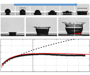
  $\tau < 0.1$). Specifically, the droplet has the shape of a truncated sphere and is surrounded by a thin, radially spreading lamella, in agreement with the numerical simulations of Wildeman et al. (Reference Wildeman, Visser, Sun and Lohse2016). The KD formation occurs at the rim of this lamella, which has a thickness much smaller than the droplet central height. For these conditions, it appears appropriate to model the decay of the liquid layer $h_{tot}(t)$ at the foot of the crown as $h_{tot}(t) = h_{res_D} + h_F(t)$. We found that for impact on wetted walls with $\delta$ in the range $0.06 \leqslant \delta < 0.4$, $h_{res_D}$ can be estimated as $(h_{res_D} / D_0)_{rW} = 0.4 * (h_{res_D} / D_0)_W = 0.4 * 0.7 Re^{-2/5}$. For higher wall-film thicknesses (i.e. $\delta \geqslant 0.4$), the droplet impact phenomenology approaches the deep pool regime, characterised by the formation of a crater within the impact zone. For these conditions, the droplet-liquid layer can no longer freely slide on the wall film owing to the increased wall-film inertia. In this case, the correlation of van Hinsberg et al. (Reference van Hinsberg, Budakli, Göhler, Berberović, Roisman, Gambaryan- Roisman, Tropea and Stephan2010), which includes an explicit dependence of $h_{res_D}$ upon $\delta$, leads to a better agreement with the experimental data. Note, however, that modelling the droplet impact on thick wall films is beyond the focus of the present work.

Figure 7. Early dynamics of the impact phase for an n-hexadecane droplet with  $\delta = 0.08$, $We_D=1343$, $Re_D=2459$ (exp. No. 3, see Appendix B).
The decay of the wall-film height  $h_F(t)$ in the inertial regime is modelled with the analytical solution of Yarin & Weiss (Reference Yarin and Weiss1995), see (2.7) for more details, until a residual film thickness $h_{res_F}$ is attained. The latter can be estimated on the basis of simple scaling arguments (Lagubeau et al. Reference Lagubeau, Fontelos, Josserand, Maurel, Pagneux and Petitjeans2012). Specifically, $h_{res_F}$ should be proportional to the boundary layer height ( $h_{res_F} \sim h_0 / \sqrt {U_0 h_0 / \nu } \sim h_0 / \sqrt {Re_h}$) and also a fraction of the initial film thickness ( $h_{res_F} \sim \delta$). Hence, the simplest estimation gives $h_{res_F} = 1.5 \, \delta \, h_0 / \sqrt {Re_h}$, where the factor 1.5 is slightly smaller than the boundary layer height [ $h_{BL}/h_0 = 2.5 / \sqrt {Re_h}$] in the transformed coordinate for a stagnation point flow (see figure 5a). Finally, in agreement with the remarks of Lagubeau et al. (Reference Lagubeau, Fontelos, Josserand, Maurel, Pagneux and Petitjeans2012), we would like to point out that this modelling choice is not univocally defined. The two possible dependencies for the residual thickness, $Re^{-1/2}$ or $Re^{-2/5}$, are so close to each other that each of them can be adopted without any loss of accuracy by simply modifying the coefficient of proportionality. The only important requirement is the overall estimation of $h_{tot}(t)$. For the present investigations, we found an excellent agreement with the tabulated residual thicknesses as measured by van Hinsberg et al. (Reference van Hinsberg, Budakli, Göhler, Berberović, Roisman, Gambaryan- Roisman, Tropea and Stephan2010) for $\delta > 0.2$.
2.5. Initialisation
To finalise the modelling of the crown propagation, it is necessary to determine the initial parameters [ $\tau _{ini},\bar {R}_{KD,ini}$] that appear in (2.18). In this work, we start from the asymptotic velocity distribution in the impact zone $F(\zeta ) = {\rm d} \zeta / {\rm d}t = a_0 \zeta$, as it is primarily responsible for the formation of the crown. As shown in figure 7, the KD is located directly at the end of the impact length $L_{im}$. We assume the asymptotic solution $F(\zeta )$ to be valid as of $\tau _{ref}$. Its integration over the length of the impact zone provides the location of the crown at the end of the impact phase (Phase 2). Integrating over the interval $L(\tau _{ref}) = D_0$ until $L(\tau _{ini}) = L_{im}$ yields
 \begin{equation} \ln \left (\frac{L_{im}}{D_0} \right ) = \ln (\alpha) = \lambda (\tau_{ini} - \tau_{ref}), \end{equation}
being  $L_{im}/D_0 = \alpha$ per definition of the impact length. Here, it is important to recall the discussion presented in § 2.1 on the estimation of the factor $\alpha$, based on a comparison between analytical/numerical solutions and empirical correlations. It follows then immediately that $\bar {R}_{KD,ini} = L_{im}/2 =\alpha /2$, while $\tau _{ini}$ can be calculated from (2.19), if the reference time $\tau _{ref}$ can be estimated.
Thoroddsen (Reference Thoroddsen2002) investigated the early dynamics of an ejecta sheet for droplet impact onto a liquid layer. He found that ejecta sheets can emerge as early as  $10\ \mathrm {\mu }{\rm s}$, which, in our experiments, corresponds to $\tau$ values in the range of $0.013 < \tau < 0.019$ depending on the fluid viscosity. We assume that the condition $L(\tau _{ref}) = D_0$ is reached shortly after and chose $\tau _{ref} = 0.02$ for all test cases. To assess the influence of $\tau _{ref}$ on the time initialisation, we performed a parameter study by varying $\tau _{ref}$ in the interval $[3 \times 10^{-3}\text {--}0.14]$ for different initial wall-film heights and test fluids. As can be seen in figure 8, $\tau _{ini}$ is rather insensitive to the choice of $\tau _{ref}$, provided $\tau _{ref} < 0.04$. The choice of $\tau _{ref}$ mainly influences the fraction of droplet volume that penetrates into the wall film. The latter is irrelevant for the chosen initialisation approach and never exceeds a few percent of the droplet volume.

Figure 8. Sensitivity analysis on the prediction of  $\tau _{ini}$: (a) variation of $\delta$; (b) influence of viscosity; (c) fraction of droplet volume penetrated into the wall film at $\tau _{ref}$. To highlight the changes in $\tau _{ini}$, a double logarithmic scale is chosen for all plots.
2.6. Comparison between different initialisation procedures
This section presents a direct comparison between the initialisation method proposed by Gao & Li (Reference Gao and Li2015) and the one proposed in this work (2.19). An overview of the different assumptions is presented in table 2. Gao & Li (Reference Gao and Li2015) employed a volumetric approach, based on the conservation of the droplet volume. The latter is transformed into an equivalent cylinder of base  ${\rm \pi} \bar {r}_i^{2}$ and height $\delta$, where the radial position $\bar {r}_i=1/\sqrt {6\delta }$ denotes the origin of the KD. The initial time is estimated as $\tau _i = (\bar {r}_i -0.5)/ \lambda$. Hence, it follows that $\bar {r}_i=\bar {R}_{KD,ini}$ and $\tau _i=\tau _{ini}$. As shown in figure 7, this assumption is not realistic, because the KD formation starts very early in the impact phase, when only a few percentage of the droplet volume has penetrated into the wall film. The overall disadvantage of the volumetric approach is that it leads to a significant overestimation of both initial parameters for small wall-film thicknesses ( $\delta < 0.2$), as shown in figure 9(a,b). This occurs because increasingly more time is required to transform the droplet volume in an equivalent cylinder of height $\delta$ and radius $\bar {r}_i$. The overestimation of the initial parameters [ $\bar {R}_{KD,ini}, \tau _{ini}$] is confirmed by analysing the early stage dynamics of droplet impact on thin films, shown, for example, in figure 7. Even though only a rough estimation of the formation time can be obtained from the figure, it follows $\tau _{ini} \ll 2$, being $\tau _{ini} =0.087 \times 5=0.435$. This experimental value is well reproduced by our initialisation method, while the initialisation of Gao & Li (Reference Gao and Li2015) predicts a formation time of $\tau _{ini} \approx 2.3$. To compensate for this overestimation, Gao & Li (Reference Gao and Li2015) introduced the parameter $C_{0}(\delta )$ (see figure 9c) in their theoretical prediction. The expression for $C_{0}(\delta )$ is obtained by setting $\bar {R}_{KD}(\tau _{ini})=\bar {r}_i$. Hence, it follows from table 1:
 $$\begin{gather} \bar{R}_{KD}=\beta_{GL} \sqrt{\tau_{ini}}+C_{0}(\delta)=\bar{r}_{i}, \end{gather}$$
 $$\begin{gather}C_{0}(\delta)=\bar{r}_{i}-\beta_{GL} \sqrt{\tau_{ini}}=\frac{1}{\sqrt{6\delta}}-\left(\frac{2\lambda^{2}}{3\delta}\right)^{1/4}\sqrt{\frac{1}{\lambda} \left(\frac{1}{\sqrt{6\delta}}-\frac{1}{2}\right)} , \end{gather}$$
 $$\begin{gather}C_0(\delta)=\frac{1}{\sqrt{6\delta}}-\left(\frac{1}{3\delta}-\frac{1}{\sqrt{6\delta}}\right)^{1/2}. \end{gather}$$
Table 2. Direct comparison of initialisation parameters  $\bar {R}_{KD,ini}$ and $\tau _{ini}$.


Figure 9. Dependence of the initialisation parameters upon the non-dimensional film thickness  $\delta$ for different theoretical models: (a) initial crown radius $\bar {R}_{KD,ini}$; (b) initial time $\tau _{ini}$; (c) parameter $C_{0}(\delta )$.
The dependence of  $C_{0}$ on the non-dimensional film thickness $\delta$ is depicted in figure 9(c). For thin films ( $\delta <0.17$), the parameter $C_{0}(\delta )$ assumes negative values, which limits the temporal applicability of the Gao & Li correlation (see correlation No. 2 in table 1). In other words, $\bar {R}_{KD}$ cannot assume negative values. As shown in figure 2(b) and in § 3, the offset $C_{0}(\delta )$ leads to a correct positioning of the theoretical curve for $0.1<\delta <0.3$ for which the model was validated. Outside of this range, the following is observed. For $\delta <0.1$, $\tau _{ini}$ is too large, as shown in figures 11(a) and 12(a). For $\delta \geqslant 0.3$, the slope of the $\bar {R}_{KD}$-curve is underestimated owing to the vertical shift in the $\sqrt {\tau }$-curve (see (2.20)), induced by the artificial offset. This is demonstrated by comparing the slope of all $\bar {R}_{KD}$-curves close to the initialisation point with the experimental data for $\delta =0.3$ (see e.g. figures 11b and 12b).
In our approach,  $\tau _{ini}$ is estimated by (2.19), while $\bar {R}_{KD,ini}$ is directly connected to the length of the impact zone: $\bar {R}_{KD,ini} = \alpha /2$. The latter was estimated by comparing the analytical solution to the available empirical correlations under the assumption that the extent of the impact zone is limited by friction effects for $\delta \leqslant 0.2$ and by wall-film inertia for $\delta > 0.2$, as explained in §§ 2.1 and 2.5. Despite these limitations, in § 3, it is shown that the newly proposed initialisation provides a significant improvement compared with previous estimations and exhibits an excellent agreement with experimental data over the entire range of wall-film thicknesses considered in this work ( $0.03 \leqslant \delta < 0.4$).
3. Results and discussions
The objectives of this section are twofold. First, it is necessary to verify the existence of self-similar solutions in the transformed coordinate system for the unsteady stagnation point flow with decaying strength  $a(t)$. Second, the predictive capabilities of (2.18) in reproducing the temporal evolution of the dimensionless crown radius $\bar {R}_{KD}$ need to be assessed. Concerning the self-similarity, the radial momentum equation in the transformed coordinate system (i.e. (2.13)) has been solved twice for a selected n-hexadecane experiment (Exp. No. 5 in table 3). The two solutions differ only in the modelling of the unsteady term, as discussed in detail in § 2.2. Specifically, in the first approach, the parameter $1/a(t)$ is kept constant by setting $1/a(t) = 1/ a_0 = {\rm const}.$; while in the second approach, the temporal variation of the parameter $a(t)$ is explicitly incorporated by repeating the iterative solution of (2.13) at each time step. The result of this exercise is shown in figure 10. As can be seen, the two solutions overlap perfectly. This confirms the order of magnitude analysis presented in § 2.2. Specifically, it was shown that the overlapping of the different profiles (self-similarity requirement) is directly related to the negligibility of the unsteady term in the transformed coordinate system. In what follows, we make use of the self-similarity by solving (2.13) only once at the nominal impact strength $a_0 = \lambda U_0/D_0$, because the latter can be immediately inferred from the initial impact conditions.

Figure 10. Verification of the self-similarity assumption for the unsteady stagnation point flow with decaying strength  $a(t)$. Test case: experiment No. 5 in table 3.
Concerning the reliability of our viscous correction, the capability of (2.18) in predicting the propagation of the crown radius (KD) is analysed for a variety of fluids, which include hyspin, n-hexadecane and the silicone oils B3, B10 and B50. In total, more than 700 droplet impact experiments were performed and analysed, covering a wide range of normalised wall-film thickness ( $0.03 \leqslant \delta \leqslant 0.5$), droplet Weber number $600 < We_{D} < 1900$ and droplet Reynolds number $160 < Re_{D} < 2600$. Please note that each experiment was repeated five times to evaluate the reproducibility of the crown morphology and spreading rate. A detailed description of the test-rig, experimental procedures, post-processing algorithm and reliability of the experimental data can be found in Geppert et al. (Reference Geppert, Terzis, Lamanna, Marengo and Weigand2017) and Bernard et al. (Reference Bernard, Vaikuntanathan, Weigand and Lamanna2020). The inaccuracy in determining the position of the KD is approximately 1–2 % (Geppert et al. Reference Geppert, Chatzianagnostou, Meister, Gomaa, Lamanna and Weigand2016), while the inaccuracy in the determination of $Re_D$, $We_D$ and $\delta$ is approximately 2.5–3 % (Geppert et al. Reference Geppert, Terzis, Lamanna, Marengo and Weigand2017). Hereafter, only a selected number of experiments are discussed, which span over the entire range of test conditions, and are listed in Appendix B. As pointed out by Geppert et al. (Reference Geppert, Terzis, Lamanna, Marengo and Weigand2017), the crown propagation is only weakly dependent upon the $We_D$ and $Re_D$ numbers. It is, instead, very sensitive to the initial wall-film thickness, which controls, to a large extent, the interplay between viscous and inertial forces.
The predictions of the non-dimensional crown radius  $\bar {R}_{KD}$ for hyspin and the silicone oils B10 and B50 are shown in figure 11, while those for n-hexadecane and B3 are plotted in figure 12. In all cases, a comparison with the experimental data and the model of Gao & Li (Reference Gao and Li2015) is also included. The inclusion of momentum losses reproduces quite accurately the systematic deviation from the $\sqrt {t}$ time dependence observed in the experimental data. Moreover, it leads to a significant improvement in the accuracy of the predictions, particularly in the late spreading phase compared to inviscid models (e.g. Gao & Li Reference Gao and Li2015). Note that the deviation from the inviscid solution occurs at increasingly later times with increasing $\delta$. Consequently, the improvement caused by the inclusion of momentum losses is more pronounced for small, initial wall-film thickness ( $\delta <0.2$). For $\delta > 0.3$, the liquid film acts as a buffer and attenuates the retarding effect of the wall on the outer flow velocity. Indeed, for $\delta = 0.4$ (figure 12c), the experimental data are also well reproduced by the Gao & Li (Reference Gao and Li2015) model for a significant part of the crown evolution. Noteworthy is the counterintuitive role played by viscosity. In figures 11(c) and 11(d), the B50 curve follows more closely the inviscid solution compared with the B10 case for $\delta = 0.3$. This behaviour arises from the compensation between impact and viscous losses. Impact losses are higher for viscous fluids, leading to smaller $\lambda$ and $a_0$ values. This results in a slower decay rate for the wall-film height (i.e. a smaller velocity gradient in the near-wall region) for the B50 droplet and therefore in attenuated viscous losses compared with the B10 test case.

Figure 11. Temporal evolution of the crown  $\bar {R}_{KD}$: comparison between experiments and theoretical models. The vertical line marks the time of maximum crown's height $H_{cr,max}$. Detailed test conditions can be found in table 3 in Appendix B. (a) Hyspin, $\delta <0.1$. (b) Hyspin, $\delta >0.1$. (c) Silicone oil, B10. (d) Silicone oil, B50.

Figure 12. Temporal evolution of the crown  $\bar {R}_{KD}$: comparison between experiments and theoretical models. The vertical line marks the time of maximum crown's height $H_{cr,max}$. Detailed test conditions can be found in table 3 in Appendix B. (a) n-Hexadecane, $\delta <0.1$. (b) n-Hexadecane, $0.1<\delta <0.3$. (c) n-Hexadecane, $\delta >0.3$. (d) Silicone oil, B3.
These considerations are further corroborated by a direct comparison of the KD velocities predicted by the viscous and inviscid model, respectively. The dependence upon the initial film thickness is analysed in figure 13(a). As can be seen, the largest differences are obtained for small values of the dimensionless wall-film height (e.g.  $\delta = 0.05$) owing to the increased relevance of boundary layer effects, while only minor deviations are observed for $\delta = 0.3$. The dependency upon fluid viscosity is illustrated in figure 13(b), which confirms our previous statement about the contrasting effect between impact and viscous losses. Namely, higher impact losses are associated with higher fluid viscosities and lead to reduced viscous losses. Indeed, for a given $\delta$, the B3 silicone oil (red solid curve) experiences basically the same momentum attenuation as the B50 silicone oil (red dashed curve), despite the large differences in kinematic viscosities. Note that, in the early stage of the spreading phase (i.e. $\tau \leqslant 3$), the velocity predictions are basically identical. The time shift observed in the initial phase (see figure 13a) arises from the different initialisation approaches discussed in § 2.6, which differ significantly for droplet impact on thin films (i.e. $\delta < 0.1$). Overall, the comparison shows that our analytical solution is capable of describing the progressive transition from the inertia-controlled to the shear-controlled regime of crown propagation.

Figure 13. Temporal evolution of the KD velocity with ( $\bar {u}^{v}_{KD}$) and without ( $\bar {u}_{KD}$) viscous attenuation for different (a) initial film thicknesses exp. No. 2,6, see Appendix B and (b) fluid viscosities exp. No. 16,22, see Appendix B.
An additional interesting aspect is the direct comparison with correlations developed for droplet impact on dry walls, as shown in figures 11(a) and 12(a) for very thin initial wall-film thicknesses ( $\delta \leqslant 0.04$). Two correlations are considered: a numerically derived one by Philippi et al. (Reference Philippi, Lagrée and Antkowiak2016) and an experimentally derived one by Rioboo et al. (Reference Rioboo, Marengo and Tropea2002). For early times ( $\tau <3$), both the present model (2.18) and the dry wall correlations reproduce the experimental data quite well. For larger times, however, the dry wall correlations start to deviate from the experimental data. This is not surprising because both correlations were validated only in the range $0<\tau <0.1$. The improved predictions of (2.18) arise from the inclusion of viscous losses, which become relevant at later times ( $\tau >3$). The comparison with dry wall correlations demonstrates that (2.18) is also capable to predict the crown radius evolution for both dry and wetted wall impacts.
Regarding the occurrence of crown retraction, the latter is caused by the restoring action of surface tension. As mentioned in § 1, this may also cause deviations from the square-root time dependence. Our experimental results show that crown retraction is not observed systematically. This occurs because, during a splashing event, the crown may collapse or break before a balance between inertia and capillary forces is reached. Typically, this is the case for droplet impact on very thin films, as shown in figure 14. For hyspin, for example, the crown is ripped off at its base already during the early stage of the elevation phase, namely at  $\tau = 7.8$. In figures 11 and 12, the occurrence of crown retraction coincides with a decrease in time of the crown base radius. For these cases, our analytical solution is no longer capable to follow the experimental trend. Noteworthy is the fact that crown retraction develops only after the crown velocity has decayed to almost zero, as illustrated by the horizontal slope in e.g. figure 11(b,c) for $\delta = 0.2$. Our experimental results seem to suggest that crown retraction can occur only when inertia and viscous forces become negligible due to the vanishing crown speed. If that happens, surface tension remains the only dominant force and is capable to reverse the crown motion against wall friction effects.

Figure 14. Crown bottom breakup time sequence with  $\delta = 0.05$ (exp. No. 2 and 10 in Appendix B).
4. Conclusions
In this work, an extension of the potential flow solution that describes the propagation of the crown (Yarin & Weiss Reference Yarin and Weiss1995) is presented. Although not explicitly stated in the original model, the potential flow has the structure of a stagnation point flow of constant strength in the impact phase (Phase 1). During the spreading phase (Phase 3), instead, due to the exponential decay of the peak impulse provided by the impacting droplet (Mitchell et al. Reference Mitchell, Klewicki, Korkolis and Kinsey2019), the potential flow evolves towards an unsteady stagnation point flow with decaying strength  $a(t) = a_0 /(1+a_0 t)$. Our strategy has been first to recover the original solution for the crown propagation $\bar {u}_{KD}$, based on the above mentioned outer flow structure. Second, we extended it by integrating a boundary layer correction to describe the momentum reduction due to viscous losses. For this purpose, we solved analytically the Navier–Stokes equations and found a self-similar solution in the variables $[r \sqrt {a(t)/(\nu t)}, z \sqrt {a(t)/(\nu t)} ]$ for $a_0 \geqslant 100\ {\rm s}^{-1}$. The latter represents a straightforward generalisation of the self-similar, inviscid stagnation point flow solution in the variables $(r / \sqrt {t}, z / \sqrt {t})$ (Philippi et al. Reference Philippi, Lagrée and Antkowiak2016). The consistent application of the outer flow solution in the impact zone leads to an accurate determination of the extent of the impact region and required time $\tau _{ini}$ for the formation of the KD. Our analysis shows that, during the spreading phase, viscous losses are negligible only in the early stage of crown propagation and become increasingly important with reducing film height. This causes a systematic variation from the square-root time dependence, derived from the inviscid approach. Our study also showed that viscous losses affect the temporal evolution of the crown in two ways: directly by causing momentum losses during the spreading of the lamella and indirectly through the impulse transfer from the droplet to the wall film, which is inhibited in highly viscous fluids. This generates a complex interaction between impact and viscous losses: the higher the impact losses, the lower the total viscous losses in the spreading phase and vice versa. This counterbalancing of impact and viscous losses explains why the crown evolution was found to be only weakly dependent upon fluid viscosity.
Funding
The authors wish to thank the Deutsche Forschungsgemeinschaft (DFG) for financial support in the framework of the project GRK 2160/1 ‘Droplet Interaction Technologies’ (DROPIT), under project number 270852890.
Declaration of interests
The authors report no conflict of interest.
Appendix A. Exact derivation of the unsteady term
In this section, we present the exact derivation of the unsteady term in the transformed coordinate system and discuss its influence on the solution of the self-similar function  $g(\xi )$.
Proof. Recalling the definition of the vertical, transformed coordinate  $\xi = [z \sqrt {a(t) / (\nu t)} ]$, the proof is as follows:
 \begin{align} \frac{\partial u}{\partial t} & = \frac{\partial }{\partial t} \left[ \frac{a(t) \, r}{t} g' \left( \xi \right ) \right ] \nonumber\\ & = \frac{a(t) \, r}{t} g''(\xi) \frac{\partial }{\partial t} \left[ \sqrt{\frac{a(t)}{\nu t}} z \right ] + g'(\xi) \frac{\partial }{\partial t} \left[ \frac{a(t) r}{t} \right ] \nonumber\\ & ={-} \frac{a(t) \, r}{t^{2}} \frac{\xi }{2} g''(\xi) - \frac{a(t)^{2} \, r}{t} \frac{\xi }{2} g''(\xi) + g'(\xi) \left[ - \frac{a(t) \, r}{t^{2}} - \frac{a(t)^{2} \, r}{t} \right ] \nonumber\\ & ={-} g''(\xi) \frac{a(t) \, r}{t^{2}} \frac{\xi }{2} [1+a(t) t] - g'(\xi) \frac{a(t) \, r}{t^{2}} [1+a(t) t] \nonumber\\ & ={-} \frac{a(t) \, r}{t^{2}} \left ( \frac{\xi}{2} g'' + g' \right ) \left [1 + \frac{a_0 t}{(1+ a_0 t)} \right ] \end{align}
 \begin{align} & ={-} \frac{a(t) \, r}{t^{2}} \left ( \frac{\xi}{2} g'' + g' \right ) \left [1 + \varepsilon(t) \right ]. \end{align}
Appendix B. Test conditions and fluid properties
In this section, the experimental conditions of the analysed experiments are listed.
Table 3. Listing of experimental parameters for n-hexadecane and hyspin experiments. More details on the experimental set-up can be found in Geppert et al. (Reference Geppert, Terzis, Lamanna, Marengo and Weigand2017).

Table 4. Listing of experimental parameters for silicone oil B3, B10 and B50 experiments. More details on the experimental set-up can be found in Bernard et al. (Reference Bernard, Vaikuntanathan, Weigand and Lamanna2020).


 Open access