


1. Introduction
One of the most fundamental problems in fluid dynamics that has evaded a general solution is describing the unsteady motion of particles immersed in a prescribed background flow. Most analytical attempts work under the severe assumption of unsteady Stokes flows, for which symmetry-breaking inertial effects are neglected (see Michaelides (Reference Michaelides1997) for a brief overview). Following the pioneering contributions of Basset (Reference Basset1888), Boussinesq (Reference Boussinesq1885) and Oseen (Reference Oseen1927) for uniform background flows, resulting in what is now termed the BBO equation, effects of flow non-uniformity were taken into account by Gatignol (Reference Gatignol1983) and Maxey & Riley (Reference Maxey and Riley1983) (MR). Because of its comprehensive, rigorous and systematic character, MR has been widely used to describe hydrodynamic forces on particles over the past 40 years, although it still operates strictly in the limit of vanishing inertial effects.
The Maxey–Riley equation for spherical particles (MR equation) assumes the validity of the unsteady Stokes assumption, which implies that (i) the particle Reynolds number based on a typical difference velocity between particle speed and background flow must be small, and (ii) the background flow gradients must be small compared with viscous momentum diffusion. These assumptions do constrain the applicability of MR in a number of situations. One of the most glaring shortcomings was pointed out by Leal (Reference Leal1992), and concerns the incompatibility of MR with the experimentally observed phenomenon of lateral migration of particles due to lift forces caused by inertial effects. Subsequent work aimed at the development of equations valid at finite particle Reynolds numbers has yielded specialized results, for example for steady flow (Ho & Leal Reference Ho and Leal1974; Martel & Toner Reference Martel and Toner2014; Hood, Lee & Roper Reference Hood, Lee and Roper2015) or for forces occurring in acoustic fields (Baudoin & Thomas Reference Baudoin and Thomas2020; Rufo et al. Reference Rufo, Cai, Friend, Wiklund and Huang2022).
The advent of oscillatory microfluidics (Lutz, Chen & Schwartz Reference Lutz, Chen and Schwartz2003; Marmottant & Hilgenfeldt Reference Marmottant and Hilgenfeldt2003; Thameem, Rallabandi & Hilgenfeldt Reference Thameem, Rallabandi and Hilgenfeldt2017; Mutlu, Edd & Toner Reference Mutlu, Edd and Toner2018; Zhang et al. Reference Zhang, Bachman, Ozcelik and Huang2020, Reference Zhang, Song, Bai, Guo, Feng and Arai2021a,Reference Zhang, Song, Bai, Jia, Song, Guo and Fengb, Reference Zhang, Allegrini, Yanagisawa, Deng, Neuhauss and Ahmed2023) has since introduced the use of much stronger particle inertia effects, enabling fast and high-throughput particle manipulation. Yet again, quantitative modelling and prediction of such effects has been largely lacking, with experimental results often explained qualitatively, and/or by appealing to analogies with theories that are not obviously applicable, such as particle forces in acoustofluidics (Gor'kov Reference Gor'kov1962; Friend & Yeo Reference Friend and Yeo2011; Devendran, Gralinski & Neild Reference Devendran, Gralinski and Neild2014; Chen et al. Reference Chen, Fang, Merritt, Strack, Xu and Lee2016; Nadal & Lauga Reference Nadal and Lauga2016; Collins et al. Reference Collins, O'Rorke, Neild, Han and Ai2019; Wu et al. Reference Wu, Ozcelik, Rufo, Wang, Fang and Jun Huang2019). Given the versatility and richness of microfluidic flows, what is needed is a fundamental understanding of inertial hydrodynamic forces acting on particles immersed in a general unsteady background flow, that is, a true generalization of MR.
In a first step towards such a generalization, Agarwal et al. (Reference Agarwal, Chan, Rallabandi, Gazzola and Hilgenfeldt2021) rigorously described inertial forces on density-matched particles. Whereas MR does not predict any net force on neutrally buoyant particles immersed in unsteady fluid flows, Agarwal et al. (Reference Agarwal, Chan, Rallabandi, Gazzola and Hilgenfeldt2021) showed that such a force can be very significant and is often dominant in oscillatory microfluidics. In the present paper, we augment that formalism to include finite density contrast between particle and fluid (a relevant scenario in microfluidics), thus completing the consistent generalization of MR. In our theory, density-contrast dependent contributions to inertial forces specialize to the well-known Auton correction (Auton, Hunt & Prud'Homme Reference Auton, Hunt and Prud'Homme1988) in the potential flow limit, but continue to play a significant role in the presence of unsteady viscous effects. In a different specific limit our framework establishes a quantitative connection with acoustofluidic formulae for radiation forces on particles, which, as has been remarked above, have up to now been used in an unsystematic way in oscillatory microfluidics.
The organization of this paper is as follows. In § 2 we describe the general theoretical formalism for inertial forces and their evaluation for oscillatory flows. In § 3, we develop an explicit time-averaged equation of motion for spherical particles, and in § 4 we rigorously compare its predictions with direct numerical simulations (DNS) as well as with existing theories in specialized limits. Section 5 discusses the validity and importance of the present approach in practical situations, while § 6 draws conclusions.
2. Theoretical formalism
2.1. Problem set-up
In this paper we develop a unifying theory for the equation of motion of spherical particles of radius  $a_p$ and mass $m_p$ immersed in general unsteady incompressible Newtonian flows of fluid density $\rho _f$ (figure 1), placing particular emphasis on fast oscillatory flows, while consistently accounting for particle inertia. The characteristic speed $U^*$ of the unsteady background flow evaluated at the particle position and kinematic viscosity $\nu$ of the fluid define the particle Reynolds number ${Re}_{p}=a_p U^*/\nu$. The particle reaction to the flow importantly also depends on the Stokes number, which we define as $\lambda =a_p^2\omega /(3\nu )$. The unsteady time scale of the flow is written as $1/\omega$, anticipating the oscillatory case, where we can alternatively use the Stokes boundary layer scale $\delta =(2\nu /\omega )^{1/2}$ to write $\lambda =2a_p^2/3\delta ^2$.

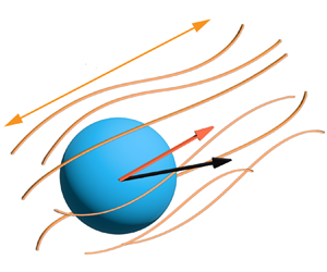
Figure 1. (a) Schematic of a spherical particle of radius  $a_p$ moving with a velocity $\boldsymbol {U}_p$ as a consequence of the hydrodynamic force $\boldsymbol {F}$ exerted by the surrounding fluid. The undisturbed flow field far away from the particle is denoted by $\boldsymbol {U}$. The hydrodynamic force is generally decomposed into a force due to the undisturbed flow $\boldsymbol {F}^{(0)}$ and the disturbance flow $\boldsymbol {F}^{(1)}$ due to the presence of the particle. (b) The unsteadiness of the flow introduces the Stokes number $\lambda$, which, for oscillatory flows, is a function of the ratio of the particle size to the oscillatory boundary layer thickness $\delta$. The background flow is Taylor-expanded around the particle centre up to the quadratic term.
We follow MR in decomposing the flow around the particle into the given background flow  $\boldsymbol {U}$ present without the particle, and the disturbance flow due to the particle's presence. Forces caused by the background flow will carry the superscript ${(0)}$, while those stemming from the disturbance flow will have the superscript ${(1)}$. All forces will be computed for arbitrary $\lambda$ and to first order in $Re_p$, using a regular perturbation expansion. In general flows, such an approach is valid in an inner region, while an outer region (in which inertia reasserts dominance) would have to be treated separately and the complete problem solved by asymptotic matching. However, as shown by Lovalenti & Brady (Reference Lovalenti and Brady1993), an outer region is not present when the oscillatory inertia of the disturbance flow is much greater than its advective inertia. We explain in detail below (see § 5.1) how this condition yields explicit criteria for validity across the range of $\lambda$ values. In oscillatory microfluidics, where we typically have $\lambda \sim 1\unicode{x2013}10$, the resulting criteria are comfortably fulfilled for practically relevant flows, so that it is sufficient to demonstrate the solution by regular expansion. Acoustofluidic devices generally operate at $\lambda \gg 1$, and we will show that particle motion in those cases is also quantitatively covered by our formalism. The case $\lambda \ll 1$ is usually not practically relevant, as the resulting inertial forces on particles become very small.
2.2. Particle motion and fluid flow
Our task is thus to determine explicit expressions of terms in the following equation of motion for the particle velocity  $\boldsymbol {U}_p$:
 \begin{equation} m_p \frac{{\rm d} \boldsymbol{U}_p}{{\rm d}t} = \boldsymbol{F}^{(0)}+\boldsymbol{F}^{(1)} =\boldsymbol{F}^{(0)}_0+{Re}_p\boldsymbol{F}^{(0)}_1+\boldsymbol{F}^{(1)}_0+{Re}_p\boldsymbol{F}^{(1)}_1 + \cdots, \end{equation}
where subscripts denote orders of  ${Re}_{p}$. Note that the decomposition of $\boldsymbol {F}^{(0)}$ is exact (there are no terms of higher order in ${Re}_{p}$; cf. MR), while we truncate the expansion of $\boldsymbol {F}^{(1)}$ at first order. Expressions for $\boldsymbol {F}^{(0)}_0$, $\boldsymbol {F}^{(1)}_0$ and part of $\boldsymbol {F}^{(0)}_1$ are contained in the MR equation, and we determine the remaining terms here.
Hydrodynamic force components are computed from the flow field stresses, as  $\boldsymbol {F}^{(i)}=(F_S/6{\rm \pi} )\oint _S \boldsymbol {n}\boldsymbol{\cdot } \boldsymbol {\sigma }^{(i)} \,{\rm d}S$ with $i=0,1$, where we use the Stokes drag scale $F_S/6{\rm \pi} =\nu \rho _f a_p U^*$, and the integral is over the particle surface with its outward normal $\boldsymbol {n}$. We use lowercase letters for velocities non-dimensionalized by $U^*$ and it is advantageous in intermediate results to evaluate these velocities in a coordinate system moving with the particle centre, writing $\boldsymbol {w}^{(0)}=\boldsymbol {u}-\boldsymbol {u}_p$ for the undisturbed background flow and $\boldsymbol {w}^{(1)}$ for the disturbance flow. The dimensionless fluid stress tensors are thus written $\boldsymbol {\sigma }^{(i)}=-p^{(i)}\boldsymbol {I} + \boldsymbol {\nabla } \boldsymbol {w}^{(i)} + (\boldsymbol {\nabla } \boldsymbol {w}^{(i)})^{\rm T}$.
The Navier–Stokes equations in the particle frame of reference can be decomposed into background and disturbance components exactly (without approximations),
 $$\begin{gather} \nabla^{2} \boldsymbol{w}^{(0)}-\boldsymbol{\nabla} p^{(0)} = 3\lambda \left(\frac{\partial \boldsymbol{w}^{(0)}}{\partial t}+\frac{{\rm d} \boldsymbol{u}_p }{{\rm d}t}\right)+{Re}_{p}\left(\boldsymbol{w}^{(0)} \boldsymbol{\cdot } \boldsymbol{\nabla}\boldsymbol{w}^{(0)}\right)\!, \quad \boldsymbol{\nabla} \boldsymbol{\cdot } \boldsymbol{w}^{(0)} =0, \end{gather}$$
 $$\begin{gather}\boldsymbol{w}^{(0)} = \boldsymbol{u}-\boldsymbol{u}_p, \quad \text{as } r \rightarrow \infty, \end{gather}$$
 $$\begin{gather} \begin{aligned}\nabla^{2} \boldsymbol{w}^{(1)}-\boldsymbol{\nabla} p^{(1)} &= 3\lambda \frac{\partial \boldsymbol{w}^{(1)}}{\partial t}\nonumber\\ &\quad +{Re}_{p}\left[\boldsymbol{w}^{(0)} \boldsymbol{\cdot } \boldsymbol{\nabla} \boldsymbol{w}^{(1)}+\boldsymbol{w}^{(1)}\boldsymbol{\cdot } \boldsymbol{\nabla} \boldsymbol{w}^{(0)} +\boldsymbol{w}^{(1)}\boldsymbol{\cdot } \boldsymbol{\nabla}\boldsymbol{w}^{(1)}\right]\!, \end{aligned}\end{gather}$$
 $$\begin{gather} \boldsymbol{\nabla} \boldsymbol{\cdot } \boldsymbol{w}^{(1)} = 0, \end{gather}$$
 $$\begin{gather}\boldsymbol{w}^{(1)} = \boldsymbol{u}_p-\boldsymbol{U}, \quad \text{on } r=1 \quad \text{and} \quad \boldsymbol{w}^{(1)} = 0, \quad \text{as } r \rightarrow \infty. \end{gather}$$
2.3. Forces from background flow
Both the  $O(1)$ and $O({Re}_{p})$ components of $\boldsymbol {F}^{(0)}$ in (2.1) can be evaluated directly using the divergence theorem and the above Navier–Stokes equations valid for the background flow $\boldsymbol {w}^{(0)}$. In laboratory coordinates (see MR; Rallabandi Reference Rallabandi2021) they read
 \begin{equation} \boldsymbol{F}^{(0)}_0= \frac{F_S}{6{\rm \pi}} \int_{V} \left( 3\lambda \partial_t \boldsymbol{u}\right) \,{\rm d}V,\quad \boldsymbol{F}^{(0)}_1=\frac{F_S}{6{\rm \pi}} \int_{V} \left(\boldsymbol{u}\boldsymbol{\cdot } \boldsymbol{\nabla} \boldsymbol{u}\right) \,{\rm d}V. \end{equation}
To make further progress, we need to evaluate forces due to successive orders of  $\boldsymbol {w}^{(1)}$, which are ultimately also derived from the given background field $\boldsymbol {u}$. To render our solution strategy analytically tractable, we expand $\boldsymbol {u}$ around the leading-order particle position $\boldsymbol {r}_{p_0}$ into spatial moments of alternating symmetry,
 \begin{equation} \boldsymbol{u}=\boldsymbol{u}|_{\boldsymbol{r}_{p_0}} + \boldsymbol{r}\boldsymbol{\cdot } \boldsymbol{E} + \boldsymbol{r}\boldsymbol{r}:\boldsymbol{G}+\cdots,\end{equation}
where  $\boldsymbol {E}=(a_p/L_\varGamma )\boldsymbol {\nabla } \boldsymbol {u}|_{\boldsymbol {r}_{p_0}}$ and $\boldsymbol {G}=\tfrac {1}{2}(a_p^2/L_\kappa ^2)\boldsymbol {\nabla }\boldsymbol {\nabla } \boldsymbol {u}|_{\boldsymbol {r}_{p_0}}$ are time-dependent, with gradient $L_\varGamma$ and curvature $L_\kappa$ length scales. Such an expansion is valid for $a_p/L_\varGamma \ll 1$ and $a_p/L_\kappa \ll 1$, conditions readily satisfied in microfluidic scenarios. Based on this, (2.3a,b) was recently evaluated analytically by Agarwal et al. (Reference Agarwal, Chan, Rallabandi, Gazzola and Hilgenfeldt2021) and Rallabandi (Reference Rallabandi2021), showing that an $O({Re}_p)$ contribution from $\boldsymbol {F}^{(0)}_1$ had been missed in MR, while being, in fact, of the same order as other terms in the original MR equation.
2.4. Disturbance flow: zeroth order
The Navier–Stokes equations for the disturbance flow at  $O({Re}_p^0)$ read
 $$\begin{gather} \nabla^{2} \boldsymbol{w}_0^{(1)}-\boldsymbol{\nabla} p_0^{(1)} =3\lambda \frac{\partial \boldsymbol{w}_0^{(1)}}{\partial t}, \quad \boldsymbol{\nabla} \boldsymbol{\cdot } \boldsymbol{w}_0^{(1)} =0, \end{gather}$$
 $$\begin{gather}\boldsymbol{w}_0^{(1)} = \boldsymbol{u}_{p_0}-\boldsymbol{u}, \quad \text{on } r=1 \quad \text{and} \quad \boldsymbol{w}_0^{(1)} = 0 ,\quad \text{as } r \rightarrow \infty. \end{gather}$$
Unlike MR, where the solution to this unsteady Stokes equation (2.5) was not explicitly needed to compute the force resulting from it, our present approach does require expressions for  $\boldsymbol {w}^{(1)}_0$ to compute the full $O({Re}_p)$ force. This is accomplished by substituting the expansion (2.4) into (2.5). Each spatial moment gives rise to a linear equation with known solutions, the sum of which yields the general expression (see Landau & Lifshitz Reference Landau and Lifshitz1959; Pozrikidis et al. Reference Pozrikidis1992)
 \begin{equation} \boldsymbol{w}^{(1)}_0 = \boldsymbol{\mathcal{M}}_D \boldsymbol{\cdot } \boldsymbol{u}_s - \boldsymbol{\mathcal{M}}_Q \boldsymbol{\cdot }\left(\boldsymbol{r}\boldsymbol{\cdot } \boldsymbol{E}\right) -\boldsymbol{\mathcal{M}}_O \boldsymbol{\cdot }\left(\boldsymbol{r}\boldsymbol{r}:\boldsymbol{G}\right) + \cdots, \end{equation}
where  $\boldsymbol {u}_s = \boldsymbol {u}_{p_0}-\boldsymbol {u}\vert _{\boldsymbol {r}_{p_0}}$ is the slip velocity and $\boldsymbol {\mathcal {M}}_{D,Q,O}(r,\lambda )$ are mobility tensors with known spatial dependence. For oscillatory flows, their dependence on the Stokes number $\lambda$ is known analytically. Explicit expressions for these tensors are given in Appendix A.
2.5. Disturbance flow: first order using a reciprocal theorem
Fast oscillatory particle motion can give rise to large disturbance flow gradients, so that terms involving  $\boldsymbol {\nabla }\boldsymbol {w}^{(1)}$ on the right-hand side of (2.2d) are not necessarily negligible compared with the viscous diffusion term on the left-hand side, and $O({Re}_p)$ force terms in $\boldsymbol {F}^{(1)}$ become important.
With  $\boldsymbol {w}^{(1)}_0$ explicitly known, the equations at $O({Re}_p)$ read
 $$\begin{gather} \nabla^{2} \boldsymbol{w}^{(1)}_1-\boldsymbol{\nabla} p^{(1)}_1 =\boldsymbol{\nabla} \boldsymbol{\cdot } \boldsymbol{\sigma}^{(1)}_1=3\lambda \frac{\partial \boldsymbol{w}^{(1)}_1}{\partial t}+\boldsymbol{f}_0, \quad \boldsymbol{\nabla} \boldsymbol{\cdot } \boldsymbol{w}^{(1)}_1 =0, \end{gather}$$
 $$\begin{gather}\boldsymbol{w}^{(1)}_1 =-\boldsymbol{u}_{p_1}, \quad \text{on } r=1 \quad \text{and} \quad \boldsymbol{w}^{(1)}_1 = 0, \quad \text{as }\quad r \rightarrow \infty , \end{gather}$$
with  $\boldsymbol {f}_0=\boldsymbol {w}^{(0)}_0\boldsymbol{\cdot } \boldsymbol {\nabla } \boldsymbol {w}^{(1)}_0+\boldsymbol {w}^{(1)}_0\boldsymbol{\cdot } \boldsymbol {\nabla } \boldsymbol {w}^{(0)}_0 +\boldsymbol {w}^{(1)}_0\boldsymbol{\cdot } \boldsymbol {\nabla }\boldsymbol {w}^{(1)}_0$ as the leading-order nonlinear forcing.
In order to compute the force  $\boldsymbol {F}^{(1)}_1$, we do not solve for the flow field $\boldsymbol {w}^{(1)}_1$ in (2.7) but instead employ a reciprocal relation in the Laplace domain. The reciprocal theorem infers the force from the known stress of a test flow $\boldsymbol {u}'$, which is here chosen to be a dipolar unsteady Stokes flow around the particle with arbitrary directionality $\boldsymbol {e}$; see Appendix B for a detailed derivation. We obtain for the magnitude of the force along ${\boldsymbol {e}}$,
 \begin{equation} \boldsymbol{e}\boldsymbol{\cdot } \boldsymbol{F}^{(1)}_1 = \frac{F_S}{6{\rm \pi}}\mathcal{L}^{-1}\left\{\int_{S_p}\frac{\hat{\boldsymbol{u}}_{p_1}}{\hat{u}'}\boldsymbol{\cdot } \left( \hat{\boldsymbol{\sigma}}'\boldsymbol{\cdot } \boldsymbol{n}\right)\,{\rm d}S - {Re}_p\int_V \frac{\hat{\boldsymbol{u}}' \boldsymbol{\cdot } \hat{\boldsymbol{f}}_0}{\hat{u}'}\,{\rm d}V \right\}\!,\end{equation}
where the hat denotes the Laplace transform and  $\mathcal {L}^{-1}$ is the inverse Laplace transform. When applied at $O(1)$, this reciprocal-theorem strategy similarly yields
 \begin{equation} \boldsymbol{e}\boldsymbol{\cdot } \boldsymbol{F}^{(1)}_0 =F^{(1)}_0= \frac{F_S}{6{\rm \pi}}\mathcal{L}^{-1}\left\{\int_{S_p}\frac{\hat{\boldsymbol{w}}_0^{(0)}}{\hat{u}'}\boldsymbol{\cdot } \left( \hat{\boldsymbol{\sigma}}'\boldsymbol{\cdot } \boldsymbol{n}\right)\,{\rm d}S\right\} , \end{equation}
which is precisely the force expression obtained by MR. Since the variable in the overall equation of motion (2.1) is the unexpanded particle velocity  $\boldsymbol {u}_{p}$, we make the substitution $\boldsymbol {w}^{(0)}_0=\boldsymbol {w}^{(0)} - {Re}_p \boldsymbol {u}_{p_1}+O({Re}_p^2)$. Adding (2.9) and (2.8), the $O({Re}_p)$ term in (2.9) exactly cancels the first term in (2.8) and produces a correction term that is $O({Re}_p^2)$. The net force on the particle due to its disturbance flow then reads
 $$\begin{gather} \boldsymbol{e}\boldsymbol{\cdot } \boldsymbol{F}^{(1)} = \boldsymbol{e}\boldsymbol{\cdot } \left(\boldsymbol{F}^{(1)}_0+{Re}_p\boldsymbol{F}^{(1)}_1\right) +O({Re}_p^2), \end{gather}$$
 $$\begin{gather}\boldsymbol{e}\boldsymbol{\cdot } \boldsymbol{F}^{(1)}_0= \frac{F_S}{6{\rm \pi}}\mathcal{L}^{-1}\left\{\int_{S_p}\frac{\hat{\boldsymbol{w}}^{(0)}}{\hat{u}'}\boldsymbol{\cdot } \left( \hat{\boldsymbol{\sigma}}'\boldsymbol{\cdot } \boldsymbol{n}\right)\,{\rm d}S\right\}\!, \end{gather}$$
 $$\begin{gather}\boldsymbol{e}\boldsymbol{\cdot } \boldsymbol{F}^{(1)}_1= \frac{F_S}{6{\rm \pi}}\mathcal{L}^{-1}\left\{- {Re}_p\int_V \frac{\hat{\boldsymbol{u}}' \boldsymbol{\cdot } \hat{\boldsymbol{f}}_0}{\hat{u}'}\,{\rm d}V \right\}\!, \end{gather}$$
where we have also replaced  $\boldsymbol {w}^{(0)}_0$ by $\boldsymbol {w}^{(0)}$ in $\boldsymbol {f}_0$, resulting in an error that is again $O({Re}_p^2)$. Only certain products in $\boldsymbol {f}_0$ are non-vanishing when the angular integration is performed due to alternating symmetry of terms in the background flow field multipole expansion (2.4). These non-zero terms are conveniently labelled by the multipole orders involved in the product
 \begin{equation} {Re}_p\frac{F_S}{6{\rm \pi}}\mathcal{L}^{-1}\left\{-\int_V \frac{\hat{\boldsymbol{u}}' \boldsymbol{\cdot } \hat{\boldsymbol{f}}_0}{\hat{u}'}\,{\rm d}V\right\}= F_{\sigma \varGamma}^{(1)}+ F_{\varGamma\kappa}^{(1)} + \cdots.\end{equation}
Here,  $F_{\sigma \varGamma }^{(1)}$, $F_{\varGamma \kappa }^{(1)}$ are the inertial force contributions obtained by successive contractions of adjacent tensors involving $\boldsymbol {u}_s$ (index $\sigma$), $\boldsymbol {E}$ (index $\varGamma$), $\boldsymbol {G}$ (index $\kappa$) and so on. The volume integral is tedious but straightforward to compute since all the integrations resulting from the leading-order velocity fields (2.4) and (2.6) are convergent. The evaluation of the Laplace transforms can be performed analytically if the flow has harmonic time dependence. This is not a severe restriction as arbitrary time dependences can be decomposed into harmonic contributions. Rectified forces resulting from averaging time-periodic processes can then be computed separately by frequency. Such cases of oscillatory flow are the most relevant in practical applications and are focused on in § 3 below. To simplify notation, we therefore assume a single oscillatory frequency $\omega$ in the following, without loss of generality.
When the particle is neutrally buoyant, the first term  $F_{\sigma \varGamma }^{(1)}$ vanishes so that the leading term is $F_{\varGamma \kappa }^{(1)}$, which was derived in Agarwal et al. (Reference Agarwal, Chan, Rallabandi, Gazzola and Hilgenfeldt2021) as an unexpected inertial force for density-matched particles. This term (involving the product $\boldsymbol {E} : \boldsymbol {G}$) has no analogue in the previous literature and for completeness, we reproduce it as follows for harmonic oscillatory flows $\boldsymbol {U}$:
 \begin{equation} F_{\varGamma \kappa}^{(1)}=m_f a_p^2 \left[\boldsymbol{\nabla}\boldsymbol{U}:\boldsymbol{\nabla}\left(\boldsymbol{\nabla} \boldsymbol{U}\right)\right]\boldsymbol{\cdot } \boldsymbol{e} \mathcal{F}^{(1)}_1. \end{equation}
The  $\lambda$-dependent dimensionless function $\mathcal {F}^{(1)}_1$ results from the volume integration, which also yields $m_f$, the mass of fluid displaced by the particle, via $(4{\rm \pi} a_p^3/3){Re}_p F_S/(6{\rm \pi} ) = m_f a_p^2 (U^*)^2$. In the next section, we follow a similar strategy for non-neutrally buoyant particles.
2.6. Disturbance flow: evaluation of  $F_{\sigma \varGamma }^{(1)}$

Non-neutrally buoyant particles have a slip velocity and thus a non-zero  $F_{\sigma \varGamma }^{(1)}$, involving the product $\boldsymbol {u_s} \boldsymbol{\cdot } \boldsymbol {E}$. Appropriate to fast harmonic oscillatory flows, we approximate the background flow as a potential flow with a given single frequency. The slip velocity as a linear response can then be generally decomposed into an in-phase and an out-of-phase component with respect to the background flow, i.e. $\boldsymbol {u}_s(\boldsymbol {r}_p,t)=\boldsymbol {u}_{s}^{I}(\boldsymbol {r}_p,t)+\boldsymbol {u}_{s}^{O}(\boldsymbol {r}_p,t)$. The corresponding force is written as
 \begin{equation} \frac{F_{\sigma \varGamma}^{(1)}}{{Re}_p F_S/(6{\rm \pi})}=\frac{4{\rm \pi}}{3}(\boldsymbol{u}_{s}^{I}\boldsymbol{\cdot }\boldsymbol{E}) \boldsymbol{\cdot } \boldsymbol{e}\, \mathcal{{G}}_1(\lambda) + \frac{4{\rm \pi}}{3}(\boldsymbol{u}_{s}^{O}\boldsymbol{\cdot }\boldsymbol{E}) \boldsymbol{\cdot } \boldsymbol{e} \mathcal{{G}}_2(\lambda) ,\end{equation}
where the  $\mathcal {{G}}_1$ and $\mathcal {{G}}_2$ terms are explicit outcomes of the volume integration in (2.11) and capture the $\lambda$-dependence of the in- and out-of-phase contributions, respectively. For fast oscillatory background flows, we can replace the in-phase component with $\boldsymbol {u}_{s}\boldsymbol{\cdot }\boldsymbol {E}$ and the out-of-phase component with $\partial _t \boldsymbol {u}_{s}\boldsymbol{\cdot }\boldsymbol {E}$ (see Appendix C for details), resulting in
 \begin{align} F_{\sigma \varGamma}^{(1)} &= \frac{4{\rm \pi}}{3}\rho_f a_p^2 U^{*^2} \left( \boldsymbol{u}_s\boldsymbol{\cdot }\boldsymbol{E} \boldsymbol{\cdot } \boldsymbol{e} \mathcal{G}_1(\lambda) + \partial_t{\boldsymbol{u}_s}\boldsymbol{\cdot }\boldsymbol{E} \boldsymbol{\cdot } \boldsymbol{e} \mathcal{G}_2(\lambda) \right)\nonumber\\ &= m_f \left[ (\boldsymbol{U}_p -\boldsymbol{U})\boldsymbol{\cdot } \boldsymbol{\nabla} \boldsymbol{U}\right]\boldsymbol{\cdot } \boldsymbol{e} \mathcal{G}_1(\lambda) + m_f \left[ \partial_t(\boldsymbol{U}_p -\boldsymbol{U}) \boldsymbol{\cdot } \boldsymbol{\nabla} \boldsymbol{U}\right] \boldsymbol{\cdot } \boldsymbol{e} \frac{\mathcal{G}_2(\lambda)}{\omega}. \end{align}
 While the exact, lengthy expressions for the universal functions  $\mathcal {G}_{1,2}$ are given in Appendix C, an excellent uniformly valid solution can be constructed by simply adding the leading orders of the small and large $\lambda$ expansions of $\mathcal {G}_1$ (analogous to the function $\mathcal {F}$ in Agarwal et al. (Reference Agarwal, Chan, Rallabandi, Gazzola and Hilgenfeldt2021)). Taylor expansion in both the viscously dominated limit ( $\lambda \to 0$) and the inviscid limit ( $\lambda \to \infty$) obtains
 \begin{equation} \mathcal{G}_1^{v} =-\frac{63}{80}\sqrt{\frac{3}{2\lambda}}+O(1),\quad \mathcal{G}_1^{i}=-\frac{1}{2} + O(1/\sqrt{\lambda}), \end{equation}
from which the following uniformly valid result is constructed:
 \begin{equation} \mathcal{G}_1^{uv}(\lambda) \approx-\left(\frac{1}{2} +\frac{63}{80}\sqrt{\frac{3}{2\lambda}}\right)\!. \end{equation}
Figure 2(a,b) illustrates that this simple two-term expression agrees very well with the full result (C3) over the entire range of the parameter  $\lambda$, with a maximum error of ${\sim }6\,\%$.

Figure 2. (a) Plot of the in-phase force function  $\mathcal {G}_1$. The uniformly valid expression (purple dashed) closely tracks the full solution (red). Also displayed are the viscous (green) and inviscid (blue) limit asymptotes. (b) The magnitude of the percentage error between the uniformly valid and full solutions is small throughout the entire range of $\lambda$, with a maximum error of ${\sim }6\,\%$. (c) Plot of the out-of-phase force function $\mathcal {G}_2$ (red) together with its viscous (green) and inviscid (blue) limit expressions.
A Taylor expansion of the out-of-phase term  $\mathcal {G}_2$, in the viscous and inviscid limits, respectively, results in
 \begin{equation} \mathcal{G}_2^v = \frac{3}{16}\sqrt{\frac{3}{2\lambda}} +O(1),\quad \mathcal{G}_2^i =-\frac{57}{40}\sqrt{\frac{3}{2\lambda}} + O(1/\lambda). \end{equation}
Both of the above expansions have a  $O(1/\sqrt {\lambda })$ leading-order term and a simple, two-term approximation fails. In the following, we use the full expression (C4), noting that the contribution from this term is small in most practical situations, i.e. when $\lambda \gtrsim 1$.
3. Equation of motion for a particle immersed in an oscillatory flow
We now collect all the force contributions from (2.3a,b), (2.10c), (2.12), (2.14), and combine them with the results of MR and Agarwal et al. (Reference Agarwal, Chan, Rallabandi, Gazzola and Hilgenfeldt2021). We use dimensional variables for easier physical interpretation. The following is the equation of motion for the velocity  $\boldsymbol {U}_p$ of a rigid spherical particle immersed in an oscillatory background flow field $\boldsymbol {U}$, taking into account all force terms up to $O({Re}_p)$:
 $$\begin{gather} m_p \frac{{\rm d}\boldsymbol{U}_p}{{\rm d}t} = \boldsymbol{F}^{(0)}_0+\boldsymbol{F}^{(1)}_0+ {Re}_p\left(\boldsymbol{F}^{(0)}_1+\boldsymbol{F}^{(1)}_1\right)+O({Re}_p^2), \end{gather}$$
 $$\begin{gather}\boldsymbol{F}^{(0)}_0= m_f \frac{\partial \boldsymbol{U}}{\partial t}, \quad {Re}_p\boldsymbol{F}^{(0)}_1= m_f \left(\boldsymbol{U}\boldsymbol{\cdot }\boldsymbol{\nabla} \boldsymbol{U}\right) + m_f a_p^2 \boldsymbol{\nabla}\boldsymbol{U}:\boldsymbol{\nabla}\left(\boldsymbol{\nabla} \boldsymbol{U}\right)\mathcal{F}^{(0)}_1,\end{gather}$$
 $$\begin{gather}\begin{aligned}\boldsymbol{F}^{(1)}_0&=- \frac{1}{2}m_f \frac{{\rm d}}{{\rm d}t}\left[\boldsymbol{U}_p-\boldsymbol{U}\right] - 6{\rm \pi} \rho_f \nu a_p \left[\boldsymbol{U}_p(t) - \boldsymbol{U}(\boldsymbol{r}_p(t),t) \right] \nonumber\\ &\quad - 6{\rm \pi}^{1/2} \nu^{1/2} a_p^2 \rho_f \int_{-\infty}^t \frac{{\rm d}/{\rm d}\tau \left[\boldsymbol{U}_p(t) - \boldsymbol{U}(\boldsymbol{r}_p(t),t)\right]}{\sqrt{t-\tau}}\,{\rm d}\tau,\end{aligned} \end{gather}$$
 $$\begin{gather} \begin{aligned}{Re}_p\boldsymbol{F}^{(1)}_1 &= m_f \left[ (\boldsymbol{U}_p -\boldsymbol{U})\boldsymbol{\cdot } \boldsymbol{\nabla} \boldsymbol{U}\right] \mathcal{G}_1(\lambda) + m_f \left[ \partial_t(\boldsymbol{U}_p -\boldsymbol{U}) \boldsymbol{\cdot } \boldsymbol{\nabla} \boldsymbol{U}\right] \frac{\mathcal{G}_2(\lambda)}{\omega} \nonumber\\ &\quad + m_f a_p^2 \boldsymbol{\nabla}\boldsymbol{U}:\boldsymbol{\nabla}\left(\boldsymbol{\nabla} \boldsymbol{U}\right)\mathcal{F}^{(1)}_1. \end{aligned}\end{gather}$$
Here, we have dropped the contraction with  $\boldsymbol {e}$ in (2.12) and (2.14) to derive $\boldsymbol {F}_0^{(1)}$, since the direction $\boldsymbol {e}$ is arbitrary (cf. the equivalent argument in MR). Equation (3.1b) includes the background flow force term missing from MR mentioned in § 2.3, proportional to $\mathcal {F}^{(0)}_1=1/5$. As we are modelling the oscillatory background flow as potential (cf. § 2.6), Faxén terms proportional to $\nabla ^2{\boldsymbol {U}}$ are absent. For the same reason of irrotational background flow, particle rotation is neglected. Note that the scales of all the inviscid and inertial force terms use $m_f$, while the viscous force terms contain $\nu$ explicitly. In the following, we point out that (3.1), while containing new physics, encompasses a number of earlier results as special cases, clarifying connections between them.
3.1. Generalized Auton correction
We first comment on the limiting case of the well-known correction to MR due to Auton (Auton et al. Reference Auton, Hunt and Prud'Homme1988). The equation of motion derived by MR deviated from previous versions in the form of the convective term in (3.1b), using  $m_f (\boldsymbol {U}\boldsymbol{\cdot }\boldsymbol {\nabla } \boldsymbol {U})$ instead of $m_f (\boldsymbol {U}_p\boldsymbol{\cdot }\boldsymbol {\nabla } \boldsymbol {U})$ – the values of these two derivatives can differ substantially when the Reynolds number is not small. Similarly, Auton et al. (Reference Auton, Hunt and Prud'Homme1988) showed that in the limit of potential flows, the added mass term should read $\tfrac {1}{2}m_f ({{\rm d}\boldsymbol {U}_p}/{{\rm d}t}-{{\rm D}\boldsymbol {U}}/{{\rm D}t})$ instead of $\tfrac {1}{2}m_f ({{\rm d}\boldsymbol {U}_p}/{{\rm d}t}-{{\rm d}\boldsymbol {U}}/{{\rm d}t})$. Again, these two expressions are identical in the zero Reynolds number limit employed by MR, but in flows with substantial inertial effects, they can differ significantly.
Our formalism naturally addresses these concerns through the rigorous treatment of the disturbance flow around the particle. The first term on the right-hand side of (3.1d), involving  $\mathcal {G}_1$, modifies the added mass term in (3.1c) and reproduces the Auton correction (Auton et al. Reference Auton, Hunt and Prud'Homme1988) in the inviscid, potential flow limit ( $\lambda \to \infty$, ${Re}_p\ll 1$), modifying ${{\rm d} \boldsymbol {U}}/{{\rm d}t}$ to ${{\rm D} \boldsymbol {U}}/{{\rm D}t}$, or explicitly,
 $$\begin{gather} -\frac{1}{2}m_f \frac{{\rm d}}{{\rm d}t}\left[\boldsymbol{U}_p-\boldsymbol{U}\right] + m_f \left[ (\boldsymbol{U}_p -\boldsymbol{U})\boldsymbol{\cdot } \boldsymbol{\nabla} \boldsymbol{U}\right] \mathcal{G}_1(\lambda)\nonumber\\ \approx-\frac{1}{2}m_f \left[\frac{{\rm d}}{{\rm d}t}\boldsymbol{U}_p-\frac{{\rm D}}{{\rm D}t}\boldsymbol{U}\right] - \frac{63}{80}\sqrt{\frac{3}{2\lambda}} m_f \left[ (\boldsymbol{U}_p -\boldsymbol{U})\boldsymbol{\cdot } \boldsymbol{\nabla} \boldsymbol{U}\right]\!, \end{gather}$$
where we use the simple two-term approximation (2.16) for  $\mathcal {G}_1$. Thus, instead of heuristically modifying the added mass term, our approach rigorously derives its dependence on $\lambda$. Note that in most practically relevant oscillatory microfluidic flows, the value of $\lambda$ is $O(1\unicode{x2013}10)$, so that the contribution from the second term of (3.2) – capturing the effect of viscous streaming around the particle – results in the inertial force being quite large due to the $1/\sqrt {\lambda }$ scaling.
We note that the second term in (3.1d), involving  $\mathcal {G}_2$, arises due to the out-of-phase component of the slip velocity and thus characterizes diffusion of vorticity from the particle. This term is analogous to the Basset–Boussinesq history force and contributes most prominently when $\lambda \sim O(1)$, while it is subdominant for both small and large $\lambda$.
3.2. Time scale separation and connection to acoustofluidics
Equation (3.1) describes unsteady particle dynamics as an integral equation containing a history integral, which can be explicitly evaluated in special cases, particularly for particles executing purely oscillatory motion. In more general settings, where there is a superposition of slower rectified or transport fluid flows – with a clear separation of scales from the fast oscillatory motion – we can still find an explicit, analytical evaluation of the memory integral by employing the method of multiple scales. This approach results in a simple overdamped equation of motion for the particle that captures the slow dynamics accurately, as outlined in the following (see Appendix D for details).
For flows induced by a localized oscillating source with curvature scale  $a_b$, amplitude $\epsilon a_b$ and angular frequency $\omega$, we non-dimensionalize our equation with $a_b$, $\epsilon a_b \omega$ and $1/\omega$ as characteristic length, velocity and time scales, respectively. Equation (3.1) then reads
 \begin{align} \lambda \left( \hat{\kappa} + 1\right)\frac{{\rm d}^2 \boldsymbol{r}_p}{{\rm d} t^2} &= \epsilon\lambda \frac{\partial \boldsymbol{u}}{\partial t} + \frac{2\lambda}{3} \epsilon^2 \boldsymbol{u}\boldsymbol{\cdot } \boldsymbol{\nabla} \boldsymbol{u} - \frac{\lambda}{3}\epsilon^2 \lambda \boldsymbol{U}_p \boldsymbol{\cdot } \boldsymbol{\nabla} \boldsymbol{u} -\left(\frac{{\rm d} \boldsymbol{r}_p}{{\rm d} t}-\epsilon\boldsymbol{u}\right)\nonumber\\ &\quad + \sqrt{\frac{3\lambda}{\rm \pi}}\int_{-\infty}^t \frac{{\rm d}/{\rm d}\tau \left[{\rm d}\boldsymbol{r}_p(\tau)/{\rm d}\tau - \epsilon\boldsymbol{u}(\boldsymbol{r}_p(\tau),\tau)\right]}{\sqrt{t-\tau}}\,{\rm d}\tau\nonumber\\ &\quad + \frac{2\lambda}{3}\epsilon \mathcal{G}_1 \left(\frac{d \boldsymbol{r}_p}{d t}-\epsilon\boldsymbol{u}\right)\boldsymbol{\cdot } \boldsymbol{\nabla} \boldsymbol{u} + \frac{2\lambda}{3}\epsilon\, \mathcal{G}_2 \partial_t \left(\frac{{\rm d} \boldsymbol{r}_p}{{\rm d} t}-\epsilon\boldsymbol{u}\right)\boldsymbol{\cdot } \boldsymbol{\nabla} \boldsymbol{u} \nonumber\\ &\quad + \frac{2\lambda}{3}\epsilon^2 \alpha^2 \mathcal{F} \boldsymbol{\nabla}\boldsymbol{u}:\boldsymbol{\nabla} \boldsymbol{\nabla} \boldsymbol{u}, \end{align}
where  $\hat {\kappa }=2/3({\rho _p}/{\rho _f}-1)$ is a dimensionless measure of density difference, $\alpha =a_p/a_b$ is the relative particle size and ${{\rm d} \boldsymbol {r}_p}/{{\rm d}t} =\epsilon \boldsymbol {u}_p$. As in Agarwal et al. (Reference Agarwal, Chan, Rallabandi, Gazzola and Hilgenfeldt2021), we write $\mathcal {F}=\mathcal {F}^{(0)}_1+\mathcal {F}^{(1)}_1$.
We employ standard techniques of time scale separation (see Appendix D) to obtain the leading-order overdamped equation of particle motion. Briefly, the fast oscillatory dynamics in (3.3) are time-averaged over the oscillation period and the resulting equation describes the dynamics of the leading-order mean particle position  $\boldsymbol {r}_{p_0}$ on the slow time scale $T=\epsilon ^2 t$,
 \begin{equation} \frac{{\rm d} \boldsymbol{r}_{p_0}}{{\rm d} T}=\frac{\hat{\kappa}\lambda}{(\hat{\kappa}+1)} \mathcal{G}(\lambda) \left\langle \boldsymbol{u} \boldsymbol{\cdot } \boldsymbol{\nabla} \boldsymbol{u}\right\rangle + \frac{2\lambda}{3}\alpha^2 \mathcal{F}(\lambda) \left\langle \boldsymbol{\nabla} \boldsymbol{u}:\boldsymbol{\nabla} \boldsymbol{\nabla} \boldsymbol{u} \right\rangle ,\end{equation}
with  $\mathcal {F}(\lambda )\approx \tfrac {1}{3} + \tfrac {9}{16}\sqrt {{3}/{2\lambda }}$ derived in Agarwal et al. (Reference Agarwal, Chan, Rallabandi, Gazzola and Hilgenfeldt2021) and
 \begin{equation} \mathcal{G}(\lambda)=\frac{(\hat{\kappa}+1)(2(1-\mathcal{G}_1)(d+\hat{\kappa})\lambda^2 +c\left(2\lambda\mathcal{G}_2-3\right))}{3(c^2+(d+\hat{\kappa})^2\lambda^2)},\end{equation}
where  $c = 1+\sqrt {3\lambda /2}$ and $d=1+\sqrt {3/(2\lambda )}$ are expressions resulting from the integration of the history force term (cf. Appendix D for details).
The first term on the right-hand side of (3.4) can be rewritten as  $F_{R}\mathcal {G}(\lambda )$, where $F_{R} = ({\hat {\kappa }\lambda }/{(\hat {\kappa }+1)}) \langle \boldsymbol {u} \boldsymbol{\cdot } \boldsymbol {\nabla } \boldsymbol {u}\rangle$ is a time-averaged force formally identical to the acoustic radiation force induced by an incident sound field with velocity field $\boldsymbol {u}$ (Bruus Reference Bruus2012). In the acoustofluidic context, this velocity field may be caused by an oscillating object (bubble) excited by a primary acoustic wave. The resulting force from the bubble on a distant particle is then often denoted as the secondary radiation force (Doinikov & Zavtrak Reference Doinikov and Zavtrak1996). As the acoustic formalism is based on the assumption of inviscid flow, $\mathcal {G}(\lambda )$ generalizes the far-field inviscid $F_{R}$ to include viscous effects that, as shown below, can change the resulting particle motion quantitatively and qualitatively. Note that $\mathcal {G}(\lambda \to \infty )=1$, recovering the inviscid case, while the viscous limit depends on the density contrast, $\mathcal {G}(\lambda \to 0)=-(1+\hat {\kappa })$.
In the next section, we specialize (3.4) to the simplest case of a background flow induced by a volumetrically oscillating object – a situation commonly encountered in many practical microfluidic set-ups involving acoustically excited microbubbles – and compare our results with DNS.
4. Validation with DNS
We have shown that the present analytical formalism generalizes previous attempts at predicting the behaviour of particles in oscillatory flows. It is crucial to confirm the quantitative accuracy of our model. To this end, we compare our analytical predictions with independent, first-principles DNS of the full Navier–Stokes equations, previously validated in a variety of streaming flow scenarios (see Gazzola et al. Reference Gazzola, Chatelain, Van Rees and Koumoutsakos2011; Parthasarathy, Chan & Gazzola Reference Parthasarathy, Chan and Gazzola2019; Bhosale, Parthasarathy & Gazzola Reference Bhosale, Parthasarathy and Gazzola2020, Reference Bhosale, Parthasarathy and Gazzola2022a; Bhosale et al. Reference Bhosale, Vishwanathan, Upadhyay, Parthasarathy, Juarez and Gazzola2022b; Chan et al. Reference Chan, Bhosale, Parthasarathy and Gazzola2022; Bhosale et al. Reference Bhosale, Upadhyay, Cui, Chan and Gazzola2023 for details) and capturing the full dynamics of the fluid–particle system.
In order to make quantitative comparisons, we restrict the background flow field to a spherical, oscillatory monopole. These flows are typically generated near volumetrically excited bubbles and have been shown to actuate inertial forces on particles in oscillatory microfluidics (Rogers & Neild Reference Rogers and Neild2011; Chen & Lee Reference Chen and Lee2014; Zhang et al. Reference Zhang, Song, Bai, Guo, Feng and Arai2021a), showcasing their practical utility. This specialization offers an ideal framework for validating our analytical formalism, as this radially symmetric flow by itself does not induce viscous streaming, enabling us to neatly isolate the effect of inertial forces.
Accordingly, we insert  $\boldsymbol {u}(r,t)= (1/r^2) {\rm e}^{{\rm i} t}\boldsymbol {e}_r$ into (3.4) to obtain the following time-averaged equation of motion (we drop the subscript $0$):
$0$):
 \begin{equation} \frac{{\rm d} r_p}{{\rm d} T} =-\frac{\hat{\kappa}\lambda}{r_p^5(\hat{\kappa}+1)} \mathcal{G}(\lambda) -\frac{6}{r_p^7}\alpha^2 \lambda \mathcal{F}(\lambda),\end{equation}
where  $-({\hat {\kappa }\lambda }/{r_p^5(\hat {\kappa }+1)})=F_{R}$ and $r_p$ is in units of the radius of the oscillating source. This simple ordinary differential equation (ODE) provides clear predictions for the particle fate that can be compared with results from DNS. Two terms in (4.1) determine the direction of particle motion: the second term involving $\mathcal {F}$ is always negative (Agarwal et al. Reference Agarwal, Chan, Rallabandi, Gazzola and Hilgenfeldt2021), representing attraction towards the source while the sign of the first term changes with $\hat {\kappa }$ and $\mathcal {G}$. Therefore, the magnitude and sign of the net force depend on several parameters, including $\lambda$, $\hat {\kappa }$, and also on $r_p$, as the first term dominates the second at large distances.
Note that this set-up is specifically constructed such that all effects on the right-hand side of (4.1) are due to inertia. Thus, the comparison between analytical predictions and DNS solutions provides a direct and accurate test of particle-inertial effects in oscillatory microfluidics. We will focus on the key quantities of practical interest: the particle trajectories, velocities and forces.
4.1. Simulation approach and results
To computationally simulate the relevant flow scenarios, we employ an axisymmetric formulation of the incompressible Navier–Stokes equations (see Appendix E). Figure 3(a) presents the simulation set-up. A spherical particle of radius  $a_p$ is initially released with zero velocity at a distance $r_{p0}$ from the oscillating monopole. It is thus exposed to the model flow of frequency $\omega$ and velocity amplitude $\epsilon \omega$ (the nominal source size $a_b$ is normalized to 1). We choose $\epsilon =0.01$, $a_p=0.05$, $\omega = 16{\rm \pi}$ throughout, and $r_{p0}=2$ unless otherwise stated. The fluid viscosity is determined from the corresponding values of $\lambda$ in each simulation. The top half of the panel in figure 3(a) shows representative streamlines of the instantaneous, near-radial flow, while the bottom half shows time-averaged streamlines, highlighting the ensuing steady, rectified flow pattern. Varying the ratio of particle density to fluid density in figure 3(c–e) while keeping all other parameters constant shows that the direction of this rectified flow reverses, but not for matching densities – rather, the flow pattern loses directionality around $\rho _p/\rho _f\approx 0.95$.

Figure 3. Direct numerical simulation of the prototypical problem: (a) a spherical particle of radius  $a_p$ is exposed to an oscillating monopole placed at a distance $r_p$ from the particle centre with primary flow velocity $U^*$. Top half of the panel are instantaneous streamlines (the colourbar is flow speed in units of $U^*$); bottom half of the panel are the time-averaged streamlines (the colourbar is steady flow speed in units of $\epsilon U^*$). (b) Particle coordinate as a function of time. For three different density contrasts, we show the full oscillatory dynamics (see inset for a close-up) as well as the steady particle motion (averaged once per oscillation cycle). (c–e) Time-averaged flow fields around the particle for the three cases of (b).
Accordingly, the particle motion in the simulation (figure 3b) reverses direction: particles lighter than  $\approx 0.95\rho _f$ are repelled over time, while those of greater density are attracted towards the monopole (which includes the density-matched case).
4.2. Comparison of particle trajectories
A comparison between unsteady DNS dynamics and predictions from the unsteady theory equation (3.3) is possible, although it entails evaluating the non-local Basset memory integral, which is computationally expensive and typically not of relevance in applications. For a clearer and more practical validation, in figure 4 we focus on comparing time-averaged DNS dynamics and predictions from the analytically derived equation (4.1) for the rectified steady dynamics, which is easily integrated in time.

Figure 4. Comparison of theoretical particle motion with DNS. (a–d) Time-averaged dynamics from the theory using (4.1) with the full analytical expressions for  $\mathcal {G}$ and $\mathcal {F}$ agree with DNS (magenta) for the entire range of $\lambda$ and density contrast values (all results are for $r_{p0}=2$). Two exemplary density contrast and $\lambda$ combinations are displayed, $\rho _p/\rho _f=1.1$ ( $\hat {\kappa }=0.067)$ and $\rho _p/\rho _f=0.9$ ( $\hat {\kappa }=-0.067)$. The classical MR equation solutions (green) fail to even qualitatively capture the particle repulsion in (a), and (b–d) otherwise strongly underestimate the force. The inviscid formalism of Agarwal, Rallabandi & Hilgenfeldt (Reference Agarwal, Rallabandi and Hilgenfeldt2018) (light blue) has similar, though quantitatively less severe, shortcomings. (e) Best-fits of $\mathcal {G}(\lambda )$ to (4.1) are extracted from DNS and show excellent agreement with the full theory (3.5), for both heavier ( $\rho _p/\rho _f=1.1$, red) and lighter ( $\rho _p/\rho _f=0.9$, teal) particles.
Figure 4(a–d) depict examples of such averaged radial dynamics for different density ratios and different Stokes numbers  $\lambda$, all with $r_{p0}=2$. Across a wide range of parameters, DNS dynamics (magenta) and analytical results (red) from the uniformly valid asymptotic expressions of $\mathcal {G}(\lambda )$ are found to be in very good agreement. Predictions from the classical MR equation (green) instead deviate significantly in all cases and, for some parameter combinations (see figure 4a), even misidentify the direction of the particle motion. The theory of Agarwal et al. (Reference Agarwal, Rallabandi and Hilgenfeldt2018) (light blue), which relies on inviscid flow throughout, also misses important force contributions and shows deviations similar in nature to those of MR, though quantitatively smaller. Only properly accounting for particle inertia successfully reproduces the range of numerically observed behaviours.
To illustrate the success of (4.1) over the entire range of practically relevant  $\lambda$ values, figure 4(e) condenses all results by extracting a $\mathcal {G}(\lambda )$ value from best-fitting (4.1) to the numerically simulated particle trajectories (see Appendix F for details), given the previously established accuracy of the $\mathcal {F}(\lambda )$ function (Agarwal et al. Reference Agarwal, Chan, Rallabandi, Gazzola and Hilgenfeldt2021). Both for heavier ( $\rho _p/\rho _f=1.1$, red) and lighter particles ( $\rho _p/\rho _f=0.9$, teal), the analytical equation yields excellent agreement with the simulated rectified drift of the particle, indicating that it captures the key physical mechanisms at play. We note here that even for $\lambda =20$, there are significant deviations of $\mathcal {G}(\lambda )$ from its inviscid asymptotic value of 1, showing that viscous effects remain important in quantitative device design even at large Stokes numbers.
This validation demonstrates the utility of our theoretical framework in predicting the dynamics of solid particles in oscillatory flows, as each individual DNS simulation incurs a large computational cost up to  $\sim$24–48 core hours on a single node on the Expanse supercomputer (see Appendix E), while the theory ODE is trivial to solve.
4.3. Particles at large distances: connection to acoustofluidics
Acoustofluidics has been a fruitful field of study aiming to manipulate fluid and particles using acoustic waves (Bruus Reference Bruus2012; Friend & Yeo Reference Friend and Yeo2011). As mentioned above, our framework specializes to the far-field acoustofluidic secondary radiation force when the distance between the particle and the oscillating source is large,  $r_{p_0}\gg 1$. In this case, the force on the particle is the first term of (3.4), i.e. the nominal inviscid acoustic radiation force $F_{R}$ multiplied by the Stokes-number-dependent factor $\mathcal {G}(\lambda )$. That such a $\lambda$-dependence exists has been known in acoustofluidics, and several approaches have been used to quantify it. We compile these predictions in figure 5(a) for reference.

Figure 5. (a) Stokes number dependence of the overall dimensionless inertial force magnitude  $\mathcal {G}$, representing the ratio between acoustofluidic forces (limit of large distance between source and particle) to the radiation force $F_R$. Lines are results from different theories, symbols from DNS, all for $\rho _p/\rho _f = 1.1$ ( $\hat {\kappa }=0.067$), $\epsilon =0.01$. The DNS values are best fits of $\mathcal {G}$ given the full expression for $\mathcal {F}$ in (4.1). The present work (red line) is in excellent agreement with all DNS data, while both the Agarwal et al. (Reference Agarwal, Rallabandi and Hilgenfeldt2018) (light blue) and MR formalisms (green) significantly underestimate the forces. (b) Contour plots for steady particle velocity at $r_p=2$ with varying $\lambda$ and $\rho _p/\rho _f$. The solid red line marks the transition from attraction to repulsion. Solid circles indicate simulation outcomes with blue and red circles representing attraction and repulsion, respectively.
Predictions using the MR equation fail to correctly reproduce the inviscid limit ( $\lambda \to \infty$) due to the incorrect form of the fluid acceleration in the added mass term (see the discussion of the Auton correction in § 3.1). The formalism of Settnes & Bruus (Reference Settnes and Bruus2012) instead misses the opposite viscous limit ( $\lambda \to 0$), as it ignores viscosity completely. In previous work (Agarwal et al. Reference Agarwal, Rallabandi and Hilgenfeldt2018), the present authors heuristically combined the leading-order inviscid and viscous effects. This simplified formalism agrees exactly with the much more elaborate theory of Doinikov (Reference Doinikov1994) in both the viscously dominated ( $\lambda \to 0$) and the inviscid limits ( $\lambda \to \infty$), while quantitative discrepancies remain in the intermediate $\lambda$ regime, where the $\mathcal {G}(\lambda )$ of Doinikov (Reference Doinikov1994) is larger than that of Agarwal et al. (Reference Agarwal, Rallabandi and Hilgenfeldt2018).
The theory of the present work agrees with the previously established viscous and inviscid limits, and makes new predictions in the intermediate  $\lambda$ range, with values between those of Doinikov (Reference Doinikov1994) and Agarwal et al. (Reference Agarwal, Rallabandi and Hilgenfeldt2018). The DNS data in figure 5(a) demonstrate that our theory is in excellent agreement with the forces observed in a full Navier–Stokes simulation, significantly improving on all previous approaches. The relative error between our analytical predictions and the DNS is ${\approx } 5\,\%\unicode{x2013}10\,\%$ across the simulation range $1\leq \lambda \leq 20$. This range is restricted by computational cost on both ends, as the boundary layer scale becomes large for $\lambda \ll 1$ and the size of the computational domain must be increased, while for $\lambda \gg 1$ the extremely thin boundary layer requires ever greater mesh refinement. The diverging computational cost underscores again the advantage of using analytical theory to predict particle behaviour at high Stokes numbers and into the regime of acoustofluidic applications.
Our results reaffirm that viscous effects can significantly affect the behaviour of particles in acoustofluidic systems, and have important implications for the design and optimization of microfluidic devices that utilize acoustic waves for particle manipulation.
4.4. Transition from attraction to repulsion
Equation (4.1) predicts that particles in monopolar oscillatory flows can exhibit equilibrium positions (at finite  $r$) where the net force acting on the particle is zero. Setting ${{\rm d} r_p}/{{\rm d} T}=0$ in (4.1) obtains the critical radial position (in units of the particle radius $a_p$) as
 \begin{equation} r_{p_c}= \sqrt{-\frac{(\hat{\kappa}+1)\mathcal{F}(\lambda)}{\hat{\kappa}\mathcal{G}(\lambda)}}. \end{equation}
In most practically relevant situations,  $\lambda \gtrsim O(1)$, and thus $\mathcal {G}>0$ (cf. figure 5a). A real $r_{p_c}$ then exists if the particle is lighter than the surrounding medium ( $\hat {\kappa }<0$). Such an equilibrium position is necessarily unstable, as the repulsive term in (4.1) decays more slowly. Thus, for light particles and $\lambda \gtrsim O(1)$ this model predicts a critical radial distance below which the particle is always attracted towards the oscillating source. In a practical set-up, a particle can be transported into this attractive range by streaming flows or other appropriately designed flow fields. Thus, $r_{p_c}$ is an important quantity to consider in the design of microfluidic devices that make use of acoustically excited microbubbles to selectively trap particles (cf. Chen et al. Reference Chen, Fang, Merritt, Strack, Xu and Lee2016; Zhang et al. Reference Zhang, Song, Bai, Guo, Feng and Arai2021a,Reference Zhang, Song, Bai, Jia, Song, Guo and Fengb).
Conversely, given a certain distance from the oscillating object, attraction or repulsion of a particle can be designed by adjusting density contrast or Stokes number (oscillation frequency). Figure 5(b) plots the isolines of the right-hand side of (4.1) as a function of the parameters  $\lambda$ and $\hat {\kappa }$, for a fixed $r_{p}=2$. The red line is the zero contour separating attractive from repulsive dynamics. Particles of density equal or higher than fluid density are always attracted towards the source, while light particles ( $\rho _p/\rho _f<1$) are repelled above a threshold Stokes number. Comparison with DNS data (circles in figure 5b) confirms these predictions. The sign change of $\mathcal {G}(\lambda )$ at $\lambda \ll 1$ complicates this picture (in principle, repulsion can be achieved even for heavier particles), although force magnitudes in this regime are typically too small to be practically relevant.
5. Relevance and limitations of the inertial equation of motion
5.1. Avoiding effects of outer-flow inertia
The results obtained in this study show that particle motion can be described quantitatively by inertial forcing terms. Often, such computations are complicated by a transition between a viscous-dominated inner flow volume (near the particle) and an inertia-dominated outer volume, necessitating an asymptotic matching of the two limits, such as for the Oseen (Oseen Reference Oseen1910) and Saffman (Saffman Reference Saffman1965) problems. Our formalism, however, only employs an inner-solution expansion and still obtains accurate predictions. This can be rationalized by invoking the analysis of Lovalenti & Brady (Reference Lovalenti and Brady1993), who showed that an outer region is not present when the magnitude of oscillatory inertia in the disturbance flow  $\partial \boldsymbol {w}^{(1)}/\partial t$ is much larger than that of the advective term ${\boldsymbol {f}}$, i.e. the characteristic unsteady time scale $\omega ^{-1}$ is shorter than the convective inertial time scale $\nu /(U^*w^{(0)})^2$, where $w^{(0)}$ is the dimensionless velocity scale of the fluid in the particle reference frame. This ensures that vorticity cannot diffuse to the distance of the Oseen wake during the time scale of unsteadiness. For neutrally buoyant particles, $w^{(0)} = O(\alpha )$, while for non-neutrally buoyant particles, $w^{(0)} = O(\hat {\kappa })$. With our definition of ${Re}_p$, this translates into $\lambda \gg \max (\alpha ^2,\kappa ^2) {Re}_p^2$, interpreting $\lambda \propto \omega$ as a measure of unsteadiness. However, in the scenarios of oscillatory microfluidics most relevant to our analysis, ${Re}_p$ itself scales with $\omega$ as well as with the oscillation amplitude $\epsilon$, so that the criterion becomes
 \begin{equation} \epsilon^2 \lambda \ll \min(\alpha^2/\hat{\kappa}^2,1). \end{equation}
As long as the density contrast between the particle and fluid is small, or  $|\hat {\kappa }|\ll 1$, (5.1) is easily satisfied in most experimental situations, and it reverts to the criterion $\epsilon ^2\lambda \ll 1$ established for neutrally buoyant particles (Agarwal et al. Reference Agarwal, Chan, Rallabandi, Gazzola and Hilgenfeldt2021). An interesting point to note is that the density-dependent condition $\epsilon ^2 \lambda \ll \alpha ^2/\hat {\kappa }^2$ can be rewritten in the $a_p$-independent form $\epsilon \ll \delta _S/(a_b\hat {\kappa })$. This is because the leading term of the background flow field expansion at the particle position contains no information about the particle length scale.
5.2. Magnitude and practical relevance of inertial effects
In figure 5(a), we illustrated how our formalism, in agreement with DNS, predicts much stronger inertial forces than either MR (which emphasizes viscous effects) or Agarwal et al. (Reference Agarwal, Rallabandi and Hilgenfeldt2018), which treats the background flow as inviscid. For particles typically encountered in microfluidic applications involving biological cells, the density difference tends to be around  $5\,\%$, while the size parameter is $\alpha \lesssim 0.2$ and $\lambda \gtrsim 1$. A practically useful metric to quantify the effect of the inertial force acting on the particle by a localized oscillating source is the time needed for radial displacement of a particle diameter. In most particle manipulation strategies, $r_p\gtrsim a_b$ and, upon solving (4.1) with these nominal parameter values, we find that our formalism predicts a time scale of ${\sim }10\ {\rm ms}$ compared with ${\sim }50\ {\rm ms}$ predicted by the inviscid formalism. This translates to much more efficient design strategies for sorting particles based on size or density. The MR formalism predicts a time scale of ${\sim }500\ {\rm ms}$, which is off by more than one order of magnitude and severely underestimates the performance of oscillatory microfluidic set-ups.
For these prototypical cases where particles are close to the interface of the oscillating object ( $r_p\gtrsim a_b$), the major contribution to inertial forces is due to $F_{\varGamma \kappa }$, as discussed in Agarwal et al. (Reference Agarwal, Chan, Rallabandi, Gazzola and Hilgenfeldt2021), However, since $F_{\varGamma \kappa }$ decays more strongly with the distance from the source than $F_{\sigma \varGamma }$, the density contrast dependent force can easily become comparable in magnitude, resulting in the rich behaviour of attraction and repulsion separated by the critical (and tunable) distance $r_{p_c}$ as described in § 4.4. Thus, the present work suggests new avenues for particle trapping/sorting relying on density contrast; some of these ideas will be explored in future publications.
In a microfluidic set-up, the oscillatory flow is induced around an obstacle, e.g. a cylinder or bubble of radius  $a_b$, and as mentioned above, particles in typical applications will approach quite closely to the interface of this obstacle. We have not accounted for effects due to such a nearby boundary in this analysis. In Agarwal et al. (Reference Agarwal, Rallabandi and Hilgenfeldt2018), we demonstrated the existence of a stable fixed-point position when the particle is in very close proximity to the boundary. This stable equilibrium is a consequence of the repulsive lubrication force near the interface balancing the attractive force discussed here. As long as $|\hat {\kappa }|\ll 1$, which is the case in an overwhelming majority of practical applications, the conclusions of Agarwal et al. (Reference Agarwal, Rallabandi and Hilgenfeldt2018) are not affected by the present findings, i.e. a particle attracted to an oscillating obstacle is expected to come to rest at a stable equilibrium distance that is extremely small compared with the interface scale, and typically even compared with the particle scale.
6. Conclusions
We have developed a rigorous formalism to accurately describe the motion of particles in general, fast oscillatory flows. The present work systematically accounts for finite inertial forces in viscous flows that result from the interaction between the density-contrast dependent slip velocity and flow gradients. Confirmed by DNS, these forces are found to be important and often far larger than the density-contrast dependent effects present in the original formalism of MR. Our theory allows for quantitative predictions of the sign and magnitude of forces exerted on particles in many customary microfluidic settings, in particular for nearly density matched cell-sized particles – the most relevant case in medicine and health contexts. The theory encompasses special cases such as Auton's correction and acoustic radiation forces in the inviscid limit, and provides their quantitative generalization in the presence of viscous effects.
Acknowledgements
The authors thank B. Rallabandi and H. Stone for helpful discussions.
Funding
G.U. and M.G. acknowledge support under NSF CAREER  $\#$1846752.
Declaration of interests
The authors report no conflict of interest.
Appendix A. Leading-order disturbance flow and mobility tensors
The leading-order equations for ( $\boldsymbol {w}^{(1)}_0$, $p^{(1)}_0$) are unsteady Stokes and read
 $$\begin{gather} \nabla^{2} \boldsymbol{w}^{(1)}_0-\boldsymbol{\nabla} p^{(1)}_0 =3\lambda \frac{\partial \boldsymbol{w}^{(1)}_0}{\partial t}, \end{gather}$$
 $$\begin{gather}\boldsymbol{\nabla} \boldsymbol{\cdot } \boldsymbol{w}^{(1)}_0 =0, \end{gather}$$
 $$\begin{gather}\boldsymbol{w}^{(1)}_0 = \boldsymbol{u}_{p_0}-\boldsymbol{u}, \quad \text{on } \boldsymbol{r}=1, \end{gather}$$
 $$\begin{gather}\boldsymbol{w}^{(1)}_0 = 0, \quad \text{as } \boldsymbol{r} \rightarrow \infty. \end{gather}$$
As a consequence of (2.4), the boundary condition (A1c) is also expanded around  $\boldsymbol {r}_{p_0}$, so that in the particle-fixed coordinate system
 \begin{equation} \boldsymbol{w}^{(1)}_0 = \boldsymbol{u}_{p_0}-\boldsymbol{u} = \boldsymbol{u}_{p_0} -\boldsymbol{u}|_{\boldsymbol{r}_{p_0}} - \boldsymbol{r}\boldsymbol{\cdot } \boldsymbol{E} - \boldsymbol{r}\boldsymbol{r}:\boldsymbol{G}+ \cdots, \quad \text{on} \ \boldsymbol{r}=1, \end{equation}
where we have retained the first three terms in the background flow velocity expansion. Owing to the linearity of the leading-order unsteady Stokes equation, the solution can generally be expressed as (Landau & Lifshitz Reference Landau and Lifshitz1959; Pozrikidis et al. Reference Pozrikidis1992)
 \begin{equation} \boldsymbol{w}^{(1)}_0 = \boldsymbol{\mathcal{M}}_D \boldsymbol{\cdot } \boldsymbol{u}_s - \boldsymbol{\mathcal{M}}_Q \boldsymbol{\cdot }\left(\boldsymbol{r}\boldsymbol{\cdot } \boldsymbol{E}\right) -\boldsymbol{\mathcal{M}}_O \boldsymbol{\cdot }\left(\boldsymbol{r}\boldsymbol{r}:\boldsymbol{G}\right) + \cdots, \end{equation}
where  $\boldsymbol {\mathcal {M}}_{D,Q,O}(r,\lambda )$ are spatially dependent mobility tensors.
For harmonically oscillating, axisymmetric background flows (i.e.  $\boldsymbol {u}(\boldsymbol {r},t)=\{\bar {u}_r,\bar {u}_\theta,0\} {\rm e}^{{\rm i} t}$ in the spherical particle coordinate system), general explicit expressions can be derived for the mobility tensors $\boldsymbol {\mathcal {M}}_{D,Q,O}$, ensuring no-slip boundary conditions on the sphere order-by-order. A procedure obtaining $\boldsymbol {\mathcal {M}}_D$ is described in Landau & Lifshitz (Reference Landau and Lifshitz1959); the other tensors are determined analogously. Using components in spherical coordinates, they read
 \begin{align} \boldsymbol{\mathcal{M}}_D &= \begin{bmatrix} \dfrac{2a(r)}{r^2} & 0 & 0 \\ 0 & \dfrac{a'(r)}{r} & 0 \\ 0 & 0 & 0 \end{bmatrix}, \quad \boldsymbol{\mathcal{M}}_Q = \begin{bmatrix} \dfrac{b(r)}{r^3} & 0 & 0 \\ 0 &\dfrac{b'(r)}{3r^2} & 0 \\ 0 & 0 & 0 \end{bmatrix}, \notag\\ \boldsymbol{\mathcal{M}}_O &= \begin{bmatrix} \dfrac{-32c(r)}{3r^4} & 0 & 0 \\ 0 & \dfrac{8c'(r)}{3r^3} &0 \\ 0 & 0 & 0 \end{bmatrix}, \end{align}
where
 \begin{align} a(r)&=\frac{1}{2\beta^2 r} \left[\beta^2 - 3{\rm i}\beta+3 - 3 {\rm e}^{-{\rm i}\beta(r-1)}\left(1+{\rm i}\rm{}\beta r\right) \right]\!, \end{align}
 \begin{align} b(r)&= \frac{1}{\beta^2 (\beta-{\rm i}) r^2}\left[\beta (-15+\beta (\beta -6 {\rm i}))+15 {\rm i} +5 {\rm e}^{-{\rm i} \beta (r-1)} (\beta r (3+{\rm i} \beta r)-3 {\rm i})\right]\!, \end{align}
 \begin{align} c(r)&=\frac{-3 (105+\beta (\beta (-45+\beta (\beta -10 {\rm i}))+105 {\rm i}))}{32 \beta ^2 (-3+\beta (\beta -3 {\rm i})) r^3}\nonumber\\ &\quad +\frac{21 {\rm e}^{-{\rm i} \beta (r-1)} (15+\beta r (-\beta r (6+{\rm i} \beta r)+15 {\rm i}))}{32 \beta ^2 (-3+\beta (\beta -3 {\rm i})) r^3}, \end{align}
and  $\beta = \sqrt {-ia_p^2/(\nu /\omega )}=\sqrt {-3{\rm i}\lambda }$ is the complex oscillatory boundary layer thickness. We emphasize that these expressions are the same for arbitrary axisymmetric oscillatory $\boldsymbol {u}$. Accordingly, only the expansion coefficients $\boldsymbol {u}_s$, $\boldsymbol {E}$ and $\boldsymbol {G}$ contain information about the particular flow.
It is understood everywhere that physical quantities are obtained by taking real parts of these complex functions.
Appendix B. Reciprocal theorem and test flow
In order to compute the force  $\boldsymbol {F}^{(1)}_1$, we do not solve for the flow field $\boldsymbol {w}^{(1)}_1$ but instead employ a reciprocal relation in the Laplace domain to directly obtain the force. A key simplification due to oscillatory flows is that the Laplace transforms are explicitly computed. The symmetry relation employs a known test flow (denoted by primed quantities such as $\boldsymbol {u}'$) in a chosen direction $\boldsymbol {e}$, around an oscillating sphere such that it satisfies the following unsteady Stokes equation:
 $$\begin{gather} \nabla^{2} \boldsymbol{u}'-\boldsymbol{\nabla} p' =\boldsymbol{\nabla} \boldsymbol{\cdot } \boldsymbol{\sigma}'=3\lambda\frac{\partial \boldsymbol{u}'}{\partial t}, \end{gather}$$
 $$\begin{gather}\boldsymbol{\nabla} \boldsymbol{\cdot } \boldsymbol{u}' =0, \end{gather}$$
 $$\begin{gather}\boldsymbol{u}' = u'(t)\,\boldsymbol{e}, \quad \text{on } \boldsymbol{r}=1, \end{gather}$$
 $$\begin{gather}\boldsymbol{u}' = 0, \quad \text{as } \boldsymbol{r} \rightarrow \infty, \end{gather}$$
where the unit vector  $\boldsymbol {e}$ is chosen to coincide with the direction in which the force on the particle is desired. The solution to this problem is of the same form as (2.6), but with only the first term, i.e.
 \begin{equation} \boldsymbol{u}' = u'(t) \boldsymbol{\mathcal{M}}_D \boldsymbol{\cdot } \boldsymbol{e}. \end{equation}
Denoting Laplace-transformed quantities by hats (e.g.  $\hat {\boldsymbol {u}}$), the following symmetry relation is obtained using the divergence theorem (cf. MR; Lovalenti & Brady Reference Lovalenti and Brady1993; Hood et al. Reference Hood, Lee and Roper2015):
 \begin{equation} \oint_S (\hat{\boldsymbol{w}}^{(1)}_1\boldsymbol{\cdot } \hat{\boldsymbol{\sigma}}' - \hat{\boldsymbol{u}}'\boldsymbol{\cdot } \hat{\boldsymbol{\sigma}}^{(1)}_1)\boldsymbol{\cdot } \boldsymbol{m} \, {\rm d}S= \int_V \left[\boldsymbol{\nabla} \boldsymbol{\cdot } (\hat{\boldsymbol{w}}^{(1)}_1\boldsymbol{\cdot } \hat{\boldsymbol{\sigma}}') - \boldsymbol{\nabla} \boldsymbol{\cdot } (\hat{\boldsymbol{u}}'\boldsymbol{\cdot } \hat{\boldsymbol{\sigma}}^{(1)}_1)\right]\,{\rm d}V, \end{equation}
where  $\boldsymbol {m}$ is the outward unit normal vector to the surface (pointing inward over the sphere surface), and $\hat {\boldsymbol {\sigma }} = \boldsymbol {\nabla } \hat {\boldsymbol {u}} +(\boldsymbol {\nabla } \hat {\boldsymbol {u}})^{\rm T} - \hat {p}\boldsymbol {I}$. Substituting boundary conditions from (2.7) and (B1), and setting the volume equal to the fluid-filled domain, we obtain
 \begin{align} &\hat{\boldsymbol{u}}_{p_1}^{(1)} \boldsymbol{\cdot } \int_{S_p} \left(\hat{\boldsymbol{\sigma}}'\boldsymbol{\cdot } \boldsymbol{m}\right)\,{\rm d}S - \hat{u}' \boldsymbol{e} \boldsymbol{\cdot } \int_{S_p} ( \hat{\boldsymbol{\sigma}}^{(1)}_1\boldsymbol{\cdot } \boldsymbol{m})dS + \int_{S_\infty} ( \hat{\boldsymbol{w}}^{(1)}_1 \boldsymbol{\cdot }\hat{\boldsymbol{\sigma}}')\boldsymbol{\cdot } \boldsymbol{m}\,{\rm d}S \nonumber\\ &\qquad- \int_{S_\infty} \left( \hat{\boldsymbol{u}}' \boldsymbol{\cdot }\hat{\boldsymbol{\sigma}}^{(1)}_1\right)\boldsymbol{\cdot } \boldsymbol{m}\,{\rm d}S \nonumber\\ &\quad = \int_V \left[\hat{\boldsymbol{w}}^{(1)}_1 \boldsymbol{\cdot } \left(\boldsymbol{\nabla}\boldsymbol{\cdot } \hat{\boldsymbol{\sigma}}'\right) - \hat{\boldsymbol{u}}' \boldsymbol{\cdot } \left(\boldsymbol{\nabla}\boldsymbol{\cdot } \hat{\boldsymbol{\sigma}}^{(1)}_1\right) + \boldsymbol{\nabla}\hat{\boldsymbol{w}}^{(1)}_1 :\hat{\boldsymbol{\sigma}}' - \boldsymbol{\nabla}\hat{\boldsymbol{u}}' :\hat{\boldsymbol{\sigma}}^{(1)}_1 \right]\,{\rm d}V. \end{align}
The third term on the left-hand side is zero since the viscous test flow stress tensor decays to zero at infinity. Similarly, the integral in the fourth term vanishes in the far field if viscous stresses dominate inertial terms, and also in the case of inviscid irrotational flows (see Lovalenti & Brady Reference Lovalenti and Brady1993; Stone, Brady & Lovalenti, unpublished preprint 2001). The third and fourth terms on the right-hand side also go to zero, owing to incompressibility and symmetry of the stress tensor:
 $$\begin{gather} \boldsymbol{\nabla}\hat{\boldsymbol{w}}^{(1)}_1 :\hat{\boldsymbol{\sigma}}' - \boldsymbol{\nabla}\hat{\boldsymbol{u}}' :\hat{\boldsymbol{\sigma}}^{(1)}_1= \boldsymbol{\nabla}\hat{\boldsymbol{w}}^{(1)}_1 :\left(\boldsymbol{\nabla}\hat{\boldsymbol{u}}'+\left(\boldsymbol{\nabla}\hat{\boldsymbol{u}}'\right)^{\rm T}\right)-\hat{p}' \boldsymbol{\nabla} \boldsymbol{\cdot } \hat{\boldsymbol{w}}^{(1)}_1\nonumber\\ - \boldsymbol{\nabla}\hat{\boldsymbol{u}}' : \left(\boldsymbol{\nabla}\hat{\boldsymbol{w}}^{(1)}_1+(\boldsymbol{\nabla}\hat{\boldsymbol{w}}^{(1)}_1)^{\rm T}\right)-\hat{p}^{(1)} \boldsymbol{\nabla} \boldsymbol{\cdot } \hat{\boldsymbol{u}}'=0. \end{gather}$$
The divergence of the hatted stress tensors in the remaining two terms of the right-hand side of (B4) can be obtained by taking the Laplace transforms of (2.7) and (B1) and using the property  $\widehat {f'(t)} = s\widehat {f(t)}-f(0)$, so that
 $$\begin{gather} \boldsymbol{\nabla}\boldsymbol{\cdot } \hat{\boldsymbol{\sigma}}' = 3\lambda s \hat{\boldsymbol{u}}' - \boldsymbol{u}'(0), \end{gather}$$
 $$\begin{gather}\boldsymbol{\nabla}\boldsymbol{\cdot } \hat{\boldsymbol{\sigma}}^{(1)}_1 = 3\lambda s \hat{\boldsymbol{w}}^{(1)}_1 - \boldsymbol{w}^{(1)}_1(0) + \hat{\boldsymbol{f}}_0. \end{gather}$$
Now, the force on the sphere at this order is given by  $\boldsymbol{F}^{(1)}_1 = \int _{S_p} (\boldsymbol{\sigma}^{(1)}_1 \boldsymbol{\cdot} \boldsymbol{n})\,{\rm d}S = -\int_{S_p} (\boldsymbol{\sigma}^{(1)}_1 \boldsymbol{\cdot} \boldsymbol{m})\,{\rm d}S$, since $\boldsymbol {m}$ points inwards while $\boldsymbol {n}$ points outwards on the surface of the sphere. Assuming both $\boldsymbol {w}^{(1)}_1$ and $\boldsymbol {u}'$ start from rest, (B4) simplifies to (cf. Lovalenti & Brady Reference Lovalenti and Brady1993)
 \begin{equation} \hat{u}' \boldsymbol{e}\boldsymbol{\cdot } \frac{\hat{\boldsymbol{F}}^{(1)}_1}{F_S/(6{\rm \pi})} = \hat{\boldsymbol{u}}_{p_1} \boldsymbol{\cdot } \int_{S_p} (\hat{\boldsymbol{\sigma}}'\boldsymbol{\cdot } \boldsymbol{n})\,{\rm d}S - \int_V \hat{\boldsymbol{u}}' \boldsymbol{\cdot } \hat{\boldsymbol{f}}_0\,{\rm d}V.\end{equation}
Taking the inverse Laplace transform, we obtain the expression for  $\boldsymbol {e}\boldsymbol{\cdot }\boldsymbol {F}^{(1)}$ given in the main text.
Appendix C. Evaluation of $\mathcal {G}_1$ and $\mathcal {G}_2$


In order to get explicit results for the non-trivial integration factors  $\mathcal {G}_1$ and $\mathcal {G}_2$, we insert $\hat {\boldsymbol {f}}_0$ (with explicitly known mobility tensors $\boldsymbol {\mathcal {M}}_{D,Q,O}$) into (2.12). Since $F_{\sigma \varGamma }^{(1)}$ involves products of oscillatory terms, there are higher-order force harmonics with zero net effect on the particle dynamics which we will average out in the following to simplify the integration evaluations.
We first decompose the slip velocity into its in-phase and out-of-phase components, i.e.  $\boldsymbol {u}_s(\boldsymbol {r}_p,t)=\boldsymbol {u}_{s}^{I}(\boldsymbol {r}_p,t)+\boldsymbol {u}_{s}^{O}(\boldsymbol {r}_p,t)$, as noted in the main text, and time-average (2.12) over a period of oscillation to remove higher-order harmonic terms. We then perform the volume integration to obtain an explicit but rather lengthy expression that can be symbolically written as
 \begin{equation} \frac{\langle F_{\sigma \varGamma}^{(1)}\rangle}{{Re}_p F_S/(6{\rm \pi})}=\frac{4{\rm \pi}}{3}\langle\boldsymbol{u}_{s}^{I}\boldsymbol{\cdot }\boldsymbol{E}\rangle \boldsymbol{\cdot } \boldsymbol{e}\, \mathcal{{G}}_1(\lambda) + \frac{4{\rm \pi}}{3}\langle\boldsymbol{u}_{s}^{O}\boldsymbol{\cdot }\boldsymbol{E}\rangle \boldsymbol{\cdot } \boldsymbol{e}\, \mathcal{{G}}_2(\lambda), \end{equation}
where  $\mathcal {G}_1$ and $\mathcal {G}_2$ are explicit outcomes of the volume integration. Exploiting the orthogonality of trigonometric functions and the fact that, for fast oscillatory background flows, $\boldsymbol {E}$ is purely in-phase, we rewrite the in-phase component as $\langle \boldsymbol {u}_{s}\boldsymbol{\cdot }\boldsymbol {E}\rangle$ and the out-of-phase component as $\langle \partial _t \boldsymbol {u}_{s}\boldsymbol{\cdot }\boldsymbol {E}\rangle$, where angled brackets denote time-averaging, so that
 \begin{equation} \frac{\langle F_{\sigma \varGamma}^{(1)}\rangle}{{Re}_p F_S/(6{\rm \pi})}=\frac{4{\rm \pi}}{3}\langle\boldsymbol{u}_{s}\boldsymbol{\cdot }\boldsymbol{E}\rangle \boldsymbol{\cdot } \boldsymbol{e} \mathcal{{G}}_1(\lambda) + \frac{4{\rm \pi}}{3}\langle\partial_t \boldsymbol{u}_{s}\boldsymbol{\cdot }\boldsymbol{E}\rangle \boldsymbol{\cdot } \boldsymbol{e} \mathcal{{G}}_2(\lambda). \end{equation}
Finally, we drop the time-averaging operation, producing an error in the higher-frequency force harmonics that has zero effect on net particle motion, resulting in (2.14) in the main text.
The explicit expression for the in-phase inertial force component for oscillatory flows reads
 \begin{align} \mathcal{G}_1&={\rm e}^{-{\rm i} \sqrt{\bar{\lambda }}} \left[225 {\rm e}^{3 \sqrt{\bar{\lambda }}} \bar{\lambda }^{3/2} \left({\rm e}^{2 {\rm i} \sqrt{\bar{\lambda }}} \left((3+2 {\rm i}) \sqrt{\bar{\lambda }}+2 {\rm i}\right) \left(\text{Ei}\left((-3-{\rm i}) \sqrt{\bar{\lambda }}\right)+{\rm i} {\rm \pi}\right)\right.\right.\nonumber\\ &\left.\quad -\left(2+(2+3 {\rm i}) \sqrt{\bar{\lambda }}\right) \left({\rm \pi} +{\rm i}\, \text{Ei}\left((-3+{\rm i}) \sqrt{\bar{\lambda }}\right)\right)\right)\nonumber\\ &\quad +48 {\rm e}^{(2+{\rm i}) \sqrt{\bar{\lambda }}} \left(2 \bar{\lambda }+12 \sqrt{\bar{\lambda }}+11\right) \bar{\lambda }^{5/2} \text{Ei}\left(-2 \sqrt{\bar{\lambda }}\right)\nonumber\\ &\quad -{\rm e}^{\sqrt{\bar{\lambda }}} \left(2 \sqrt{\bar{\lambda }}+3\right) \bar{\lambda }^2 \left({\rm e}^{2 {\rm i} \sqrt{\bar{\lambda }}} \left(2 \left(\sqrt{\bar{\lambda }}+(2+{\rm i})\right) \right.\right.\nonumber\\ &\left.\qquad \sqrt{\bar{\lambda }} \left(2 \bar{\lambda }+(3+3 {\rm i}) \sqrt{\bar{\lambda }}+(3+6 {\rm i})\right)+15 {\rm i}\right)\left({\rm \pi} -{\rm i} \text{Ei}\left((-1-{\rm i}) \sqrt{\bar{\lambda }}\right)\right)\nonumber\\ &\quad +\left(2 \left(\sqrt{\bar{\lambda }}+(2-{\rm i})\right) \sqrt{\bar{\lambda }} \left(2 \bar{\lambda }+(3-3 {\rm i}) \sqrt{\bar{\lambda }}+(3-6 {\rm i})\right)-15 {\rm i}\right) \nonumber\\ &\left.\qquad \left({\rm \pi} +{\rm i} \text{Ei}\left((-1+{\rm i}) \sqrt{\bar{\lambda }}\right)\right)\right)\nonumber\\ &\quad +{\rm e}^{{\rm i} \sqrt{\bar{\lambda }}} \left(302 \bar{\lambda }^{3/2}+144 \bar{\lambda }^{5/2}+12 \bar{\lambda }^{7/2}+8 \bar{\lambda }^4-8 \bar{\lambda }^3+36 \bar{\lambda }^2-598 \bar{\lambda }-512 \sqrt{\bar{\lambda }}\right.\nonumber\\ &\left.\left.\left.\quad -189\right)\vphantom{\left(160 \left(2 \bar{\lambda }^{3/2}+2 \bar{\lambda }+\sqrt{\bar{\lambda }}\right)\right)}\right]\vphantom{\left(160 \left(2 \bar{\lambda }^{3/2}+2 \bar{\lambda }+\sqrt{\bar{\lambda }}\right)\right)} \right/\left(160 \left(2 \bar{\lambda }^{3/2}+2 \bar{\lambda }+\sqrt{\bar{\lambda }}\right)\right)\!, \end{align}
where  $\bar {\lambda }=3\lambda /2$ and Ei is the exponential integral function. The following expression for the out-of-phase component $\mathcal {G}_2$ is similarly explicit and lengthy:
 \begin{align} \mathcal{G}_2&={\rm e}^{-{\rm i} \sqrt{\bar{\lambda }}} \sqrt{\bar{\lambda }} \left[-240 {\rm e}^{(2+{\rm i}) \sqrt{\bar{\lambda }}} \left(2 \bar{\lambda }^{3/2}+6 \bar{\lambda }+6 \sqrt{\bar{\lambda }}+3\right) \bar{\lambda }^{3/2} \text{Ei}\left(-2 \sqrt{\bar{\lambda }}\right)\right.\nonumber\\ &\quad +225 {\rm e}^{3 \sqrt{\bar{\lambda }}} \bar{\lambda }^{3/2} \left(\left(3+(3+2 {\rm i}) \sqrt{\bar{\lambda }}\right) \left(\text{Ei}\left((-3+{\rm i}) \sqrt{\bar{\lambda }}\right)-{\rm i} {\rm \pi}\right)\right.\nonumber\\ &\left.\quad +{\rm e}^{2 {\rm i} \sqrt{\bar{\lambda }}} \left((2+3 {\rm i}) \sqrt{\bar{\lambda }}+3 {\rm i}\right) \left({\rm \pi} -{\rm i} \text{Ei}\left((-3-{\rm i}) \sqrt{\bar{\lambda }}\right)\right)\right)\nonumber\\ &\quad +{\rm e}^{\sqrt{\bar{\lambda }}} \left(2 \sqrt{\bar{\lambda }}+3\right) \bar{\lambda }^2 \left(\left((10+14 {\rm i}) \bar{\lambda }^{3/2}+4 {\rm i} \bar{\lambda }^2+(30+12 {\rm i}) \bar{\lambda }+30 \sqrt{\bar{\lambda }}+15\right)\right.\nonumber\\ &\qquad \left({\rm \pi} +{\rm i} \text{Ei}\left((-1+{\rm i}) \sqrt{\bar{\lambda }}\right)\right)\nonumber\\ &\quad +{\rm e}^{2 {\rm i} \sqrt{\bar{\lambda }}} \left(15-2 {\rm i} \left(\sqrt{\bar{\lambda }}+(2+{\rm i})\right) \sqrt{\bar{\lambda }} \left(2 \bar{\lambda }+(3+3 {\rm i}) \sqrt{\bar{\lambda }}+(3+6 {\rm i})\right)\right)\nonumber\\ &\left.\qquad \left({\rm \pi} -{\rm i} \text{Ei}\left((-1-{\rm i}) \sqrt{\bar{\lambda }}\right)\right)\right)\nonumber\\ &\quad -{\rm e}^{{\rm i} \sqrt{\bar{\lambda }}} \left(42 \bar{\lambda }^{3/2}+340 \bar{\lambda }^{5/2}+60 \bar{\lambda }^{7/2}+8 \bar{\lambda }^4+128 \bar{\lambda }^3+666 \bar{\lambda }^2-288 \bar{\lambda }+54 \sqrt{\bar{\lambda }}\right.\nonumber\\ &\quad \left.\left.\left.+45\right)\vphantom{\left(160 \left(2 \bar{\lambda }^{3/2}+2 \bar{\lambda }+\sqrt{\bar{\lambda }}\right)\right)} \right] \vphantom{\left(160 \left(2 \bar{\lambda }^{3/2}+2 \bar{\lambda }+\sqrt{\bar{\lambda }}\right)\right)} \right/\left(240 \left(2 \bar{\lambda }^{3/2}+2 \bar{\lambda }+\sqrt{\bar{\lambda }}\right)\right). \end{align}
Appendix D. Evaluation of the memory integral and time scale separation
We first comment on the contribution due to the history term. It is well known that the Basset history integral poses a special challenge (cf. Michaelides Reference Michaelides1992; Van Hinsberg, ten Thije Boonkkamp & Clercx Reference Van Hinsberg, ten Thije Boonkkamp and Clercx2011; Prasath, Vasan & Govindarajan Reference Prasath, Vasan and Govindarajan2019): its evaluation is often computationally intensive since one has to numerical solve an integro–differential equation. However, for oscillatory flows it can be evaluated explicitly – reducing to a simple ODE – and results in subdominant corrections to the Stokes drag and added mass forces (cf. Landau & Lifshitz Reference Landau and Lifshitz1959; Danilov & Mironov Reference Danilov and Mironov2000), i.e.
 \begin{align} &6{\rm \pi}^{1/2} \nu^{1/2} a_p^2 \rho_f \int_{-\infty}^t \frac{{\rm d}/{\rm d}\tau \left[\boldsymbol{U}_p(\tau) - \boldsymbol{U}(\boldsymbol{r}_p(\tau),\tau)\right]}{\sqrt{t-\tau}}\,{\rm d}\tau \nonumber\\ &\quad = \frac{1}{2}m_f \frac{{\rm d}}{{\rm d}t}\left[\boldsymbol{U}_p(t) - \boldsymbol{U}(\boldsymbol{r}_p(t),t) \right] \left(3\sqrt{\frac{3}{2\lambda}}\right)\nonumber\\ &\qquad +6{\rm \pi} \rho_f \nu a_p \left[\boldsymbol{U}_p(t) - \boldsymbol{U}(\boldsymbol{r}_p(t),t) \right]\left(\sqrt{\frac{3\lambda}{2}}\right)\!. \end{align}
We note that these corrections apply only if the velocity difference between the particle and the fluid is oscillatory, i.e.  $(\boldsymbol {U}_p(t) - \boldsymbol {U}(\boldsymbol {X}_p(t),t))\propto {\rm e}^{{\rm i}t}$. Therefore, (3.1) cannot be easily used to describe the unsteady particle dynamics with rectified motion due to the difficulty in evaluating the memory term.
This apparent difficulty can be resolved by exploiting the clear separation of time scales inherent to most fast oscillatory flow set-ups. Assuming all parameters are  $O(1)$ and $\epsilon \ll 1$, we introduce a ‘slow time’ $T=\epsilon ^2 t$, in addition to the ‘fast time’ $t$. Using the following transformations:
 $$\begin{gather} \boldsymbol{r}_p(t) \mapsto \boldsymbol{r}_p(t,T), \end{gather}$$
 $$\begin{gather}\frac{{\rm d}}{{\rm d} t} \mapsto \frac{\partial }{\partial t} +\epsilon^2\frac{\partial }{\partial T}, \end{gather}$$
 $$\begin{gather}\frac{{\rm d}^2}{{\rm d} t^2} \mapsto \frac{\partial^2 }{\partial t^2} +2\epsilon^2\frac{\partial^2 }{\partial t \partial T} +\epsilon^4\frac{\partial^2 }{\partial T^2}, \end{gather}$$
we seek a perturbation solution in the general form:  $\boldsymbol {r}_p(t,T)=\boldsymbol {r}_{p_0}(t,T)+\epsilon \boldsymbol {r}_{p_1}(t,T)+\epsilon ^2 \boldsymbol {r}_{p_2}(t,T)+\cdots$. On separating slow and fast time scales and separating orders of $\epsilon$, the memory term becomes
 \begin{align} &\int_{-\infty}^t \frac{{\rm d}/{\rm d}\tau \left[{\rm d}\boldsymbol{r}_p(\tau)/{\rm d}\tau - \epsilon \boldsymbol{u}(\boldsymbol{r}_p(\tau),\tau)\right]}{\sqrt{t-\tau}}\,{\rm d}\tau \nonumber\\ &\qquad = \int_{-\infty}^t \frac{\dfrac{\partial^2 }{\partial \tau^2} \left(\boldsymbol{r}_{p_0}(T)+\epsilon \boldsymbol{r}_{p_1}(\tau,T) \right) - \epsilon \partial_\tau(\boldsymbol{u}_{osc}+\epsilon \boldsymbol{r}_{p_1}\boldsymbol{\cdot } \boldsymbol{\nabla} \boldsymbol{u}_{osc})}{\sqrt{t-\tau}}\,{\rm d}\tau \nonumber\\ &\qquad =\epsilon \int_{-\infty}^t \frac{\partial^2_\tau \boldsymbol{r}_{p_1}(\tau) - \partial_\tau(\boldsymbol{u}_{osc})}{\sqrt{t-\tau}}\,{\rm d}\tau . \end{align}
The contribution due to the  $O(\epsilon ^2)$ nonlinear forcing term $\partial _\tau (\boldsymbol {r}_{p_1}\boldsymbol{\cdot } \boldsymbol {\nabla } \boldsymbol {u}_{osc})$ is identically zero for oscillatory flows, after time-averaging. Additionally, the effect on the steady flow component is higher-order in $\epsilon$ and is, therefore, neglected. Thus, the main contributions due to the history integral appear as subdominant corrections to the Stokes drag and added mass terms, given by (D1), at $O(\epsilon )$.
We now proceed with the formal separation of time scales of (3.3). At  $O(1)$,
 \begin{equation} \lambda \left(\hat{\kappa}+1\right) \frac{\partial^2 \boldsymbol{r}_{p_0}}{\partial t^2} + \frac{\partial \boldsymbol{r}_{p_0}}{\partial t} = 0. \end{equation}
This equation is trivially satisfied if  $\boldsymbol {r}_{p_0}=\boldsymbol {r}_{p_0}(T)$; thus, the leading-order particle position $\boldsymbol {r}_{p_0}$ depends only on the slow-time $T$. At $O(\epsilon )$, we obtain the following after explicitly evaluating the history integral:
 \begin{equation} \lambda \left(\hat{\kappa}+{\rm d}\right) \frac{\partial^2 \boldsymbol{r}_{p_1}}{\partial t^2} + c\frac{\partial \boldsymbol{r}_{p_1}}{\partial t} = \left\{ \lambda d \frac{\partial \boldsymbol{u}_{osc}}{\partial t} + c \boldsymbol{u}_{osc} \right\}_{\boldsymbol{r}_{p_0}}, \end{equation}
where  $c = (1+\sqrt {{3\lambda }/{2}})$ and $d=(1+\sqrt {{3}/{2\lambda }})$ encode the Basset force contributions to the Stokes drag and added mass forces, respectively. Assuming fast oscillatory inviscid flow dynamics, $\boldsymbol {u}_{osc}=\boldsymbol {u}_0(\boldsymbol {r}){\rm e}^{{\rm i}t}$ and ignoring transients, the solution at $O(\epsilon )$ is given by
 $$\begin{gather} \boldsymbol{r}_{p_1} = \int \left(\boldsymbol{u}_{osc}+\boldsymbol{w}_{osc}\right)\,{\rm d}t, \end{gather}$$
 $$\begin{gather}\boldsymbol{w}_{osc} =-\frac{ {\rm i}\lambda\hat{\kappa}}{c +{\rm i}\lambda(\hat{\kappa}+d)}\boldsymbol{u}_{osc}, \end{gather}$$
where we make use of complex phasors. With the  $O(\epsilon )$ oscillatory particle dynamics explicitly known, we obtain at $O(\epsilon ^2)$, after time averaging:
 \begin{align} \frac{{\rm d} \boldsymbol{r}_{p_0}}{{\rm d} T}&= \lambda \left\langle \boldsymbol{r}_{p_1}\boldsymbol{\cdot } \frac{\partial \boldsymbol{\nabla} \boldsymbol{u}_{osc}}{\partial t}\right\rangle + \left\langle \boldsymbol{r}_{p_1}\boldsymbol{\cdot } \boldsymbol{\nabla}\boldsymbol{u}_{osc}\right\rangle +\frac{2\lambda}{3}\left\langle \boldsymbol{u}_{osc} \boldsymbol{\cdot } \boldsymbol{\nabla} \boldsymbol{u}_{osc}\right\rangle \nonumber\\ &\quad + \frac{\lambda}{3}\left\langle \frac{\partial \boldsymbol{r}_{p_1}}{\partial t}\boldsymbol{\cdot } \boldsymbol{\nabla} \boldsymbol{u}_{osc}\right\rangle +\frac{2\lambda}{3} \mathcal{G}_1 \left\langle \left(\frac{\partial \boldsymbol{r}_{p_1}}{\partial t}-\boldsymbol{u}_{osc}\right)\boldsymbol{\cdot } \boldsymbol{\nabla}\boldsymbol{u}_{osc}\right\rangle \nonumber\\ &\quad + \frac{2\lambda}{3} \mathcal{G}_2 \left\langle \partial_t\left(\frac{\partial \boldsymbol{r}_{p_1}}{\partial t}- \boldsymbol{u}_{osc}\right)\boldsymbol{\cdot }\boldsymbol{\nabla}\boldsymbol{u}_{osc}\right\rangle + \frac{2\lambda}{3} \alpha^2 \left\langle \boldsymbol{\nabla} \boldsymbol{u}:\boldsymbol{\nabla} \boldsymbol{\nabla} \boldsymbol{u} \right\rangle \mathcal{F}\nonumber\\ &= \left\langle \left(\int \boldsymbol{w}_{osc} \,{\rm d}t\right)\boldsymbol{\cdot } \boldsymbol{\nabla} \boldsymbol{u}_{osc}\right\rangle -\frac{2\lambda}{3}\left\langle \boldsymbol{w}_{osc} \boldsymbol{\cdot } \boldsymbol{\nabla} \boldsymbol{u}_{osc}\right\rangle \nonumber\\ &\quad +\frac{2\lambda}{3} \mathcal{G}_1 \left\langle \boldsymbol{w}_{osc}\boldsymbol{\cdot }\boldsymbol{\nabla} \boldsymbol{u}_{osc}\right\rangle + \frac{2\lambda}{3} \mathcal{G}_2 \left\langle \partial_t \boldsymbol{w}_{osc}\boldsymbol{\cdot } \boldsymbol{\nabla} \boldsymbol{u}_{osc}\right\rangle + \frac{2\lambda}{3} \alpha^2 \left\langle \boldsymbol{\nabla} \boldsymbol{u}:\boldsymbol{\nabla} \boldsymbol{\nabla} \boldsymbol{u} \right\rangle\mathcal{F}. \end{align}
Inserting (D6), and evaluating the time averages results in (3.4) in the main text.
Appendix E. Direct numerical simulation details
Here, we present the governing equations and the numerical solution strategy employed in this work. Briefly, we consider incompressible viscous fluid in an unbounded domain,  $\varSigma$, with an imposed monopolar flow field. The particle is modelled as an immersed solid, which moves under the influence of the oscillatory flow field. The particle is defined with support $\varOmega$ and boundary $\partial \varOmega$, respectively. Under the aforementioned conditions, the flow in the domain can be described using the incompressible Navier–Stokes equations,
 \begin{equation} {\boldsymbol{\nabla}} \boldsymbol{\cdot } {\boldsymbol{u}} = 0 ; \quad \frac{\partial {\boldsymbol{u}}}{\partial t}+({\boldsymbol{u}} \boldsymbol{\cdot } {\boldsymbol{\nabla}}) {\boldsymbol{u}} =-\frac{{\boldsymbol{\nabla}} P}{\rho} + \nu \nabla^{2} {\boldsymbol{u}}, \quad {\boldsymbol{x}} \in \varSigma \backslash \varOmega, \end{equation}
where  $\rho$, $P$,
$P$,  ${\boldsymbol {u}}$ and $\nu$ are the fluid density, pressure, velocity and kinematic viscosity, respectively. The dynamics of the fluid–solid system is coupled via the no-slip boundary condition ${\boldsymbol {u}} = {\boldsymbol {u_s}}$ on $\partial \varOmega$, where ${\boldsymbol {u_s}}$ is the solid body velocity. The system of equations is solved using a velocity–vorticity formulation with a combination of remeshed vortex methods and Brinkmann penalization implemented in an axisymmetric solver (Bhosale et al. Reference Bhosale, Upadhyay, Cui, Chan and Gazzola2023). The monopole and particle are placed on the axis of symmetry, separated by a centre-to-centre distance $r_{p}(0)$. The hydrodynamic forcing contributions arising from the density mismatch between the fluid and solid are accounted for via the unsteady term proposed in Engels et al. (Reference Engels, Kolomenskiy, Schneider and Sesterhenn2015). The chosen computational methodology has been validated across a range of flow–structure interaction problems, from flow past bluff bodies to biological swimming, as well as for two- and three-dimensional streaming flows (see Gazzola et al. Reference Gazzola, Chatelain, Van Rees and Koumoutsakos2011; Parthasarathy et al. Reference Parthasarathy, Chan and Gazzola2019; Bhosale et al. Reference Bhosale, Parthasarathy and Gazzola2020, Reference Bhosale, Parthasarathy and Gazzola2022a,Reference Bhosale, Vishwanathan, Upadhyay, Parthasarathy, Juarez and Gazzolab; Chan et al. Reference Chan, Bhosale, Parthasarathy and Gazzola2022; Bhosale et al. Reference Bhosale, Upadhyay, Cui, Chan and Gazzola2023 for details). The DNS code and example cases can be accessed online, see Bhosale et al. (Reference Bhosale, Upadhyay, Cui, Chan and Gazzola2023).
Appendix F. Fitting procedure to obtain $\mathcal {G}$ from DNS

The DNS produces (unsteady) particle trajectories as a function of time. As depicted in figure 3(b) of the main text, these oscillatory trajectories were time-averaged over one period to obtain the steady particle dynamics  $r_{p}(T)$, which is a function of the slow time $T=\epsilon ^2 t$. We fit these trajectories to (4.1) in the main text with $\mathcal {G}$ as the fitting parameter in order to obtain the simulation points of figure 4(e) of the main text. The fitting process involves the following steps. (i) We first validate the DNS technique for density-matched particles using the function $\mathcal {F}$ established in Agarwal et al. (Reference Agarwal, Chan, Rallabandi, Gazzola and Hilgenfeldt2021) for all considered $\lambda$ values, obtaining an accuracy within $5\,\%$ using the current DNS methodology. (ii) Next, slow-time particle trajectories are obtained by numerically integrating (4.1) in the main text, with the full analytical expression $\mathcal {F}$ from Agarwal et al. (Reference Agarwal, Chan, Rallabandi, Gazzola and Hilgenfeldt2021). These are fitted to the time-averaged trajectories obtained from DNS using the method of least squares, resulting in the direct determination of $\mathcal {G}$. The error bars of the fit are computed for each $\mathcal {G}$ value, assuming an error of $5\,\%$ in the values of $\mathcal {F}$, consistent with the maximum error observed in the density-matched validation case.


 Open access