


1. Introduction
The aerodynamic properties of a body moving at supersonic velocities are considerably impacted by the laminar-to-turbulent transition of the flow around it. Not only drag, but also aerodynamic heating, is highly affected by the state of the boundary layer. Therefore, many works have made an effort to not only predict but also control the onset of transition. Transition in supersonic flow is often forced to abate the effect of shock-wave/laminar-boundary-layer interaction, however, with the new concepts of quiet supersonic flight the flow deflection angles are kept small in the design, and keeping laminar flow can reduce aerodynamic drag significantly.
It was shown by Mack (Reference Mack1984) that, at low supersonic Mach numbers, the growth of two-dimensional Tollmien–Schlichting waves is less relevant for laminar-to-turbulent transition than that of oblique waves, since the former are usually less amplified than the latter. An oblique breakdown scenario was consequently first reported by Thumm (Reference Thumm1991) and Fasel, Thumm & Bestek (Reference Fasel, Thumm and Bestek1993), and characterized by two obliquely travelling instability waves with equal but opposite spanwise wavenumber, forming a wave triad with the generated steady streamwise mode, see Fasel et al. (Reference Fasel, Thumm and Bestek1993) and Chang & Malik (Reference Chang and Malik1994). Experimental results by Kosinov et al. (Reference Kosinov, Semionov, Shevel'kov and Zinin1994), however, did not report this oblique breakdown but rather an asymmetric subharmonic resonance triad. In this scenario, an oblique instability wave with fundamental frequency interacts with two asymmetric, subharmonic waves, i.e. two oblique waves with different spanwise wavenumbers and half the fundamental frequency, to form a resonance triad. Later, a study by Fezer & Kloker (Reference Fezer and Kloker2000) clarified the process as a combination resonance without synchronization of the streamwise phase speeds. It was found that the three-dimensional subharmonic modes grow less significantly than the fundamental oblique mode, and therefore deemed the mechanism associated with the latter to be dominant, with the former acting to speed-up the transitional process. More recent findings by Mayer, Wernz & Fasel (Reference Mayer, Wernz and Fasel2011b) indicate that the oblique breakdown mechanism is to be the expected one in a realistic scenario, due to higher amplitudes of the fundamental disturbances, associated with their inherently earlier strong amplification. However, it has also been hypothesized that phase relations between input disturbances could lead to a hindrance of the oblique mechanism and favour the subharmonic one, indicating that the latter mechanism cannot be discarded.
Controlling mechanisms employing streaks for subsonic boundary layers, i.e. ones where two-dimensional Tollmien–Schlichting waves are more strongly amplified than their three-dimensional counterparts, have previously been proven to be useful, by, e.g. Cossu & Brandt (Reference Cossu and Brandt2002) and Fransson et al. (Reference Fransson, Brandt, Talamelli and Cossu2005). For oblique breakdown with its inherent, nonlinearly generated streak mode, further forcing of streak modes does not seem promising at first glance. In order to have a beneficial effect on the transition scenario, forced control streaks need to have a significantly higher spanwise wavenumber than the naturally occurring streak mode, generated by the oblique waves. Unlike in cross-flow-dominated boundary layers, where narrowly spaced steady modes have been successfully applied in order to suppress steady cross-flow modes, see, e.g. Wassermann & Kloker (Reference Wassermann and Kloker2002), Saric, Reed & White (Reference Saric, Reed and White2003) and Schuele, Corke & Matlis (Reference Schuele, Corke and Matlis2013), steady modes are not primarily amplified but rather decaying in the two-dimensional case, with the possibility of transient growth.
Recently, Paredes, Choudhari & Li (Reference Paredes, Choudhari and Li2017) performed calculations using the nonlinear plane-marching parabolized stability equations to investigate the development of steady disturbances and their interaction with oblique waves for the flat-plate case. Results indicated that the spanwise wavenumber of the input streaks needs to be larger than that of the oblique modes by a factor of two, in order to not amplify the steady mode fed by the latter. A first study on the effect and applicability of streak modes through blowing and suction, employing direct numerical simulation (DNS), has been performed by Sharma et al. (Reference Sharma, Shadloo, Hadjadj and Kloker2019). This fundamental study successfully demonstrated the delay of the pure oblique breakdown at free-stream Mach number M $_{\infty }=2.0$. It was found that higher spanwise wavenumbers are theoretically more effective in suppressing the primary growth of the oblique modes. However, as the damping rate of streak modes also increases with the wavenumber, an effective control wavenumber was deemed to have 4 to 5 times the wavenumber of the fundamental unsteady oblique mode. The mean-flow distortion generated by the streaks was found to play an important role, especially in the first parts of the breakdown scenario. The disturbance spectrum in this study, however, was solely focused on the oblique breakdown mechanism. A so-called large disturbance spectrum consisted of forcing five travelling singular modes with higher harmonics in time and the spanwise direction, while subharmonic disturbances remained intentionally uninvestigated. Additionally, the input disturbance amplitude was chosen to be rather high, in accordance with the parameters by Kosinov et al. (Reference Kosinov, Semionov, Shevel'kov and Zinin1994), leading to relatively low transition Reynolds numbers. We note that, due to the growing boundary-layer thickness, the amplified frequencies and wavelengths decrease with downstream distance. This natural cascade could lead to a multiple oblique breakdown scenario combined with several subharmonic resonance triads at different downstream locations. At this point it is not clear if the control streaks, excited at low running length and decaying in streamwise direction, can effectively control a natural transition process extending over a relatively long distance, and how sensitive the control technique is to a more realistic disturbance background.
Building on the previous results the present DNS study is aimed at providing clear evidence of the robustness of the control technique employing steady streaks at a supersonic Mach number. The paper is organized as follows: first, we give details about the computational set-up used and its validation by comparing with results by Fezer & Kloker (Reference Fezer and Kloker2000) and Sharma et al. (Reference Sharma, Shadloo, Hadjadj and Kloker2019), where different DNS codes have been used. Following this, the control streaks are applied to a boundary layer perturbed by fundamental and subharmonic disturbances, simultaneously. Then, a multi-frequency point source with low forcing amplitudes is investigated in a considerably larger domain in both streamwise and spanwise directions. Thus, it is possible to analyse the effect of control streaks on a breakdown scenario that is considerably more realistic than former cases. Lastly, the excitation of control streaks by a spanwise surface-roughness row is investigated.
2. Computational set-up
2.1. Numerical methods
To solve the three-dimensional, compressible, unsteady Navier–Stokes equations governing the problem of a supersonic flat-plate boundary-layer flow, the in-house DNS solver  $NS3D$ is used, see, e.g. Keller & Kloker (Reference Keller and Kloker2014, Reference Keller and Kloker2016). The velocity vector $\boldsymbol {u}=[u,v,w]^\textrm {T}$ with components in the streamwise, wall-normal and spanwise directions, $x$,
$x$,  $y$ and $z$, respectively, is non-dimensionalized by the streamwise free-stream velocity $u^*_{\infty }$ (the star denotes dimensional values). The boundary-layer thickness at the inlet $\delta ^*_{99,{in}}$ is chosen for the non-dimensionalization of length scales. Density $\rho$, temperature $T$, viscosity $\nu$ and heat conductivity $\theta$ are normalized by the free-stream values, whereas the pressure $p$ is normalized by $\rho ^*_{\infty }u_{\infty }^{*2}$. The temperature dependence of the viscosity is modelled by Sutherland's law with a correction for temperatures below the Sutherland temperature. The simulations in this study are performed utilizing eighth-order explicit finite differences. For temporal integration, the standard fourth-order Runge–Kutta scheme is employed in combination with alternating forward- and backward-biased finite differences for the convective terms. To secure numerical stability a tenth-order compact filtering scheme can be activated in accordance with Gaitonde & Visbal (Reference Gaitonde and Visbal2000).
At the solid wall an adiabatic no-slip impermeable boundary condition is applied, assuming  $\partial p/\partial y|_w=0$. At the positions where blowing or suction applies, the wall boundary condition is modified by adding a non-zero wall-normal mass flux $\rho v$ (to maintain the averaged disturbance net mass flux at zero). See § 2.3 for the specific functions defining the individual blowing-and-suction strips and point source. The spanwise boundaries are set to be periodic. The free-stream boundary condition differs from the one in Sharma et al. (Reference Sharma, Shadloo, Hadjadj and Kloker2019) in that a non-reflective condition in accordance with Allen & Cheng (Reference Allen and Cheng1970) and Harris (Reference Harris1997) is used, where all flow variables are computed such that the gradient along spatial characteristics is zero, except for the pressure, which is computed from the equation of state. For the inlet, flow quantities obtained from the similarity solution of a compressible adiabatic flat-plate boundary layer are prescribed. The outflow boundary is parabolized by neglecting the second streamwise derivatives, see, e.g. Wenzel et al. (Reference Wenzel, Peter, Selent, Weinschenk, Rist and Kloker2019). Additionally, to avoid reflections at the outflow, a sponge zone based on a volume-forcing term is applied to the last 32 grid points in the streamwise direction, damping the flow towards the unperturbed similarity solution.
2.2. Flow configuration
The computational set-up is designed to agree with that used by Sharma et al. (Reference Sharma, Shadloo, Hadjadj and Kloker2019). Thus the fluid is assumed to be a calorically perfect gas with constant specific heats, with its physical parameters collected in table 1. Since the study by Sharma et al. (Reference Sharma, Shadloo, Hadjadj and Kloker2019) is supposed to produce comparable results to the ones collected by Kosinov et al. (Reference Kosinov, Semionov, Shevel'kov and Zinin1994), Fezer & Kloker (Reference Fezer and Kloker2000) and Mayer et al. (Reference Mayer, Wernz and Fasel2011b), albeit with a different unit Reynolds number  $Re_u$, the parameters of the latter are included as well.
Table 1. Physical parameters for this study (equal to Sharma et al. Reference Sharma, Shadloo, Hadjadj and Kloker2019) and the one conducted by Mayer et al. (Reference Mayer, Wernz and Fasel2011b).

In this study, four different geometrical set-ups are used, excluding the roughness elements discussed in § 2.3.4. The rectangular integration domain consists of block-structured Cartesian grids. In the streamwise and spanwise directions the grid spacing is equidistant, whereas in the wall-normal direction it is stretched towards the free stream. In all cases the inlet is chosen to be at  $x_{in}=52.20$ ( $x^*_{in}=0.004154$ m) or equally $Re_{x_{in}}=1.0\times 10^5$ with the corresponding inlet boundary-layer thickness $\delta ^*_{99,in}=7.958\times 10^{-5}$ m. Similarly, the wall-normal extent $L_y=64.09$ ( $L^*_y=0.00510$ m) of the domain and the number of grid points $N_y=90$ are kept constant for all cases. The domain size in $y$ in Sharma et al. (Reference Sharma, Shadloo, Hadjadj and Kloker2019) was twice that of the one here, which is due to the use of a different boundary condition at the top of the domain, see § 2.1. The different streamwise and spanwise extents of the domains and the corresponding number of grid points are summarized in table 2.
Table 2. Spatial parameters for the  $x$- and $z$-dimensions for the four different domains.

2.3. Disturbance generation
2.3.1. Disturbance strip
One method of introducing perturbations into the boundary layer is to use a synthetic blowing-and-suction strip, see, e.g. Wassermann & Kloker (Reference Wassermann and Kloker2002), Pirozzoli, Grasso & Gatski (Reference Pirozzoli, Grasso and Gatski2004) and Sharma et al. (Reference Sharma, Shadloo, Hadjadj and Kloker2019). Within  $100.44 \leq x \leq 169.56$ fundamental and subharmonic oblique modes are excited by specifying the wall-normal mass flux at $y=0$ and the entire span of the domain by
 $$\begin{gather} (\rho v)'_{(h,k)}={-}Ao_1(x)\sin(h\omega_0t)\cos(k\beta_0z), \end{gather}$$
 $$\begin{gather}o_1(x)=\frac{4}{\sqrt{27}}\sin\left(2{\rm \pi} \frac{x-x_{s}}{x_{s}-x_{e}}\right) \left[1-\cos\left(2{\rm \pi} \frac{x-x_{s}}{x_{s}-x_{e}}\right)\right], \end{gather}$$
where  $A$ denotes the forcing amplitude, and $x_{s}$ and $x_{e}$ the starting and ending points of the strip in the streamwise direction, respectively. The fundamental spanwise wavenumber, $\beta _0={2{\rm \pi} }/{L_{z,{T}}}=0.2323$, is chosen to refer to that in the computational domain with the smallest spanwise extent (domain T). The fundamental angular frequency is calculated as $\omega _0=2{\rm \pi} f_0=0.0728$. For the dimensional value of $f_0$ see table 1.
The tuple  $(h,k)$ denotes a disturbance mode with frequency $hf_0$ and spanwise wavenumber $k\beta _0$. Note that the above formulation simultaneously excites the modes $(h,+k)$ and $(h,-k)$ with the same amplitude, i.e. a pair of equal oblique disturbance waves travelling in the positive and negative $z$-directions while convecting downstream, respectively. Thus, in the following discussion $(h,k)$ is defined as the sum of $(h,+k)$ and $(h,-k)$. The wall-normal mass flux $(\rho v)'_{(h,k)}$ for different $(h,k)$ can be superposed to simultaneously excite multiple disturbance modes with the same amplitude $A$.
$A$.
2.3.2. Point source
A multi-frequency point source is employed to introduce a wide spectrum of disturbances by successive blowing and suction through a hole in the wall, see Groskopf & Kloker (Reference Groskopf and Kloker2016). The blowing/suction hole is centred at  $(x_c,z_c)=(135.0,54.1)$ in the domain W and has a radius of $R=2.5$. The wall-normal mass flux is prescribed as
 $$\begin{gather} (\rho v)'=Ar(x,z)\sum_{n=1}^N\cos\left(\frac{n}{4}\omega_0t\right), \end{gather}$$
 $$\begin{gather}r(x,z)={-}3\left[1-\frac{\sqrt{(x-x_{c})^2+(z-z_{c})^2}}{R}\right]^4+4 \left[1-\frac{\sqrt{(x-x_{c})^2+(z-z_{c})^2}}{R}\right]^3, \end{gather}$$
where  $A$ is the forcing amplitude. As above, the fundamental angular frequency is $\omega _0=0.0728$. (Note that, unlike the synthetic blowing-and-suction strip described before, the mass flux of the point source is net zero only over the fundamental timewise disturbance period.) With $N=8$, a multi-frequency time signal as shown in figure 1 is obtained.

Figure 1. Time signal of the multi-frequency point source.
Since the forcing is distinctly localized, disturbances with a large number of spanwise wavenumbers can be excited at once. See § 6.1 for the distribution of the induced amplitudes for different spanwise wavenumbers.
2.3.3. Control strip
A spanwise strip with alternating steady blowing and suction is employed to generate control streaks. The (corrected) excitation formulation from Sharma et al. (Reference Sharma, Shadloo, Hadjadj and Kloker2019) is used as
 $$\begin{gather} (\rho v)'={-}Ao_2(x)\cos(k\beta_0z), \end{gather}$$
 $$\begin{gather}o_2(x)=\frac{2.5983}{\sqrt{27}}\left[1-\cos\left(2{\rm \pi} \frac{x-x_{s}}{x_{s}-x_{e}}\right)\right]. \end{gather}$$
As in § 2.3.1,  $A$ denotes the forcing amplitude and $x_{s}$ and $x_{e}$ the starting and ending points of the control strip in the streamwise direction, respectively. In this study only the control mode $(0,5)$ is applied, since Sharma et al. (Reference Sharma, Shadloo, Hadjadj and Kloker2019) demonstrated that this mode has the most beneficial effects.
2.3.4. Surface roughness
An alternative method to excite steady control streaks is applying a spanwise row of distributed roughness elements. For the simulations including roughness elements, the flat-plate surface is altered using a smooth function
 $$\begin{gather} y_1(x,z)=HR(x)S(z), \end{gather}$$
 $$\begin{gather}R(x)=\begin{cases} \dfrac{1}{2}\left[1-\cos\left(\dfrac{2{\rm \pi}}{x_{w}}[x-x_{s}]\right)\right], & x_{s}< x< x_{s}+x_{w}\\ 0, & \text{otherwise} \end{cases}, \end{gather}$$
 $$\begin{gather}S(z)= \frac{1}{2}\left[1-\cos\left(10{\rm \pi}\frac{z}{L_z}+{\rm \pi}\right)\right], \end{gather}$$
where  $H$ is the roughness height; $x_{s}=79.63$ and $x_{w}=10.00$ are the starting point and width of the roughness, respectively. The grid points above the roughness elements are smoothly elevated in the $y$-direction to fit the surface. A local grid refinement in the $x$-direction is applied in order to properly resolve the gradients around the roughness elements. The resulting grid in the vicinity of the roughness elements is illustrated in figure 2.

Figure 2. (a) Mesh deformation above the roughness element at  $z=0$. (b) Surface mesh with roughness elements defined by the form function $S(z)$.
Note that a refinement of the grid in the  $z$-direction was also considered in a preliminary grid study, which showed that the amplitudes of the main modes $(0,0)$ and $(0,5)$ are virtually unaffected by the resolution. Due to the stronger compression and expansion waves formed by the roughness elements compared with blowing and suction, an additional sponge zone is added to the free-stream boundary of the integration domain to further minimize undue reflections.
2.4. Nonlinear disturbance formulation
In order to investigate the stabilizing effect of the mean-flow distortion (MFD) generated by the control streaks, a simulation case employing only the steady control strip is performed. The conservative variables are then averaged in the spanwise direction leaving only the base flow with the MFD  $(0,0)$, termed the modified base flow (MBF). To observe the evolution of unsteady disturbances in the MBF, a nonlinear disturbance formulation is employed, see, e.g. Kurz & Kloker (Reference Kurz and Kloker2016). Here, the temporal derivative of the MBF is calculated in a pre-processing step at every grid point and subtracted at each time step to keep the MBF steady.
2.5. Naming of the DNS cases
Simulation parameters defining the DNS cases presented in this study are summarized in table 3. The naming scheme for the cases is as follows: the first string in the name describes the scenario roughly: Ob (oblique breakdown), ObSub (oblique and subharmonic breakdown, combined) and Pt (point-source-disturbance-induced breakdown). This initial string is either terminated, trailed by a C and a number (indicating the application of the control with blowing and suction and its forcing amplitude) or trailed by an R and a number (indicating the application of a roughness array and its height). Cases only featuring C or R solely apply either blowing and suction or roughness elements. Cases employing the nonlinear disturbance formulation are marked with a subscript D. The control strip parameters for them given in table 3 are not valid for the calculations themselves, but rather for the precursor calculations generating the MBF.
Table 3. Parameters for the simulation cases.

3. Linear-stability-theory results
First, spatial linear-stability-theory (LST) calculations are performed. Note that Mayer et al. (Reference Mayer, Wernz and Fasel2011b) have already performed similar calculations for the fundamental disturbance frequency  $f=f_0$ ( $h=1$) and the subharmonic disturbance frequency $f=\frac {1}{2}f_0$ ( $h=1/2$). Although not explicitly shown, where results overlapped, they were compared with the ones by Mayer et al. (Reference Mayer, Wernz and Fasel2011b) and showed good agreement. Since the present study is concerned with the downstream development of the boundary layer over a longer distance, disturbances with lower frequency are also of interest.
The stability diagrams for several frequencies of interest are shown in figure 3. The highest (local) spatial amplification rate  $-\alpha _i$ is achieved by the modes with $h=2$ and $k=1.5$ at $Re_x\approx 4.5\times 10^5$. When decreasing the frequency, the amplified $k$-band shrinks and the maximum amplification rate decreases. However, since the disturbances with lower frequencies are amplified over a longer region in the streamwise direction, the highest integrated growth is found for the lowest frequency $h=1/4$, as indicated by the integrated growth factor $N$ (solid lines), which is calculated as
 \begin{equation} N(k,x)=\int_{x_{b,I}}^x -\alpha_i(x)\,\text{d}x=\ln\left[\frac{A(x)}{A(x_{b,I})}\right], \end{equation}
where  $x_{b,I}$ is the $x$ position of branch $I$ for each respective $k$, i.e. the reference location for the amplitude ratio.

Figure 3. Linear-stability diagrams for  $h=2$ (a), $h=1$ (b), $h=1/2$ (c) and $h=1/4$ (d). Contours: spatial amplification rates $-\alpha _i$; Black solid lines: isolines of integrated amplitude growth factor $N$. Note that the maximum downstream position displayed in (c,d) is that of domain W, which is about four times as long as domains T and V as shown in (a,b).
Within the linear frame, the fundamental oblique mode  $(1,1)$ is one of the integrally most amplified modes up to $Re_x \approx 10\times 10^5$. In the previous study by Sharma et al. (Reference Sharma, Shadloo, Hadjadj and Kloker2019) this mode was chosen to initiate oblique breakdown. For a more general transition scenario, disturbances with lower frequencies are present and the initial amplitude of $(1,1)$ might not be high enough to dominate the transition process. Hence, a natural cascade can be expected, i.e. the strongest primary growth occurs at decreasing frequencies and spanwise wavenumbers when moving downstream. At the same time, asymmetric subharmonic resonance might not only occur for a single resonance triad consisting of a fundamental mode with $h=1$ and two subharmonic modes with $h=1/2$, e.g. $(1,1)$, $(1/2,3/4)$ and $(1/2,7/4)$ detected by Kosinov et al. (Reference Kosinov, Semionov, Shevel'kov and Zinin1994), but for any triads which fulfil the (combination-)resonance condition according to Craik (Reference Craik1971)
 \begin{equation} \omega^{(1)}=\omega^{(2)}+\omega^{(3)},\quad \alpha^{(1)}=\alpha^{(2)}+\alpha^{(3)},\quad \beta^{(1)}=\beta^{(2)}+\beta^{(3)}. \end{equation}
For example, provided that the primarily amplified oblique waves  $(1,1)$ and $(3/4,3/4)$ coexist, the wave $(1/4,7/4)$ may undergo a resonant growth since the above mentioned condition is perfectly fulfilled, cf. figure 4. Indeed, also the wave $(1/4,1/4)$ matches the difference in frequency $\omega$ and spanwise wavenumber $\beta$ between $(1,1)$ and $(3/4,3/4)$. However, as shown in figure 4, the streamwise wavenumber $\alpha$ is mismatched due to its eigenbehaviour so that a resonant growth of $(1/4,1/4)$ does not take place, as shown later by DNS in § 6.1.

Figure 4. Downstream development of the streamwise wavenumber  $\alpha _r$ for different modes (black) and difference in streamwise wavenumber between $(1,1)$ and $(3/4,3/4)$ (red).
4. Validation
In order to validate the DNS code for modal disturbance growth rates and the damping effect of control streaks, test cases are performed on domain T. The disturbance inputs for case Ob and case ObC are set identical to those for the reference case and the baseline control case in Sharma et al. (Reference Sharma, Shadloo, Hadjadj and Kloker2019). In both cases only the fundamental oblique mode  $(1,1)$, i.e. a pair of oblique waves with equal but opposite wave angles, is excited by the disturbance strip. A narrowly spaced, steady streak mode $(0,5)$ is applied in case ObC to control the oblique breakdown initiated by $(1,1)$. In figure 5 the downstream development of the maximum disturbance amplitudes of various modes for cases Cref and C51C in Sharma et al. (Reference Sharma, Shadloo, Hadjadj and Kloker2019) are compared with the validation cases Ob and ObC, respectively. The results match very well. Differences can only be seen at low-amplitude level for modes with higher wavenumbers. This is probably due to a slightly higher background noise in the DNS by Sharma et al. (Reference Sharma, Shadloo, Hadjadj and Kloker2019). Comparing figures 5(a) and 5(b), it is apparent that the growth rates both of the oblique mode $(1,1)$ and the nonlinearly generated streak mode $(0,2)$ are reduced if the control is active, leading to a delayed transition.

Figure 5. Comparison of streamwise evolution of maximum modal disturbance amplitudes with Sharma et al. (Reference Sharma, Shadloo, Hadjadj and Kloker2019) (red, symbols). (a) cases Ob and Cref; (b) cases ObC and C51C. Vertical lines: control strip ( $Re_x\approx 1.6\times 10^5$) and disturbance strip ( $Re_x\approx 2.6\times 10^5$) centres.
An important point is the investigation of the role of the MFD in suppressing the growth of disturbance modes. Here, only a qualitative comparison is possible, since Sharma et al. (Reference Sharma, Shadloo, Hadjadj and Kloker2019) investigated the effect of purging the disturbance scenario of its two-dimensional components on the breakdown. Our approach on the other hand employs a true disturbance formulation as described in § 2.4, which effectively only uses the MFD (0,0) as a controlling mechanism. Using the disturbance formulation, the downstream development of disturbances in an artificially generated steady base flow, which consists of the unperturbed laminar solution superposed with the MFD, can be followed. As described above, this MFD was extracted from a precursor DNS, in which only the control mode  $(0,5)$ was forced. In case ObC $_{D}$ the fundamental mode $(1,1)$ with the same amplitude as in cases Ob and ObC is excited. A comparison of the downstream development of cases ObC and ObC $_{D}$ can be seen in figure 6, where both results align grossly. The initial amplitude of $(1,1)$ increases slightly when applying only the MFD instead of the streaks to the flow. Results by Sharma et al. (Reference Sharma, Shadloo, Hadjadj and Kloker2019) indicated that the initial reduction of $(1,1)$ is also present when the flow is deprived of the two-dimensional disturbance part. Similarly, the initial growth rate of $(1,1)$ is somewhat larger for the case where the three-dimensional mode $(0,5)$ is present.

Figure 6. Streamwise evolution of maximum modal disturbance amplitudes for cases ObC and ObC $_{D}$ (red, symbols). Vertical lines: control strip ( $Re_x\approx 1.6\times 10^5$) and disturbance strip ( $Re_x\approx 2.6\times 10^5$) centres.
This initially larger growth is believed to be due to localized secondary amplification mechanisms induced by the streaks, see Kneer (Reference Kneer2020). Curiously, the growth rate of mode  $(0,2)$ is roughly the same for both cases over the entire domain, despite the larger $(1,1)$, albeit with it having a slightly lower initial amplitude for case ObC $_{D}$. Up until $Re_x\approx 10\times 10^5$, the same is true for modes $(1,3)$ and $(1,5)$. After that point, these modes continue to grow for the case where the control mode itself is not present. This agrees with intuition that the spanwise travel of modes with high wavenumbers is considerably hampered by the localized three-dimensional structures of the steady control streaks. These modes then reach high enough amplitudes, where, in combination with $(0,2)$, they trigger transition to turbulence. Overall, $(1,1)$ is smaller with the full control for $Re_x>8\times 10^5$, but taking $(0,2)$ as the inductor of final transition, there appears to be no large difference between the delaying effects of the full control and its MFD alone.
5. Flow control in the presence of subharmonic disturbances
In the earlier study by Fezer & Kloker (Reference Fezer and Kloker2000) a discrete subharmonic mode  $(1/2,3/4)$ was excited simultaneously with the fundamental mode $(1,1)$. The validity of the subharmonic combination mechanism was confirmed by the significant growth of $(1/2,7/4)$, which closes the wave triad. They also showed that, while the standard oblique breakdown is still most likely to dominate in a combined scenario, the presence of subharmonic modes can accelerate the breakdown.
5.1. Baseline control case
We reproduce the set-up of the simulation case 3 in Fezer & Kloker (Reference Fezer and Kloker2000) described before as our reference case ObSub for the combined breakdown scenario. For the baseline control case ObSubC, the same control strip from the validation case ObC is then applied to the combined scenario.
The downstream development of the modal disturbance amplitudes can be seen in figure 7. The reference case ObSub shows very good agreement with the results by Fezer & Kloker (Reference Fezer and Kloker2000). A comparison with the controlled case ObSubC clearly demonstrates that the control is still effective in the presence of subharmonic disturbances. Not only does the control suppress the growth of mode  $(1,1)$ and consequently $(0,2)$, but also that of the unstable subharmonic mode $(1/2,3/4)$, which in turn reduces amplification of $(1/2,7/4)$. Naturally, the initial amplitude of $(1,5)$ is higher, since it is fed by the control mode and $(1,0)$, which is itself nonlinearly generated by $(1/2,3/4)$. Since two-dimensional modes are of little relevance at first, this mechanism can be ignored for everything but the initial amplitudes. The application of the control mode appears very effective in suppressing the amplification of the combination mode $(1/2,7/4)$. Note that the growth rate of nonlinearly generated modes is about the sum of the ones of the feeding modes (for quadratic nonlinearity).

Figure 7. Streamwise evolution of maximum modal disturbance amplitudes for cases ObSub and ObSubC (red, symbols) for fundamental (a) and subharmonic (b) modes. Vertical lines: control strip ( $Re_x\approx 1.6\times 10^5$) and disturbance strip ( $Re_x\approx 2.6\times 10^5$) centres.
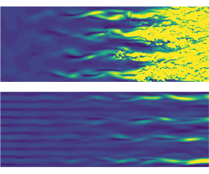
Figure 8 shows contours of instantaneous  $(\rho u)'$ for cases ObSub and ObSubC. Only half the simulation domain in the $z$-direction is displayed since the flow field is symmetric along $z=0$. For the uncontrolled case, the sinuous streak-instability structures appear at $8\times 10^5 < Re_{x} < 10\times 10^5$, indicating that the oblique breakdown mechanism still dominates this scenario. Compared with the pure oblique breakdown (Sharma et al. (Reference Sharma, Shadloo, Hadjadj and Kloker2019), case Cref, figure 4a), the steady vortex mode is now modulated by the subharmonic mode $(1/2,7/4)$. As shown in figure 8(a), the streaky structures are not evenly pronounced and turbulent spots emerge at different positions and time instances on each streak. When the control streaks are applied, the turbulent region is completely shifted out of the considered domain, see figure 8(b).

Figure 8. Instantaneous disturbance  $(\rho u)'$ at $y=0.5$ for cases ObSub (a) and ObSubC (b). Not to scale.
To investigate the role of the MFD (0,0), case ObSubC $_{D}$ is calculated with the disturbance formulation using only the MFD for control. As shown in figure 9(a), the effect of the MFD on the fundamental modes is virtually the same as for the validation case ObC $_{D}$ when including subharmonic modes. Similar as for $(1,1)$, the initial amplitude of the forced subharmonic mode $(1/2,3/4)$ increases when forcing only the MFD, see figure 9(b). However, the amplification of this mode is roughly the same for both cases, even directly downstream of the disturbance input. As discussed above for the validation case ObC $_{D}$, the initially higher growth rate of $(1,1)$ is likely due to streak-induced secondary instability. The behaviour of $(1/2,3/4)$ agrees with the results from the preliminary study by Kneer (Reference Kneer2020), where it is shown that unsteady disturbances with $h < 1$ are less affected by the localized (0,5)-instability. Consequently, the nonlinearly generated mode $(1/2,7/4)$ grows stronger for the MFD-only case, holding also for higher-wavenumber subharmonics. Farther downstream the damping effect of the MFD disappears as the amplitude of $(0,0)$ falls to $1\,\%$. In contrast, if the spanwise modulation by the control streaks is present, the growth of unsteady modes, especially those with relatively high wavenumbers, are more strongly suppressed, since the spanwise traverse of travelling waves is hindered by the streaks.

Figure 9. Streamwise evolution of maximum modal disturbance amplitudes for cases ObSubC and ObSubC $_{D}$ (red, symbols) for fundamental (a) and subharmonic (b) modes. Vertical lines: control strip ( $Re_x\approx 1.6\times 10^5$) and disturbance strip ( $Re_x\approx 2.6\times 10^5$) centres.
5.2. Effect of the control amplitude
Two further cases, ObSubC05 and ObSubC20, with half and twice the control amplitude of ObSubC, respectively, are investigated, see figure 10. While halving the amplitude leads about to the uncontrolled case, doubling it leads to a considerable decrease in disturbance amplitudes. In Sharma et al. (Reference Sharma, Shadloo, Hadjadj and Kloker2019) it is stated that, by choosing a control amplitude that is too large ( ${>}25\,\%$), transition is promoted. For case ObSubC20 this value is surpassed without inducing sudden transition; the value arguably depends on the background noise level, and the present DNS code has a lower one.

Figure 10. Streamwise evolution of maximum modal disturbance amplitudes for cases ObSubC, ObSubC05 (red, gradients) and ObSubC20 (blue, squares). Vertical lines: control strip ( $Re_x\approx 1.6\times 10^5$) and disturbance strip ( $Re_x\approx 2.6\times 10^5$) centres.
6. Flow control for point-source disturbance initiated breakdown
The multi-frequency point source as described in § 2.3.2 is now employed to examine the effectiveness of the control approach for a more complex transition scenario. Due to the highly localized nature of the point source, a full spectrum of oblique disturbance waves is excited. To allow for a disturbance development over a longer downstream distance and to include a wider spanwise wavenumber spectrum, the computation domain W with four times the streamwise and spanwise extent of domain T is used, cf. table 2. Because of the spanwise periodicity it mimics a spanwise row of discrete point sources with a larger spacing now. Thus, disturbance modes with  $k=n/4,\ n \in \mathbb {N}$ can be excited. The time signal of the point source has the form of a large-amplitude pulse consisting of cosine waves with frequencies $h\in \{1/4,\ldots,8/4\}$, each with an amplitude of $A=0.002$. Thus, the unstable frequency band according to the LST throughout the domain can be well covered.
6.1. Point-source-disturbance preliminaries
For the reference case Pt, the control strip is deactivated. The point-source-induced  $(\rho u)'$ spectrum directly downstream of the disturbance input is shown in figure 11. For the directly forced frequencies $h\in \{1/4,\ldots,8/4\}$, the two-dimensional part $k=0$ has approximately half the amplitude of the oblique mode with $k=1/4$, due to the latter being the sum of a counter pair $\pm k$. The amplitude of the oblique modes generally tends to decrease from $k=1/4$ to $k=20$. Since the peak value of the point source is relatively large, disturbances with $h=0$ and $h=9/4$ are also present due to nonlinear generation. Their amplitude, however, is significantly lower than that of the generating modes with $h\in \{1/4,\ldots,8/4\}$.

Figure 11. Disturbance amplitude of induced spanwise wavenumbers for case Pt at  $Re_x=2.680\times 10^5$ of $h=0$ (a), $h=1/4$ (b), $h=1/2$ (c), $h=3/4$ (d), $h=1$ (e), $h=5/4$ (f), $h=3/2$ (g), $h=7/4$ (h), $h=2$ (i) and $h=9/4$ (j).
The downstream development of the modal disturbance amplitudes is shown in figure 12. First, the most amplified modes for each considered input frequency according to the LST are collected in figure 12(a). For  $h>1/2$, these are indeed the modes with the highest amplitude until the onset of transition. It can be observed that the modes with higher frequencies are gradually overtaken by those with lower frequencies since the latter are amplified for a longer distance, as predicted by the LST. We note that the modes that are close in wavenumber to the most amplified mode in the linear stage, as for example $(3/2,1)$, exhibit similar growth rates and amplitudes (not shown).

Figure 12. Streamwise evolution of maximum modal disturbance amplitudes for case Pt. Vertical line: position of the point source ( $Re_x\approx 2.6\times 10^5$). (a) Primary growth of the most unstable oblique waves. (b) Resonant growth of low-frequency disturbances with $h=1/4$ and generation of steady streaks. (c) Tertiary growth prior to the final transition, which is indicated by the saturation of the mean-flow distortion $(0,0)$.
In fact, the existence of the wide  $h$ and $k$ band of amplified modes leads to the growth of various modes with $h=1/4$ as shown in figure 12(b), which are, for the most part, not predicted to be amplified by the LST. The mode $(1/4,7/4)$, for example, is one of the most amplified secondary modes, of which the growth is driven by the asymmetric subharmonic combination-resonance mechanism as discussed in § 3. Since the primarily unstable modes $(1,1)$ and $(3/4,3/4)$ form a resonance triad with $(1/4,7/4)$, the growth of the latter occurs almost immediately downstream of the point source, as the amplitudes of the generating modes are still very small. Although also the mode $(1/4,1/4)$ can be nonlinearly generated by $(1,1)$ and $(3/4,3/4)$, its growth rate in the early stage is significantly lower than that of $(1/4,7/4)$, see figure 12(c). Since the combination-resonance condition (3.2a–c) for the streamwise wavenumbers $\alpha _r$ is mismatched for $(1/4,1/4)$, resonant growth cannot be activated without a mechanism which requires a nonlinear amplitude of the feeding mode. Note that the growth of each secondary mode can possibly be attributed to several resonance triads with various oblique-wave pairs, feeding the secondary mode at different downstream positions. Similar triads for generated modes with $h=1/2$ can also be found. However, these modes are less strongly amplified than their $h=1/4$ counterparts due to fewer possible generating pairs.
Notably, the classical oblique-type mechanism is also present here but does not play a clearly dominant role for the laminar breakdown. As shown in figure 12(b), the steady streak mode  $(0,3/2)$ undergoes a strong amplification prior to breakdown, which is driven by the oblique-wave pairs, e.g. $(3/4,\pm 3/4)$ and $(1/2,\pm 3/4)$. Similarly, $(3/4,\pm 1/2)$ and $(1/2,\pm 1/2)$ serve to feed $(0,1)$. Following the secondary subharmonic mode $(1/4,7/4)$, the steady streak mode $(0,3/2)$ exceeds an amplitude of 1 % at $Re_x\approx 2.4\times 10^6$, together with a number of other modes with $h=1/4$. The nonlinear interaction between them triggers a rapid tertiary growth of the modes $(1/4,1/4)$, $(1/4,1/2)$ and $(0,1/4)$, see figure 12(c). At $Re_x\approx 3.6\times 10^6$, the steady streak mode $(0,1/4)$ grows to an amplitude of 20 %, leading up to the point of transition. The growth is not attributable to any oblique-type mechanism. Instead, this mode is likely generated by the plethora of modes with $h=1/4$. Since these appear strongly in $k=1/4$ increments, all of these modes can generate $(0,1/4)$ with their neighbouring modes in the $k$-spectrum.
In figure 13, the spatial evolution of the wave packet is visualized by showing the instantaneous disturbance velocity  $u'$-contours in physical space at $y=0.38\delta _{99}(x)$ of the base flow. To clearly display the interaction of disturbances generated by two neighbouring point sources, the results are shown over two domain widths. Slightly downstream of the point source, the wave packet mainly consists of oblique waves with relatively high frequencies, which are strongly amplified in the linear stage. At $Re_x\approx 5.0\times 10^5$, it reveals a very similar shape as that observed by Mayer, Laible & Fasel (Reference Mayer, Laible and Fasel2011a), who investigated wave packets in a Mach 3.5 cone boundary layer, where an isolated, one-time-pulsing point source was employed. In contrast, the spanwise periodical and timewise continuous forcing in this study leads to a strong interaction of wave packets as they spread rapidly in streamwise and spanwise direction. Due to the growth of the boundary layer with the connected decreasing streamwise and spanwise wavenumbers of amplified modes, the $\varLambda$-shaped main structures get thicker downstream. In the weakly nonlinear stage, the spanwise modulation of these structures in the front part of the wave packet, as can be seen at $Re_x\approx 1.0\times 10^6$, indicates the subharmonic resonance growth of the $h=1/4$ modes with higher spanwise wavenumbers. At the same time, streamwise elongated streaky structures emerge near the centreline of the wave packets due to the constructive interference of the steady modes generated by the classical oblique-type mechanism. Farther downstream, the $\varLambda$-shaped structures of the linear wave trains completely disappear, and the flow field is dominated by superposed travelling waves with high obliqueness, as shown in the left half of figure 13(b). Eventually, a persistent streak arises at the interface between neighbouring wave trains, respectively domains, prompting the development of turbulent spots. It corresponds to the upshooting of the steady mode $(0,1/4)$ and the rapid growth of all spectral components prior to the final breakdown, see figure 12.

Figure 13. Instantaneous streamwise velocity disturbance  $u'$ at $y=0.38\delta _{99,{baseflow}}$ for case Pt. Logarithmic scales are used for positive values ( $10^{-6}$ to $10^{-1}$) and negative values ( $-10^{-1}$ to $-10^{-6}$) separately; (b) is the spatial continuation of (a). To scale.
6.2. Control mode application
Now, the control mode  $(0,5)$ is forced in case PtC, see figure 14. The suppressing effect of narrowly spaced streaks on the growth of the linearly most amplified modes is shown in figure 14(a). In the previous case Pt without control, the amplification of the modes with $h \geq 1/2$ begins immediately downstream of the point source. With control streaks these modes undergo a transient decay before the unstable eigenmodes exhibit an exponential growth, hence the disturbance receptivity to the point source is attenuated. In addition, the growth rate is diminished, and the unstable region shrinks for each mode. The stabilizing effect is particularly strong for the modes with higher frequency, which are amplified further upstream. This is likely due to the continuous decay of the control mode $(0,5)$ and the MFD $(0,0)$ generated by it. It was hypothesized above that the control mode, and most importantly its three-dimensional structures, have a crucial dampening influence on modes with high wavenumbers, or rather high obliqueness angles. Indeed, for frequency $h=1/2$ the previously most amplified mode $(1/2,3/4)$ is less amplified than $(1/2,1/2)$, when applying the control mode.

Figure 14. Streamwise evolution of maximum modal disturbance amplitudes for cases Pt and PtC (red, symbols). Vertical lines: control strip ( $Re_x\approx 1.6\times 10^5$) and disturbance strip ( $Re_x\approx 2.6\times 10^5$) centres.
As a consequence of the attenuated primary growth, the modes with  $h=1/4$ and $h=0$ that are generated by the subharmonic combination resonance and the oblique mechanism, respectively, decrease in amplitude if compared with the reference case Pt without control, see figure 14(a). The mode $(1/4,1)$, generated mainly by $(1/4,1/2)$ and $(1/2,1/2)$, is one of the most dominant secondary modes and exhibits a larger disturbance amplitude than its feeding mode $(1/4,1/2)$. Furthermore, the steady mode $(0,1)$ is generated by the primary modes $(1/4,1/2)$ or $(1/2,1/2)$ through the classical oblique-type mechanism, eventually surpassing the amplitude of $(1/4,1)$. Compared with case Pt, the spanwise wavenumbers of the dominating secondary modes are lower. This is because the modes with relatively high wavenumber can, in the beginning, only be generated by high-frequency modes, since these are the only ones exhibiting relatively high wavenumbers themselves. Since the modes with $h=1/4$ and $h=0$ are now greatly diminished, their ability to generate tertiary modes, e.g. $(0,1/4)$, is in turn also reduced.
Figure 15 shows how the growth of wave trains is attenuated by the narrowly spaced control streaks in physical space. Oblique-wave structures are only visible at  $Re_x\approx 1.6\times 10^6$. Turbulent spots are not observed within the computation domain. To quantify the drag reduction, the skin-friction-coefficient distribution for both cases is compared in figure 16. For the controlled case PtC, a narrow local increase of $c_f$ is visible at the blowing-and-suction strip. However, it quickly decays to the value of the uncontrolled case Pt. The increase of $c_f$ for case Pt at $3.2\times 10^6 \leq {Re}_x \leq 4.0\times 10^6$ indicates the laminar breakdown. For the controlled case PtC transition to turbulence does not occur in the considered domain, and the skin friction remains on the low laminar level.

Figure 15. Instantaneous streamwise velocity disturbance  $u'$ at $y=0.38\delta _{99,{baseflow}}$ for case PtC. Logarithmic scales are used for positive values ( $10^{-6}$ to $10^{-1}$) and negative values ( $-10^{-1}$ to $-10^{-6}$) separately; (b) is the spatial continuation of (a). To scale.

Figure 16. Downstream development of the skin-friction coefficient  $c_f$ for cases Pt and PtC.
Conclusively, the application of the control mode  $(0,5)$ to this scenario is highly beneficial. The transition location can be shifted significantly downstream by diminishing the disturbance receptivity and linear amplification of the forced disturbance modes, especially the high-frequency modes. Thus, fewer resonance triads can be formed, and any combination-resonance growth is attenuated due to the lowered primary growth rate of the feeding modes. The downstream development of the secondary and tertiary modes is greatly influenced even after the control mode has decayed to an irrelevant level, because the scenario has been deprived of a large number of otherwise relevant disturbance modes.
7. Roughness-induced control streaks
To further investigate the applicability of control streaks in a supersonic boundary layer, an effort was made to introduce such modes using distributed roughness elements. The considered roughness configuration consists of a spanwise row of smoothly shaped surface bumps as described in § 2.3.4. Similar roughness configurations in supersonic boundary-layer flow were investigated in the past, but only with focus on either roughness-induced transition, see for example Muppidi & Mahesh (Reference Muppidi and Mahesh2012) and Choudhari et al. (Reference Choudhari, Li, Paredes and Duan2019), or turbulent flow, see, e.g. Ekoto et al. (Reference Ekoto, Bowersox, Beutner and Goss2008). In this section we first analyse the generation and downstream development of the roughness-induced streaks in comparison with those excited by the blowing-and-suction strip. The control performance and the effect of the roughness height are then discussed.
7.1. Streak generation
To compare the streak excitation by distributed roughness elements and blowing and suction, simulations are conducted in a short integration domain R without additional disturbance input, cf. table 3. For case C the same blowing-and-suction amplitude as for case ObC, i.e. the reference case to Sharma et al. (Reference Sharma, Shadloo, Hadjadj and Kloker2019), is used. For case R8 the roughness height  $H=0.8$, corresponding to approximately $60\,\%\cdot \delta _{99}$ locally, is chosen such that the excited control mode $(0,5)$ reaches the same amplitude at $Re_x\approx 2.7\times 10^5$, which is the location of the disturbance-input strip (inactive here). The time-resolved computations converge to a steady state, indicating the global stability of the flow configuration.
The downstream development of the control mode  $(0,5)$ for both cases is compared in figure 17. Although the amplitude of $(0,5)$ immediately downstream of the roughness elements is relatively low, it increases to roughly the same as that for case C at $Re_x\approx 2.7\times 10^5$. It is still increasing up to $Re_x\approx 3.5\times 10^5$, whereas it is constantly decreasing for case C. Further downstream, the damping rate of the intended control mode is considerably lower for the roughness case when compared with blowing and suction, promising better flow-control capabilities. Similar to case C, the MFD $(0,0)$ for case R8 decays continuously after being excited, and its decay rate asymptotes to that of the streak mode $(0,5)$. The weak oscillation of $(0,0)$ is likely due to the interference between the compression and expansion waves formed at the windward and leeward edges of the roughness elements, respectively. Since they have a smooth shape, the pressure waves downstream of the elements are infinitesimal, and thus negligible compared with the streak-induced flow deformation.

Figure 17. Streamwise evolution of modal amplitudes for cases C and R8 (red, gradients). Vertical lines: start of roughness ( $Re_x\approx 1.5\times 10^5$), end of roughness ( $Re_x\approx 1.7\times 10^5$) and disturbance strip centre (inactive, $Re_x\approx 2.6\times 10^5$).
For a better understanding of the streak-generation process and the underlying flow topology, the wall-pressure distribution and skin-friction lines in the vicinity of a roughness element are presented in figure 18. On the centreline of the peak, the flow is compressed near the bump leading edge and then expanded on the top side. On the leeward side, a separation bubble emerges due to the adverse pressure gradient. On the centreline of the valley, the streamwise variation of the wall pressure is qualitatively the same but much weaker. The resulting spanwise pressure gradient drives the near-wall fluid around the bump element and then towards the recirculation zone. Due to the downward fluid motion and the pressure increase in the later reattachment region, the limiting streamlines are finally redirected slightly towards the centreline of the valley, i.e. to the line between the bumps.

Figure 18. Surface-pressure distribution and skin-friction lines in the vicinity of a roughness element in case R8. Perspective view, the top line is the centreline of the element.
Figure 19(a) shows the induced vortical motion in a cross-cut at  $x=100$ ( $Re_x\approx 1.9\times 10^5$). In the near-wall region, a cross-flow towards the valley centreline $z=2.7$ is driven by the spanwise pressure gradient. The high-inertia flow farther away from the wall, however, retains the history of the upstream pressure gradient which pushed the flow towards the recirculation zone. The spanwise convection, together with the downward reattachment flow, promotes a pair of counter-rotating vortices, which correspond to the largest streamwise vorticity concentrations that also represent the trailing legs of a horseshoe vortex around the element in figure 19(a). The resulting lift-up effect contributes to the formation of the low-speed streak (LSS) in the wall-normal plane between the bumps, see figure 19(b). Meanwhile, another but weaker pair of vorticity concentrations can be identified. They initially develop above the recirculation zone in the bump peak plane, supported by the cross-flow coming around the lateral edges towards the peak centreline. However, these vorticity concentrations decay rapidly downstream of the separation bubble as the driving force fades out. Also the LSS on the peak centreline, left over from the recirculation, tends to fade away since the vorticity concentrations are not able to generate sufficient lift-up effect from the near-wall region. Note that the relative importance of the two vortex systems described and thus the spanwise position of the LSS generally depends on the element's shape. Here, the length of the elements is approximately twice the width, and the legs of the horseshoe vortex dominate (as for needle-type roughness elements), not the recirculation-zone (inner) vortex pair. Direct flow tripping by global instability is thus shifted to relatively large critical roughness Reynolds numbers $Re_{kk, {crit}}$. For case R8, $Re_{kk}=682$ taking the velocity and kinematic viscosity at the roughness height of the base flow, or $448$ with the viscosity at the wall. For broad, sharp-edged roughness elements with aspect ratio one these values may be close to the global-instability limit in the supersonic flow, but with the thin, smooth, longer-than-wide elements applied here the critical value is significantly higher and no onset of global instability has been observed.

Figure 19. Cross-cuts at  $x=100$ ( $Re_x=1.9\times 10^5$). Contours of streamwise vorticity $\omega _x$ and $(v,w)$-velocity vectors for cases R8 (a) and C (c). Contours of velocity gradient $\partial u/\partial z$ and $u$-isolines for cases R8 (b) and C (d).
For comparison, the corresponding cross-cuts for case C are displayed in figures 19(c) and 19(d), respectively. Note that the LSS planes  $z$=const. between the bumps correspond to the positions of strongest blowing of the blowing-and-suction strip. The main vorticity concentrations show a similar spatial distribution as for case R8, whereas the other vorticity concentrations from before are absent since flow separation does not occur for the blowing-and-suction case. A LSS with local boundary-layer thickening is visible at $z=2.7$, directly downstream of the local wall-normal blowing. A second LSS cannot be found at $z=0$. Instead, a clear high-speed streak (HSS) directly arises from the wall-normal suction. Farther downstream at $x=150$ ( $Re_x\approx 2.9\times 10^5$), see figure 20, the streamwise vorticity decays significantly for both cases and exhibits roughly the same pattern. Compared with figure 19(b), the velocity isocontours for the roughness case in figure 20(b) shows that the LSS on the valley centreline becomes more pronounced due to the transient growth supported by the counter-rotating streamwise vortex pair, whereas the LSS on the peak centreline dies out as expected. Consequently, a changeover in spanwise phase of the steady $(\rho u)'$ disturbance mode $(0,5)$ takes place, which is reflected in the V-shaped amplitude development of $(0,5)$ and the high level of $(0,10)$ downstream of the roughness elements in figure 17. The boundary-layer deformation shown in figure 20(d) for the blowing-and-suction generation appears very similar. The LSS results directly from local wall blowing. Comparing with the cross-cut at $x=100$, the boundary-layer thickening becomes more localized and the streak amplitude is smaller, which is indicated by the reduced maximum of $\partial u/\partial z$.

Figure 20. Cross-cuts at  $x=150$ ( $Re_x=2.9\times 10^5$). Contours of streamwise vorticity $\omega _x$ and $(v,w)$-velocity vectors for cases R8 (a) and C (c). Contours of velocity gradient $\partial u/\partial z$ and $u$-isolines for cases R8 (b) and C (d).
It seems that with blowing and suction, locally a more relaxed spatial distribution of the longitudinal vorticity and ensuing streaky structures is achieved. (We note that accounting for blowing and suction channels the velocity distribution at the wall within the control strip may differ somewhat from the modelled one; but with the relatively small blowing ratio of approximately 2.5 % the difference is not expected to be significant.) In other words, the generated streaks are not able to gain more disturbance energy through a transient growth mechanism despite the existence of a counter-rotating streamwise vortex pair. In the roughness case, the initial condition of  $u'$ does not fit in with the streamwise vortices. Therefore, a transient, relaxing, re-shaping process takes place to the streaky structures. Thus, the maximum of the steady streak mode is reached later, and the decay also. At the latter downstream positions, a specific ‘natural’ state of boundary-layer deformation with the given spanwise wavenumber is reached, which is virtually the same as that generated by blowing and suction. The decay rate of the streak, however, is sensitive to the initial condition because of the nonlinearity of the streak behaviour. A similar nonlinearity was observed by Paredes, Choudhari & Li (Reference Paredes, Choudhari and Li2016), when considering the decay of large-amplitude steady streaks, which experienced optimal transient growth with different initial conditions in a supersonic boundary layer.
7.2. Full flow development
Case ObR8 has been performed in order to generate results comparable to case ObC. The same roughness shape from case R8 and the full-length integration domain T is used. Since the applicability of the control mode  $(0,5)$ to a complex scenario has successfully been verified, we only excite the mode $(1,1)$ using the disturbance strip to investigate the effect of roughness-element-induced control streaks.
It is apparent from figure 21 that the initial, transiently growing nature of the control streaks in the roughness case leads to an increased flow-control capability, when compared with the blowing-and-suction case. While the maximum amplitude of  $(0,5)$ is about the same for both cases, it is reached at a far later position for case ObR8 and decays at a much lower rate. Accordingly, $(0,0)$ decays also at a much lower rate. Consequently, the suppression of all the disturbance modes is also stronger.

Figure 21. Streamwise evolution of maximum modal disturbance amplitudes for cases ObC and ObR8 (red, symbols). Vertical lines: start of roughness ( $Re_x\approx 1.5\times 10^5$), end of roughness ( $Re_x\approx 1.7\times 10^5$) and disturbance strip centre ( $Re_x\approx 2.6\times 10^5$).
7.3. Effect of roughness height
To investigate the effect of the roughness height on the control capabilities three more cases, ObR6, ObR7 and ObR9, with heights of  $H\in \{0.6,0.7,0.9\}$ were run.
The downstream development of disturbance modes for these cases can be seen in figure 22. As expected, varying the roughness height has similar effects as varying the blowing-and-suction forcing amplitude. With the strong damping of  $(1,1)$, the amplitudes of modes $(1,3)$ and $(1,5)$ are consequently also damped for all cases employing a roughness array, with the exception of case ObR6. Since the mode $(0,2)$ has a rather large amplitude when $(1,1)$ starts getting damped, the former's growth is largely unaffected by that phenomenon. For case ObR9, the downstream development of $(1,5)$ is distinctly different. Initially, the disturbance amplitude is magnitudes higher, but, further downstream, the mode is far less amplified. It is likely that the unsteady modes are locally amplified in the near-wake region behind the highest roughness elements. However, the amplification does not seem to be critical since it is spatially restricted and compensated by the beneficial effect of the control streaks.

Figure 22. Streamwise evolution of maximum modal disturbance amplitudes for cases ObR6, ObR7 (red, deltas), ObR8 (blue, gradients) and ObR9 (green, squares). Vertical lines: start of roughness ( $Re_x\approx 1.5\times 10^5$), end of roughness ( $Re_x\approx 1.7\times 10^5$) and disturbance strip centre ( $Re_x\approx 2.6\times 10^5$).
The modal amplitude development that most closely fits that of the blowing-and-suction case is that for case ObR7. When plotting both side by side, see figure 23, it can be seen that most disturbance modes show a similar evolution for long downstream distances. Until  $Re_x\approx 7\times 10^5$, the development of all modes but $(0,5)$ look very similar. This indicates that the MFD plays an important role in the early stages of the control. The role of $(0,5)$ must therefore be negligible, since the similar downstream development could not be explained otherwise. However, in the roughness case, the mode $(1,1)$ is continuously damped for positions downstream of $Re_x\approx 8\times 10^5$, whereas it grows again at the end of the domain for the blowing-and-suction case. This is in line with the results from above. Once the oblique travelling modes, i.e. $(1,1)$, $(1,3)$ and $(1,5)$, reach significant amplitudes, the role of the three-dimensional structures becomes more and more important. Due to the higher amplitude of the control mode $(0,5)$ in the roughness case, these are obviously more pronounced and can therefore be more effective at suppressing these oblique modes.

Figure 23. Streamwise evolution of maximum modal disturbance amplitudes for cases ObC and ObR7 (red, symbols). Vertical lines: start of roughness ( $Re_x\approx 1.5\times 10^5$), end of roughness ( $Re_x\approx 1.7\times 10^5$) and disturbance strip centre ( $Re_x\approx 2.6\times 10^5$).
8. Conclusions
Building on results by Sharma et al. (Reference Sharma, Shadloo, Hadjadj and Kloker2019), the effectiveness of narrowly spaced streaks in delaying laminar-to-turbulent transition in a boundary layer at  $M_{\infty }=2.0$ has been investigated. Streaks with five times the wavenumber of the fundamental oblique breakdown mode $(1,1)$, i.e. $(0,5)$, have been introduced using either blowing and suction or surface roughness elements to control the breakdown in various scenarios.
For the first of these scenarios/mechanisms, i.e. pure oblique breakdown, results have already been reported by Sharma et al. (Reference Sharma, Shadloo, Hadjadj and Kloker2019) and could be fully verified. Regarding the role of the mean-flow distortion (MFD), the use of a true disturbance formulation enabled to gain an important insight into the damping caused by the forced control streaks. The MFD is not consistently able to suppress the growth of high spanwise wavenumber combination modes, e.g.  $(1,5)$, hinting at the importance of the three-dimensional control part after the decay of the MFD.
The control technique is also effective when a typical (asymmetric) subharmonic combination-resonance triad is present. Disturbance formulation simulations employing only the MFD as control revealed that the three-dimensional structures of the control play a somewhat more important role in this scenario. This is most likely due to the combination modes  $(1/2,3/4)$ and $(1/2,7/4)$ having a higher obliqueness angle than $(1,1)$, rendering those less sensitive to the MFD without the three-dimensional control component.
In order to investigate the scenario with a more realistic transition Reynolds number and involving a wider disturbance spectrum, a multi-frequency point source has been employed in a wider and longer integration domain. A highly complex scenario characterized by multiple subharmonic combination resonances and considerable wave train component interactions emerges. The control by streaks turns out to be effective also in this scenario by damping the primary growth of the disturbances greatly and thus reducing their capabilities to nonlinearly feed the subharmonic secondary modes.
The control streaks can be also forced by roughness elements that are here smooth and twice as long as wide. Compared with the generation by blowing and suction, i.e. wall-normal velocity forcing, the roughness-induced three-dimensional deformation of the boundary layer exhibits a less relaxed state. The  $z={\rm const}$. planes with relevant updraft, eventually forming the low-speed streaks, change rapidly in the near wake of the bumps, from the bump peak positions to the lines between the bumps. Consequently the streaks undergo a transient growth by this re-shaping process, reach their maximum amplitude farther downstream, and decay slower. Thus the roughness elements show an enhanced control performance since the desired streak modes and the MFD persist for longer downstream distances. However, in an effort to maximize the control-streak amplitude the flow appears more sensitive to elements too high compared with high blowing-and-suction amplitudes.
Funding
Computational resources have been provided by the Gauss Centre for Supercomputing (grant GCS-Lamt, ID = 44026) on the national supercomputers Cray XC40 and HPE Apollo at the Federal High Performance Computing Center Stuttgart (HLRS). The work was supported by the China Scholarship Council (Z.G., grant 201708080155).
Declaration of interests
The authors report no conflict of interest.


 Open access