


1. Introduction
Hydraulic jumps are among the most iconic phenomena in fluid dynamics, found in a variety of situations ranging from thin films and kitchen sinks to large-scale open channels. They mark the sudden transition from a fast, relatively thin supercritical flow to a slower and thicker subcritical one (see figure 1). The systematic study of hydraulic jumps was initiated in the first half of the 19th century by the experiments of Bidone and the theoretical investigations of Bélanger (Bakhmeteff Reference Bakhmeteff1932; Chanson Reference Chanson2009). The latter established the textbook explanation of the phenomenon, based on conservation of mass and momentum, ignoring any additional effects such as the slope of the channel, the friction with the bottom (arising from shear stresses in the flow), diffusive effects (due to in-plane stresses) or surface tension. Only during the past few decades have these effects begun to be incorporated, often via approaches that depart from that of Bélanger (Bowles & Smith Reference Bowles and Smith1992; Bohr, Dimon & Putkaradze Reference Bohr, Dimon and Putkaradze1993; Higuera Reference Higuera1994; Bohr, Putkaradze & Watanabe Reference Bohr, Putkaradze and Watanabe1997; Ruschak & Weinstein Reference Ruschak and Weinstein2001; Watanabe, Putkaradze & Bohr Reference Watanabe, Putkaradze and Bohr2003; Bonn, Andersen & Bohr Reference Bonn, Andersen and Bohr2009; Rojas et al. Reference Rojas, Argentina, Cedra and Tirapegui2010; De Vita et al. Reference De Vita, Lagrée, Chibbaro and Popinet2020).

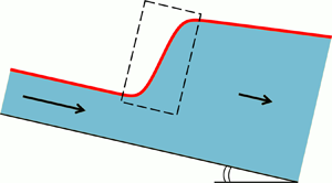
Figure 1. Schematic view of a stationary hydraulic jump in a tilted channel, i.e. the transition zone of length  $L$ from a shallow supercritical flow (Froude number
  $F>1$) to a thicker subcritical one (
 $F<1$), where
  $F = \bar {u}(x)/\sqrt {gh(x) \cos \zeta }$. The flow is described in terms of the height
  $h(x)$ and the depth-averaged velocity
  $\bar {u}(x)$, governed by the generalized Saint-Venant equations (2.2) and (2.3). The depicted jump corresponds to the profile
  $\tilde {M}3 \rightarrow \tilde {M}2$ of figure 2(a), which is one of the four qualitatively different types of laminar jumps predicted by our analysis, cf. figure 3.
Without the inclusion of higher-order effects such as the in-plane stresses or surface tension, the supercritical and subcritical flow regimes do not connect continuously but have to be linked to each other via vertical segments obeying the Rankine–Hugoniot shock relations (Rayleigh Reference Rayleigh1914; Whitham Reference Whitham1974; Landau & Lifschitz Reference Landau and Lifschitz1987; Mejean, Faug & Einav Reference Mejean, Faug and Einav2017; Castro-Orgaz & Hager Reference Castro-Orgaz and Hager2019; Dhar, Das & Das Reference Dhar, Das and Das2019). A drawback of this approach is that the internal structure of the jump remains unaccounted for. Pioneering studies to reveal this structure have used either a boundary layer analysis to the governing Navier–Stokes equations (Bohr et al. Reference Bohr, Putkaradze and Watanabe1997; Ruschak & Weinstein Reference Ruschak and Weinstein2001; Watanabe et al. Reference Watanabe, Putkaradze and Bohr2003; Bonn et al. Reference Bonn, Andersen and Bohr2009) or a perturbation expansion of those equations leading to the lubrication approximation for the circular jump (Rojas et al. Reference Rojas, Argentina, Cedra and Tirapegui2010). Here we deal with this problem from the standpoint of hydraulics, by analysing the generalized Saint-Venant equations (Needham & Merkin Reference Needham and Merkin1984; Merkin & Needham Reference Merkin and Needham1986; Kranenburg Reference Kranenburg1992; Castro-Orgaz & Hager Reference Castro-Orgaz and Hager2019) which are tailor-made for laminar channel flow and enable us to derive an approximate analytic expression for the jump length  $L$.
$L$.
The forces governing the shape of the hydraulic jump are gravity, surface tension and viscous forces. Just as for usual surface waves, gravity is dominant at large scales while surface tension becomes important at small scales. Surface tension and viscosity (especially the in-plane stresses) are instrumental in preventing the development of discontinuities, by keeping the slope of the fluid profile always finite. These effects come into play in the flow regions where the height and velocity change rapidly.
The familiar jump in the kitchen sink is on the relatively small scale where gravity, surface tension and viscosity all contribute, and is therefore, despite its everyday occurrence, a surprisingly intricate case (Bhagat et al. Reference Bhagat, Jha, Linden and Wilson2018; Duchesne, Andersen & Bohr Reference Duchesne, Andersen and Bohr2019). On the largest scale, one finds the fully developed turbulent jumps of spillways and rapids, where gravity takes the undisputed lead. The present paper deals with jumps on the intermediate scale where surface tension becomes insignificant, leaving gravitational and viscous effects as the two main factors. Such jumps may be encountered in irrigation ditches or tilted channels on the laboratory scale under laminar or moderately turbulent flow conditions. The fluid in question may be taken to be water, but the description will become increasingly accurate if one uses a Newtonian fluid with a higher viscosity and lower surface tension, e.g. silicon oil or castor oil. The Reynolds number can then be kept effortlessly at the moderate levels of laminar or just-turbulent flow, while the surface tension – already very minor at this scale – can safely be ignored. As for the Froude number  $F$ of the incoming flow, this must naturally exceed
  $1$ yet it should remain bounded within the realm of what is traditionally known as a ‘weak jump’ (Chow Reference Chow1973). For
  $1 < F \lesssim 1.7$ the rise in surface level is limited and the energy dissipation is less than
  $5\,\%$. Around
  $F \sim 1.7$, small rollers develop on the surface of the jump, yet farther downstream the profile remains smooth and the velocity fairly uniform, with relatively small energy losses (5–15 %). This state of affairs persists up to
  $F \sim 2.5$, and this value marks the border of the regime where the jump may be called weak. For
  $F > 2.5$ one finds fiercer jumps, which fall outside the scope of the present study (Çengel & Cimbala Reference Çengel and Cimbala2006; Munson et al. Reference Munson, Young, Okiishi and Huebsch2009).
The paper is organized as follows. In § 2 we present the generalized Saint-Venant equations for shallow channel flow, including a diffusive term accounting for the in-plane stresses, and from these we derive a second-order ordinary differential equation (ODE) governing the stationary wave profiles that are possible within this framework. This constitutes an extension of the classical first-order ‘backwater equation’ used to describe gradually varied flow (Rouse Reference Rouse1946). In § 3 we cast the aforementioned second-order ODE in the form of a dynamical system consisting of two coupled first-order ODEs, and analyse its phase space. Here the hydraulic jumps appear as conspicuous quasi-parabolic orbits linking the nullclines of the dynamical system. The steep excursion in phase space corresponds to the pronounced rise in the slope of the fluid profile locally across the jump, whereas the nullclines represent the diffusive counterparts of the classical gradually varied profiles at either side of the jump. In § 4 we concentrate on the jump region and derive an analytic approximation for its spatial extent along the channel, i.e. the jump length  $L$. In § 5 we return to the generalized Saint-Venant equations and study the temporal evolution of small perturbations imposed upon the jump profiles. The observed decay of these perturbations confirms the stability of the jump. Finally, § 6 summarizes the main findings of this study.
2. The governing equations
2.1. The generalized Saint-Venant equations
For the description of the fluid sheet we adopt the one-dimensional framework of the so-called shallow-water flow. This one-dimensional description does not account for the velocity component in the vertical direction (which obviously must exist in the jump region, since the fluid has to rise to a larger height here), nor does it capture any motion in the crosswise direction (so secondary flow patterns induced by the interaction of the fluid with the sidewalls are ignored). In the shallow-water approach, the flow in the channel is described solely by the height  $h(x,t)$ of the fluid sheet and its depth-averaged velocity
  $\bar {u}(x,t)$, defined as follows:
 \begin{equation} \bar u (x,t) = \frac{1}{h(x,t)} \int_{0}^{h(x,t)} u(x,z,t)\,\textrm{d} z, \end{equation}
where  $u(x,z,t)$ is the detailed velocity profile. For laminar flows, as in the present study, for which the velocity profile does not vary significantly in the bulk of the sheet (outside a narrow boundary layer near the bottom), the above averaging may be expected to give physically plausible results. Our analysis should be considered as a mean field theory, giving the height profile
  $h(x,t)$ without any special effects – such as undulations, surface rolls or eddies – arising from the internal dynamics in the fluid sheet. As such, it is suitable for describing ‘type I’ jumps, i.e. jumps without separation rollers (containing regions of back-flow) along the surface of the flow (Chow Reference Chow1973; Ellegaard et al. Reference Ellegaard, Hansen, Haaning and Bohr1996).
The two quantities  $h(x,t)$ and
  $\bar {u}(x,t)$ are governed by a generalized version of the Saint-Venant equations (Kranenburg Reference Kranenburg1992), i.e. the two coupled partial differential equations (PDEs) expressing, respectively, the mass balance
 \begin{equation} h_t + (h \bar{u})_x = 0 \end{equation}
and the momentum balance
 \begin{equation} (h \bar{u})_t + (h \bar{u}^2)_x = gh \sin \zeta - \left({\tfrac{1}{2}} g h^2\cos \zeta \right)_x - C_f \bar{u}^2 + \nu (h \bar{u}_x)_x . \end{equation}
The terms on the right-hand side of (2.3) represent the various forces acting on the water sheet. In order of appearance they are the following.
(i) The gravity component in the
 $x$-direction, where $g=9.81\ \textrm {m}\ \textrm {s}^{-2}$ is the gravitational acceleration and $\zeta$ the inclination angle of the channel.
(ii) The gradient of the depth-averaged pressure, arising from the variations in
$h(x,t)$, where the pressure within the fluid layer is in leading order taken to be hydrostatic.(iii) The friction with the bottom of the channel arising from the viscous shear stresses, known as Chézy's formula (Needham & Merkin Reference Needham and Merkin1984; Balmforth & Mandre Reference Balmforth and Mandre2004; Fowler Reference Fowler2011). The dimensionless friction factor
$C_f$ depends on the Reynolds number and the roughness of the bottom (Rouse Reference Rouse1946; Kranenburg Reference Kranenburg1992). It is determined by the shear stresses arising from the sharp velocity gradient in the boundary layer at the bottom of the channel, where the velocity drops to zero to comply with the no-slip condition. For laminar flow over a smooth plate – comparable to the channel bed – it is given by the expression $C_f = 0.664\,Re^{-1/2}$ (Rouse Reference Rouse1946), with the Reynolds number $Re$ being typically of the order $10^2\text {--}10^5$. For our purposes, therefore, $C_f$ will be a small parameter of the order 0.002–0.07. Incidentally, the related interval for turbulent flows over relatively rough channel beds ($0.002 < C_f < 0.006$) lies entirely within this range (Kranenburg Reference Kranenburg1992).(iv) The force due to the viscous normal stresses, where
$\nu$ denotes an empirical positive coefficient with the dimensions of a kinematic viscosity. The latter diffusive term was absent from the classical Saint-Venant equations. Several forms, suitable for different flow regimes, have been proposed over the years (see for example Needham & Merkin (Reference Needham and Merkin1984)). The one adopted here was derived by Kranenburg (Reference Kranenburg1992) for laminar and moderately turbulent flows. Typically, since the flow is shallow, the bottom friction is the primary source of dissipation. So we take $\nu$ to be small, and consequently our results do not depend substantially on the precise form of the diffusive term. Finally, as discussed in the introduction, the jumps we are interested in are too large to be noticeably affected by surface tension – therefore, any capillary force terms have been left out of (2.3).


2.2. Stationary wave solutions
The above set of equations has been used successfully to reproduce travelling waveforms in open channel flow, such as roll waves (Needham & Merkin Reference Needham and Merkin1984; Merkin & Needham Reference Merkin and Needham1986; Kranenburg Reference Kranenburg1992; Balmforth & Mandre Reference Balmforth and Mandre2004). Here we employ the same equations to describe a stationary waveform, namely the standing hydraulic jump. In order to capture this type of wave, we seek solutions of the form  $h=h(x)$ and
  $\bar {u}=\bar {u}(x)$. This implies that the derivatives with respect to
  $t$ in (2.2) and (2.3) vanish identically.
The time-independent version of the mass balance (2.2) can readily be integrated, yielding  $h \bar {u} = Q$, where
  $Q$ is the constant flux of water (per unit width) in the channel. Inserting the relation
  $\bar {u}(x) = Q h(x)^{-1}$ into the time-independent version of (2.3), we obtain a second-order ODE for
  $h(x)$ as follows:
 \begin{equation} \frac{\nu}{Q} h h'' = \frac{\nu}{Q} (h')^2 + \left( 1 - \frac{h^3}{h_c^3} \right) h' -C_f \left( 1 - \frac{h^3}{h_n^3} \right), \end{equation}
where the prime stands for differentiation with respect to  $x$, the combination
  $Q/ \nu \equiv R$ is an effective Reynolds number of the flow (since
  $\nu$ is an empirical coefficient with the dimensions of viscosity), while the heights
  $h_c$ and
  $h_n$ are given by
 \begin{equation} h_c = \left( \frac{Q^2}{g \cos \zeta} \right)^{1/3},\quad h_n = \left( \frac{C_f Q^2}{g \sin \zeta} \right)^{1/3}. \end{equation}
In the context of gradually varied flow, these are known as the critical and natural height, respectively (Bakhmeteff Reference Bakhmeteff1932; Rouse Reference Rouse1946). At  $h=h_c$ the Froude number
  $F = \bar {u}/\sqrt {gh \cos \zeta } = Q/\sqrt {gh^3 \cos \zeta } = (h_c/h)^{3/2}$ equals 1, marking the border between supercritical flow (
 $F >1$,
  $h < h_c$) and subcritical flow (
 $F<1$,
  $h>h_c$). The height
  $h_n$ is the water thickness under uniform flow conditions, i.e. with
  $h$ and
  $\bar {u}$ constant, such as may be found in the fully ripened flow far from the inlet and outlet of the chute. The expression for
  $h_n$ follows from (2.3) by setting all derivatives equal to zero, leaving only the forces of gravity and friction to balance each other.
The quotient  $(h_c/h_n)^3 = \tan \zeta / C_f$ forms the basis for the standard classification of channels into two categories (Bakhmeteff Reference Bakhmeteff1932; Rouse Reference Rouse1946; Chow Reference Chow1973; LeMéhauté Reference LeMéhauté1976): (1) those that are hydraulically mild for
  $h_c < h_n$; and (2) those that are hydraulically steep for
  $h_c > h_n$. Equivalently, one might talk about hydraulically ‘rough’ and ‘smooth’ channels, respectively.
2.3. Connection to the classical ‘backwater equation’
Equation (2.4) shows precisely what the inclusion of the diffusive term modelling the in-plane stresses has added to the description of the hydraulic jump, namely, the terms with  $h h''$ and
  $(h')^2$. Indeed, in the non-diffusive limit
  $\nu \rightarrow 0$, (2.4) reduces to the relation that is traditionally used to describe gradually varied flow, known as the ‘backwater equation’ (Chanson Reference Chanson2009),
 \begin{equation} h' = C_f \frac{ 1 - (h/h_n)^3}{1 - (h/h_c)^3} = \tan \zeta \frac{h^3-h_n^3}{h^3-h_c^3}. \end{equation}
 The classical procedure is to derive from this non-diffusive relation the separate flow profiles upstream and downstream of the jump, and to link these together via shock conditions. For mild channels, there are three distinct profiles:  $M1$ (for
  $h>h_n$);
  $M2$ (
 $h_c < h < h_n$); and
  $M3$ (for
  $h < h_c$) (see figure 2a for their diffusive counterparts). Of these three, the profile
  $M_3$ is the only supercritical one, so the jump connects
  $M3$ either to
  $M2$ or to
  $M1$. Also, for steep channels there are three distinct profiles:
  $S1$ (for
  $h>h_c$);
  $S2$ (
 $h_n < h < h_c$); and
  $S3$ (for
  $h < h_n$) (cf. figure 2b). In this case, both
  $S2$ and
  $S3$ are supercritical, hence the jump connects either of these profiles to
  $S1$. Any of these jumps links a region of supercritical flow to a subcritical one, and hence occurs when the level of the water passes through the critical height
  $h_c$. In the non-diffusive expression (2.6), the slope
  $h'$ becomes infinite for
  $h=h_c$, so the jump appears as a discontinuity in the profile
  $h(x)$, i.e. as a vertical segment connecting the supercritical and subcritical regimes. This unphysical feature is remedied, as we will demonstrate, by the inclusion of the second-order term
  $\nu (h \bar {u}_x)_x$. The crux of the matter is that the solutions of the diffusive equation (2.4) cross the height
  $h_c$ with a finite slope.

Figure 2. Phase portraits of the dynamical system (3.1a) and (3.1b) for mild (a) and steep (b) channels, which are seen to be each other's mirror image. The solid red and blue curves represent the two types of hydraulic jumps occurring in each channel. The jump region manifests itself as a near-parabolic orbit. The dashed violet curves are the branches of the nullcline  $\tilde {s}_{\pm }(\tilde {h})$, (3.2), forming the guiding lines for the gradually varied profiles at either side of the jump. (a) Mild: the curves travel together in the supercritical regime, follow the stable manifold (dashed black curve) of the saddle point
  $(\tilde {h}_n,0)$ and afterwards, in the subcritical regime go their separate ways; the associated profiles
  $\tilde {h}(\tilde {x})$ (insets) are the jumps
  $\tilde {M}3 \rightarrow \tilde {M}1$ and
  $\tilde {M}3 \rightarrow \tilde {M}2$. (b) Steep: the curves start out separately in the supercritical regime, follow the unstable manifold of the saddle (black dashed curve) and come together in the subcritical regime; the profiles
  $\tilde {h}(\tilde {x})$ (insets) are the jumps
  $\tilde {S}3 \rightarrow \tilde {S}1$ and
  $\tilde {S}2 \rightarrow \tilde {S}1$. The dotted lines indicate the critical height
  $\tilde {h} = 1$ and the natural height
  $\tilde {h}_n$. The grey arrows in the background show the direction field. Parameters: inclination angle
  $\zeta = 2^\circ$, effective Reynolds number
  $R=20$, with
  $C_f = 0.07$,
  $F_n = 0.7$ (mild) and
  $C_f = 0.02$,
  $F_n = 1.4$ (steep).
At this point we choose to turn to non-dimensional variables, which will be denoted by tildes. We take  $h_c$ as our unit length, so
  $\tilde {x}= x/h_c$ and
  $\tilde {h} = h/h_c$. Equation (2.4) then takes the non-dimensional form
 \begin{equation} \frac{1}{R} \tilde{h} \frac{\textrm{d}^2 \tilde{h}}{\textrm{d} \tilde{x}^2}= \frac{1}{R} \left( \frac{\textrm{d} \tilde{h}}{\textrm{d} \tilde{x}} \right)^2 + \left( 1 - \tilde{h}^3 \right) \frac{\textrm{d} \tilde{h}}{\textrm{d} \tilde{x}} -C_f \left( 1 - F_n^2 \tilde{h}^3 \right), \end{equation}
where  $R \equiv Q/\nu$ is the effective Reynolds number introduced earlier. The Froude number
  $F_n$ is taken at the natural height
  $h_n$, or equivalently, at
  $\tilde {h}_n = h_n/h_c = F_n^{-2/3}$.
3. Dynamical systems approach
3.1. The dynamical system and its fixed point
The second-order ODE equation (2.7) can be cast in the form of a dynamical system consisting of two first-order ODEs, as follows:
 \begin{gather} \frac{\textrm{d} \tilde{h}}{\textrm{d} \tilde{x}} = \tilde{s} \equiv f_1(\tilde{s}), \end{gather}
 \begin{gather}\frac{\textrm{d} \tilde{s}}{\textrm{d} \tilde{x}} = \frac{1}{\tilde{h}} \left(\tilde{s}^2 + R \left( 1 - \tilde{h}^3 \right) \tilde{s}-C_f R \left( 1 - F_n^2\tilde{h}^3 \right) \right) \equiv f_2(\tilde{h},\tilde{s}). \end{gather}
 We have chosen to denote  $\textrm {d} \tilde {h}/\textrm {d} \tilde {x}$ by the letter
  $\tilde {s}$ since this quantity represents the slope of the fluid sheet. Note that
  $\tilde {s}$ is the actual slope, since
  $\tilde {s} = \textrm {d} \tilde {h}/\textrm {d} \tilde {x} = \textrm {d} h/{\textrm {d}x}$. The division by
  $\tilde {h}$ in (3.1b) poses no problem, since
  $\tilde {h}$ always has to remain finite to comply with the notion of a shallow fluid sheet for which the Saint-Venant framework applies. Also, from a mathematical point of view the flow thickness is not allowed to drop to zero, or else the velocity
  $\bar {u}$ would have to become infinite to maintain the constant flux
  $Q$.
$Q$.
It is interesting to note that Bohr and coworkers already, in 1997, used a dynamical systems approach in their study of stationary hydraulic jumps (Bohr et al. Reference Bohr, Putkaradze and Watanabe1997; Watanabe et al. Reference Watanabe, Putkaradze and Bohr2003). These authors perform a boundary layer analysis on the fluid sheet and employ the fact that the thickening of the height across the jump is accompanied by a decrease in velocity, which in turn induces an increase in the pressure field. This rise in pressure acts as an adverse wind to the flow, enabling it to separate into regions of upstream and downstream velocities. They arrive at a system of two first-order ODEs for the height  $h(x)$ and the velocity shape factor
  $\lambda (x)$. Their analysis does not take into account in-plane stresses, hence no diffusive term involving
  $h_{xx}$ appears. Instead, their governing PDEs contain a term with a third-order derivative
  $h_{xxx}$ arising from the surface tension, yet they suppress this term in the corresponding dynamical system.
The fixed points of the system (3.1a) and (3.1b) are found by setting  $\textrm {d} \tilde {h}/\textrm {d} \tilde {x}=0$ and
  $\textrm {d} \tilde {s}/\textrm {d} \tilde {x}=0$ simultaneously. From (3.1a) we see that every fixed point must necessarily have
  $\tilde {s}=0$, corresponding to a flat fluid sheet, and substituting this in (3.1b) one obtains
  $\tilde {h}^3 = F_n^{-2} (= \tilde {h}_n^3)$. Therefore, the system has one real fixed point
 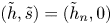 $(\tilde {h},\tilde {s}) = (\tilde {h}_n,0)$; the other two roots of
  $\tilde {h}^3 = \tilde {h}_n^3$ are complex conjugate and as such they can be left aside. The linear stability analysis around
  $(\tilde {h}_n,0)$ reveals that the fixed point is always a saddle, with two real eigenvalues of opposite sign. The physical significance of this will become clear in the course of this section.
3.2. Nullclines
A key role in the dynamics of the system is played by the nullclines given by  $f_1(\tilde {s})=0$ and
  $f_2(\tilde {h},\tilde {s})=0$, respectively. The first of these is simply the horizontal axis
  $\tilde {s}=0$. The second one has a more intricate form,
 \begin{equation} \tilde{s}_{{\pm}}(\tilde{h}) = \frac{R}{2} \left\{\tilde{h}^3 -1 \pm \sqrt{\left( \tilde{h}^3 -1 \right)^2 + \frac{4 C_f }{R } \left(1-F_n^2\tilde{h}^3 \right)}\right\}, \end{equation}
shown in figure 2(a,b) as a dashed line. Evidently, the fixed point  $(\tilde {h}_n,0)$ lies at the intersection of the two nullclines
  $\tilde {s}=0$ and
  $\tilde {s}_{\pm }(\tilde {h})$.
The latter nullcline  $\tilde {s}_{\pm }(\tilde {h})$ consists of two branches. For mild channels, these branches intersect the vertical line associated with the critical level
  $h = h_c$, i.e.
  $\tilde {h} =1$. In the case of a steep channel on the other hand, the expression under the square root in (3.2) becomes negative for
  $\tilde {h} = 1$ and its immediate neighbourhood (since
 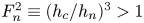 $F_n^2 \equiv (h_c/h_n)^3 > 1$ for a steep channel); as a result, the two branches of
  $\tilde {s}_{\pm }(\tilde {h})$ leave a gap around
  $\tilde {h}=1$, as seen in figure 2(b).
Inside the jump region, the nullcline  $\tilde {s}_{\pm }(\tilde {h})$ intersects the phase-space trajectories exactly at their maxima, corresponding to the inflection point of the jump (which lies close to the critical level
  $\tilde {h}=1$). Outside the jump region, on either side, the trajectories can be shown to converge to this nullcline, which thereby governs the system's asymptotic behaviour (cf. figure 2a,b). Specifically, for
  $\tilde {h} \ll 1$ the slope of
  $\tilde {h}(\tilde {x})$ is
 \begin{equation} \lim_{\tilde{h} \rightarrow 0} \tilde{s} = {\frac{R}{2}} \left( \sqrt{1+4 \frac{C_f}{R}} - 1 \right) = C_f - \frac{C_f^2 \nu }{Q} + O(\nu^2), \end{equation}
which is the correction to the classical result  $\tilde {s} \rightarrow C_f$ (in the limit for small
  $\tilde {h}$) for the slopes of the profiles
  $M3$ and
  $S3$. Note that, physically, the limit
  $\tilde {h} \rightarrow 0$ must be interpreted in such a way that
  $\tilde {h}$ always remains above a certain small but finite threshold value in order to comply with the concept of a flowing continuous medium. More specifically, in the present description all relevant lengths are supposed to remain larger than the scale at which the capillary forces would become important.
At the other end of the spectrum, for  $\tilde {h} \gg 1$, we find
  $\tilde {s} = \tan \zeta$, corresponding to a horizontal water profile with respect to the laboratory (Rouse Reference Rouse1946). As one can see in figure 2(a,b), this large-
 $\tilde {h}$ limit is already reached at
  $\tilde {h} \approx 2$. Indeed, the situation of a horizontal profile is very commonly observed in experiment, being the typical configuration encountered before a sluice gate (see figure 3).

Figure 3. Overview of the four types of hydraulic jumps that are encountered in laminar or moderately turbulent open channel flow, arising as stationary solutions of the generalized Saint-Venant equations (2.2) and (2.3). (a) The jumps  $\tilde {M}3 \rightarrow \tilde {M}1$ and
  $\tilde {M}3 \rightarrow \tilde {M}2$ (figure 2a) occur in a channel with mild slope with the aid of two sluice gates. (b) In a steep channel, the jumps
  $\tilde {S}2 \rightarrow \tilde {S}1$ and
  $\tilde {S}3 \rightarrow \tilde {S}1$ (figure 2b) are materialized in a similar manner.
3.3. Phase portraits of the hydraulic jumps
Figure 2(a) gives a detailed view of the continuous hydraulic jump in a mild channel ( $\zeta = 2^{\circ }$ and
  $F_n = 0.7$), with an effective Reynolds number
  $R=20$. For small values of
  $\tilde {h}$, where the flow is supercritical, the trajectories run close to the nullcline
  $\tilde {s}_{+}(\tilde {h})$ of (3.2). Then they depart from it, along a nearly parabolic path that follows the stable manifold of the saddle point. They cross the critical value
  $\tilde {h} =1$ close to the top of the trajectory – where the flow becomes subcritical – and descend to the close neighbourhood of the saddle
  $(\tilde {h}_n,0)$. Here the trajectories either go to the right, to the left or (in the borderline case) hit exactly upon the saddle. The red trajectory in figure 2(a) reconnects to the rightmost branch
  $\tilde {s}_{-}(\tilde {h})$ of the nullcline, forming the profile
  $\tilde {M}1$, which eventually attains the constant slope
  $\tilde {s} = \tan \zeta$. The tilde in
  $\tilde {M}1$ is used to distinguish this gradually varying profile from its non-diffusive counterpart obtained from the classic theory (Rouse Reference Rouse1946).
The blue trajectory, on the other hand, bends off to the left of the saddle, i.e. to smaller values of  $\tilde {h}$ with negative slope
  $\tilde {s}$. It decreases towards the critical level
  $\tilde {h}=1$ and can even drop below it, thereby rendering the flow supercritical again, thus permitting the flow to discharge at supercritical conditions as observed in real channels (Chow Reference Chow1973). This resolves a problematic point of the classical theory, according to which
  $M2$ (i.e. the non-diffusive counterpart of the present profile) always remained purely subcritical, meaning that the supercritical discharge, while perfectly feasible in practice, was not accounted for within the non-diffusive framework of (2.6).
However, the supercriticality of  $\tilde {M}2$ cannot be pushed too far, because at some point the height starts falling sharply towards zero (and hence the velocity
  $\bar {u}=Q/h$ diverges), meaning that our analysis breaks down. So, the blue trajectory in figure 2(a) loses its physical significance at some certain level below
  $\tilde {h}=1$. For the present study this does not matter though, since the jump (
 $\tilde {M}3 \rightarrow \tilde {M}2$) is already described by the preceding parts of the trajectory.
The jump trajectories and profiles for a steep channel are depicted in figure 2(b). The red and blue trajectories now start out from different regions of phase space, but both approach the vicinity of the saddle point  $(\tilde {h}_n,0)$, from which they escape along near-parabolic orbits that are organized around the saddle's unstable manifold. As before, they cross the critical level
  $\tilde {h}=1$ close to their maximum and when they come down again, both trajectories converge to the rightmost branch of the nullcline
  $\tilde {s}_{-}(\tilde {h})$, which represents the familiar profile with slope
  $\tilde {s} = \tan \zeta$. In analogy with the terminology from the classic non-diffusive theory, we call this the
  $\tilde {S}1$ profile.
It is apparent from the phase-space trajectories in figure 2(a,b) that the jumps for steep channels are mirror images of those for mild ones, illustrating the profound relation between these two classes of hydraulic jumps. This mirror symmetry is also reflected in the nullclines: in the mild case, the saddle point lies at the intersection of  $\tilde {s} = 0$ and the branch
  $\tilde {s}_{-}(\tilde {h})$; whereas for a steep channel the saddle lies at the intersection of
  $\tilde {s} = 0$ and
  $\tilde {s}_{+}(\tilde {h})$.
3.4. Overview of the four different jump types
The above findings are recapitulated in figure 3, presenting an overview of all four jump types in a set-up where they can be observed experimentally, involving channels with two sluice gates and an outlet (or ‘fall’). The figure is an extended and updated version of a famous textbook picture (Rouse Reference Rouse1946, p. 228). Thanks to the inclusion of a second sluice gate we can accommodate all four jump types, instead of the two types in the aforementioned picture. More importantly, owing to the diffusive term, all jump solutions are now continuous while in the classic picture they were merely vertical segments.
The symmetry between the jumps on the mild and steep channels here manifests itself as follows. The mild jump  $\tilde {M}3 \rightarrow \tilde {M}1$ is the mirror image of the steep jump
  $\tilde {S}3 \rightarrow \tilde {S}1$; to see this, one should view this latter jump upside down and trace it in reverse order, i.e. from
  $\tilde {S}1$ to
  $\tilde {S}3$. Likewise, the jump
  $\tilde {M}3 \rightarrow \tilde {M}2$ is the mirror image of
  $\tilde {S}2 \rightarrow \tilde {S}1$.
At this point, we note that the question of which jump will be realized in practice is dictated by the boundary conditions. In the case of a hydraulically mild channel, the downstream conditions decide the issue: confronted with a sluice gate,  $\tilde {M}3$ will necessarily jump to the
  $\tilde {M}1$ branch; whereas before a fall it has to follow the
  $\tilde {M}2$ branch. For a hydraulically steep channel, by contrast, the flow is controlled by the upstream conditions: any jump now has to end in
  $\tilde {S}1$, since this is the only subcritical branch, and whether it will do so from
  $\tilde {S}2$ or
  $\tilde {S}3$ depends on whether the height from which the flow starts is above or below
  $\tilde {h}_n$, respectively.
This difference between downstream and upstream control beautifully corroborates the aforementioned mirror symmetry between the jumps in mild and steep channels. The physical reason for this can be traced back to the fact that information in the supercritical regime ( $F>1$) can travel only downstream, because the fluid travels faster than any surface wave; hence the choice between
  $\tilde {S}2$ or
  $\tilde {S}3$ must necessarily be decided at the upstream end of the flow sector in question. In the subcritical regime (
 $F < 1$) information travels in both directions, which means that the choice between
  $\tilde {M}1$ and
  $\tilde {M}2$ can now be made at the downstream end of the flow sector (Rouse Reference Rouse1946). In § 5 we will come back to the propagation of information along the jump profile.
To end this section, we comment upon a central and very significant point of our dynamical systems analysis, namely the fact that the fixed point is a saddle. Keeping in mind that the fixed point  $(\tilde {h}_n,0)$ represents the uniform flow, a fully stable version of this point (a stable spiral or node) would mean that any initial condition would inevitably lead to a uniform flow. This would rule out the formation of a hydraulic jump. Conversely, a fixed point without any stable manifolds would also not do. The jump is only possible when the fixed point in question has stable as well as unstable manifolds. The stable manifold is necessary for attracting the trajectory out of the branch
  $\tilde {s}_{+}(\tilde {h})$ of supercritical flow; subsequently, the unstable manifold is needed for sending the trajectory onward to the subcritical branch
  $\tilde {s}_{-}(\tilde {h})$. It is to this delicate interplay of stability and instability that hydraulic jumps owe their existence, with the saddle
  $(\tilde {h}_n,0)$ acting as the pivotal point.
In this context, it is worth mentioning that also the existence of the hydraulic jumps found by Bohr and coworkers (Bohr et al. Reference Bohr, Putkaradze and Watanabe1997; Watanabe et al. Reference Watanabe, Putkaradze and Bohr2003) depended on the presence of a saddle point. Their dynamical system was different from ours, as mentioned below (3.1), yet the saddle point had the same function of first pulling the trajectory from the supercritical region of phase space and then pushing it on towards the subcritical region.
4. Length of the jump
4.1. Derivation of the jump length
In the jump region, the derivatives of  $\tilde {h}$ attain their maximal values and
  $d \tilde {h}/d \tilde {x}$ becomes relatively large. This implies that the term involving
  $C_f$ in (2.7) will be minor in comparison with the term linear in
  $\textrm {d} \tilde {h}/\textrm {d} \tilde {x}$, since the Chézy parameter
  $C_f$ is typically very small, of the order of 0.002–0.07, as noted under (2.3). Thus, across the jump, (2.7) is well approximated by
 \begin{equation} \tilde{h} \frac{\textrm{d}^2 \tilde{h}}{\textrm{d} \tilde{x}^2} \approx \left( \frac{\textrm{d} \tilde{h}}{\textrm{d} \tilde{x}} \right)^2 + R \left( 1 - \tilde{h}^3 \right) \frac{\textrm{d} \tilde{h}} {\textrm{d} \tilde{x}}. \end{equation}
Rewriting this second-order ODE as follows:
 \begin{equation} \tilde{h}^{{-}2} \left( \frac{\textrm{d}^2 \tilde{h}}{\textrm{d} \tilde{x}^2} \tilde{h} - \left( \frac{\textrm{d} \tilde{h}}{\textrm{d} \tilde{x}} \right)^2 \right) = R \left( \tilde{h}^{{-}2}\frac{\textrm{d} \tilde{h}}{\textrm{d} \tilde{x}} - \tilde{h} \frac{\textrm{d} \tilde{h}}{\textrm{d} \tilde{x}} \right), \end{equation}
it is readily integrated to yield
 \begin{equation} \tilde{h}^{{-}1} \frac{\textrm{d} \tilde{h}}{\textrm{d} \tilde{x} } ={-}R \left( \tilde{h}^{{-}1} + \frac{1}{2} \tilde{h}^2 \right) + B, \end{equation}
where the integration constant  $B$ is determined by the fact that the jump trajectory passes close by the saddle point
  $(\tilde {h}, \textrm {d} \tilde {h}/\textrm {d} \tilde {x}) = (\tilde {h}_n,0)$, i.e.
  $B = R (\tilde {h}_n^{-1} + {\frac {1}{2}} \tilde {h}_n^2)$
 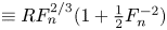 $\equiv R F_n^{2/3} (1 + {\frac {1}{2}} F_n^{-2})$. This leaves us with the following first-order ODE (cf. figure 4):
 \begin{equation} \frac{\textrm{d} \tilde{h}}{\textrm{d} \tilde{x}} ={-}\frac{1}{2} R \tilde{h}^3 + B \tilde{h} -R = A (\tilde{h}_n-\tilde{h})(\tilde{h}-\tilde{h}_1)(\tilde{h}-\tilde{h}_2), \end{equation}
where  $A = {\frac {1}{2}}R$. In the last step we have written the cubic expression in terms of its roots, by first extracting the root
  $\tilde {h}=\tilde {h}_n$ associated with the saddle point
  $(\tilde {h}_n,0)$. The other two roots
  $\tilde {h}_1, \tilde {h}_2$ are not associated with any fixed points of the full dynamical system but arise from the approximation made in (4.1). They are real-valued and of opposite sign:
  $\tilde {h}_1$ is positive (see figure 4a) and from
  $R= -A\tilde {h}_n \tilde {h}_1 \tilde {h}_2$ it may be inferred that
  $\tilde {h}_2 = -2/(\tilde {h}_n \tilde {h}_1) < 0$ (outside the scale of figure 4a).

Figure 4. (a) Phase-space trajectories for jumps on a mild chute (red and blue curves, the same as in figure 2a), together with the stable manifold (dashed curve) of the saddle point  $(\tilde {h}_n,0)$. The cubic expression (4.4), depicted by the solid black curve, is seen to be an accurate approximation to this manifold in the jump region
  $\tilde {h}_1 < \tilde {h} < \tilde {h}_n$. The vertical dashed line
  $\tilde {h} = \tilde {h}_{*}$ marks the height at which the cubic expression attains its maximum. (b) The corresponding jump profiles
  $\tilde {h}(\tilde {x})$. The solid black curve associated with the cubic approximation coincides – on the scale of this figure – with the tanh-profile equation (4.6) obtained from fitting the cubic by a parabola. The parameter values are the same as in figure 2(a).
Equation (4.4) is represented by the solid black curve in figure 4(a) and is seen to give a very good approximation of the saddle's manifold (dashed black curve) in the jump region. Its maximum lies at  $\tilde {h} = \tilde {h}_{*} = (2B/3R)^{1/2} = [ {\frac {2}{3}} (\tilde {h}_n^{-1} + {\frac {1}{2}} \tilde {h}_n^2 ) ]^{1/2}$, indicated by the vertical dashed line in figure 4(a). With an eye to the analysis to follow, we note that the depicted lobe of the cubic function can be fitted closely to a parabola.
Equation (4.4) is a separable ODE. It may be cast in the form  $\textrm {d}\tilde {x}=\textrm {d}\tilde {h}/[A (\tilde {h}_n-\tilde {h})(\tilde {h}-\tilde {h}_1)(\tilde {h}-\tilde {h}_2)]$ and then be solved analytically by decomposing the right-hand side into its partial fractions. The result is an elaborate expression involving logarithms. For our purposes, however, it is sufficient to focus upon the jump region, where the cubic expression can be replaced – without any significant loss of accuracy – by a parabola of the form
  $\tilde {s}(\tilde {h})= \tilde {s}_{*} - K(\tilde {h}-\tilde {h}_{*})^2$, with
  $K=\tilde {s}_{*}/(\tilde {h}_n-\tilde {h}_{*})^2$. This parabolic approximation is symmetric around
  $\tilde {h}_{*}$ and its apex
  $\tilde {s}_{*} = \tilde {s}(\tilde {h}_{*}) \equiv \textrm {d} \tilde {h}/\textrm {d} \tilde {x} \vert _{\tilde {h}=\tilde {h}_{*}}$ coincides with the local maximum of the cubic expression (4.4). The parabola intersects the horizontal axis at the points
  $(\tilde {h}_n,0)$ and
  $(2\tilde {h}_{*}-\tilde {h}_n,0)$.
Thus, in the jump region equation (4.4) is well approximated by
 \begin{equation} \frac{\textrm{d} \tilde{h}}{\textrm{d} \tilde{x}} = \frac{\tilde{s}_{*}}{\left(\tilde{h}_n - \tilde{h}_{*} \right)^2} \left(\tilde{h}_n -\tilde{h}\right) \left(\tilde{h} -(2\tilde{h}_{*} - \tilde{h}_n)\right), \end{equation}
which can be integrated to yield
 \begin{equation} \tilde{h}(\tilde{x}) \approx \tilde{h}_{*} + (\tilde{h}_n-\tilde{h}_{*}) \tanh \left( \alpha \tilde{x} \right),\quad \textrm{where}\ \alpha = \frac{\tilde{s}_{*}}{\tilde{h}_n-\tilde{h}_{*}}. \end{equation}
The integration constant here has been chosen such that the jump is centred around  $\tilde {x}=0$, i.e.
  $\tilde {h}(0)= \tilde {h}_{*}$. The approximate profile equation (4.6) traverses the jump amplitude
  $2(\tilde {h}_n-\tilde {h}_{*})$ in a symmetrical fashion. The jump region of figure 4(a,b) shows that this is an adequate description, and that especially in the upper half of the jump it is excellent. (For steep jumps this would be the lower half, as can be seen in the insets of figure 5.)

Figure 5. (a) The non-dimensional length  $\tilde {L}$ predicted by (4.7) as a function of
  $F_n$ (the Froude number at the reference level
  $\tilde {h}=\tilde {h}_n$), for a fixed value of the effective Reynolds number
  $R=20$. The regime of hydraulically mild (M) channels corresponds to
  $0 < F_n < 1$ and that of steep (S) channels to
  $F_n > 1$. The intermediate grey zone around
  $F_n=1$ indicates that the prediction (4.7) becomes unreliable here. The insets are representative jumps for the mild and steep cases. The dashed curves depict the actual profiles, corresponding to the stable/unstable manifold of the saddle point
  $(\tilde {h}_n,0)$, whereas the solid black curves are the approximative tanh-profiles given by (4.6). (b) Phase-space portrait for a hydraulically critical channel (
 $F_n=1$). The trajectories are seen to be completely symmetric around
  $\tilde {h}_n =\tilde {h}_c = 1$, in accordance with the fact that (being on the borderline between mild and steep) they have to be their own mirror image. The manifolds of the saddle point connect directly – without detours – to the nullclines at either side, so there is no backbone here for a near-parabolic orbit. As a result, in this case the transition from supercritical to subcritical flow takes place without any pronounced jump; note the small scale of the
  $\tilde {s}$-axis.
Now, the non-dimensional jump length  $\tilde {L}$ may be defined as the distance in the
  $\tilde {x}$-direction in which
  $\tilde {h}(\tilde {x})$ completes
  $99\,\%$ of its course from
  $\tilde {h}_1$ to
  $\tilde {h}_n$. Since
  $\tanh (\alpha \tilde {x}) = 0.99$ at
  $\alpha \tilde {x} = 2.65$, this gives
  $\tilde {L} = 2 \times 2.65/ \alpha = 5.3 (\tilde {h}_n-\tilde {h}_{*})/ \tilde {s}_{*}$. With
  $\tilde {s}_{*} \equiv \textrm {d} \tilde {h}/\textrm {d} \tilde {x} (\tilde {h}_{*})$ from (4.4), and expressing all relevant heights in terms of
  $F_n$ and
  $R$, we arrive at
 \begin{equation} \tilde{L} = 5.3\frac{6 F_n^{4/3}}{R \left \vert 1-4F_n^2+\sqrt{3+6 F_n^2}\right \vert}. \end{equation}
For the jumps shown in figure 2(a) (and figure 4) with  $F_n=0.7$ and
  $R=20$, the above expression predicts a length
  $\tilde {L} = 0.69$. This is in excellent agreement with the value obtained from numerically solving the full dynamical system (3.1a) and (3.1b).
The same expression (4.7) holds for jumps on a steep channel. In this case, the fixed point  $(\tilde {h}_n,0)$ lies at the left-hand side of the jump region (i.e. the supercritical side) and the associated value of
  $F_n$ is larger than
  $1$. To keep
  $\tilde {L}$ positive, the absolute value signs in the denominator are then needed. For the jump depicted in figure 2(b), with
  $F_n=1.4$ and
  $R=20$, (4.7) yields
  $\tilde {L} = 0.83$, once again in full agreement with the length found from solving the full dynamical system.
4.2. Discussion of the expression for the jump length
In figure 5(a), the length  $\tilde {L}$ predicted by (4.7) is plotted as a function of
  $F_n$, for a fixed value of the effective Reynolds number (
 $R=20$). The left-hand part of the diagram regime (
 $0 < F_n < 1$) corresponds to hydraulically mild channels and is denoted by the letter M. As the inset shows, in this case the reference point – where
  $F_n$ is measured – lies at the upper, subcritical side of the jump. The right-hand part (
 $F_n > 1$) corresponds to the steep regime denoted by the letter S. Here, in accordance with the mirror symmetry discussed in the previous section, the reference point is located at the lower, supercritical side of the jump. Also the form of the plot of
  $\tilde {L}(F_n)$ itself, with its two hyperbolic-like branches around
  $F_n=1$, is again a consequence of the mirror symmetry between jumps on mild and steep channels.
Between the mild and steep regimes lies the critical value  $F_n =1$, for which the expression (4.7) diverges and the length prediction breaks down. The grey zone shrouding
  $F_n =1$ signifies the region in which (4.7) does not accurately represent the jump length anymore. The reason for this breakdown lies in the fact that the approximation on which (4.7) was based, namely that
  $\textrm {d} \tilde {h}/\textrm {d} \tilde {x}$ becomes sufficiently large compared with
  $C_f$, loses its validity as one comes too close to the critical channel conditions. In figure 5(b) we show the phase portrait for the exact value
  $F_n=1$ (and
  $R=20$): the stable and unstable manifolds emanating from the saddle do not make any near-parabolic detour here, but connect directly to the nullclines. Hence, also the trajectories that represent the transition from supercritical to subcritical flow (red solid curves) do not need to become large. This means that the last term in (2.7) cannot be neglected in the critical case, and hence one should not use the approximative equation (4.1), which formed the basis of the analysis leading to the length prediction (4.7). Physically, on a critically sloped channel, the transition from the supercritical to the subcritical flow profiles can take place either via a slight jump (upper red curve) or via an extended flow segment where the slope is actually smaller than in the surrounding gradually varied profiles (lower red curve). Also a transition without any discernible change of slope is possible in this case; this would correspond to a linearly thickening fluid profile aligned with the horizon,
  $\tilde {h}(\tilde {x}) = \tilde {x} \tan \zeta$. One should note, however, that it will require a high degree of fine-tuning to produce such critical channel conditions in experiments.
Outside the grey zone, where (4.7) is valid, this expression reflects that the jumps considered here result from an interplay between gravity and viscous diffusion, represented by the Froude number  $F_n$ and the effective Reynolds number
  $R$, respectively. With respect to the latter, we observe that
  $\tilde {L}$ is inversely proportional to
  $R$, i.e. it grows linearly with
  $\nu$, which stands to reason given the flattening effect of the diffusion. In the non-diffusive limit
  $\nu \rightarrow 0$ (or equivalently,
  $R \rightarrow \infty$) the length vanishes, reproducing the infinitely steep jump of the classical analysis.
The more intricate dependence on the Froude number  $F_n$ is illustrated in figure 5(a). Since the present study – based on the generalized Saint-Venant equations – concerns weak jumps as are found in laminar and moderately turbulent flow, the Froude number of the incoming flow should not exceed
  $2.5$. This immediately puts an upper bound on the admissible values of
  $F_n$ in the steep regime, for which the reference point (
 $\tilde {h}_n$) is positioned at the supercritical side of the jump. Likewise, in the mild regime,
  $F_n$ should not become too small, since the limit
  $F_n \rightarrow 0$ corresponds to a situation in which the upper flank of the jump connects to a flow that is very thick and extremely slow. This limit must be treated with caution, since such a thick flow is beyond the scope of the generalized Saint-Venant equations (2.2) and (2.3), which are meant to describe shallow fluid flow.
5. Stability of the jumps
5.1. Numerical experiment
The previous sections have provided insight into the structure of the jumps from a dynamical systems point of view. This method has given us a geometric overview of the stationary solutions of the generalized Saint-Venant equations, yet it does not reveal the time-dependent dynamics leading up to these solutions, nor does it give information about their stability against perturbations. To shed light upon this issue, we must return to the original PDEs (2.2) and (2.3).
In this section we will be concerned in particular with the stability question and we will show that the jump profiles obtained via the dynamical systems approach are stable against small perturbations. In this context, we pay special attention to the direction in which these perturbations propagate along the profile. We will see that a perturbation on the supercritical lower branch ( $F>1$) can make itself be felt only in the downstream direction, whereas a perturbation on the subcritical upper branch (where
  $F<1$) sends small waves in both directions. In fact, the one-way propagation of information in the supercritical regime has given rise to an intriguing analogy between hydraulic jumps and white holes in cosmology (Volovik Reference Volovik2005; Jannes et al. Reference Jannes, Piquet, Maïssa, Mathis and Rousseaux2011).
For the numerical integration we use the ‘method of lines’ (Schiesser Reference Schiesser1991; Hamdi, Schiesser & Griffiths Reference Hamdi, Schiesser and Griffiths2007). This method transforms the two PDEs (2.2) and (2.3) into a system of multiple ODEs, by discretizing the spatial variable  $x$ (to a uniform grid
  $x_0 \leq x_i \leq x_{{max}}$ in steps of
  ${\rm \Delta} x$, and using a central-difference scheme to approximate the spatial derivatives), leaving
  $t$ as the only continuous independent variable. Our standard grid spacing is
  ${\rm \Delta} x = 0.001$, which means, for example, for the simulation of figure 6 (which concerns
  $4$ metres along the
  $x$-axis) that the interval is divided in
  $4000$ steps. The resulting system of ODEs then consists of
  $4001$ equations per PDE, leading to a total of
  $8002$ coupled ODEs. The accuracy of the results has been checked by repeating the procedure for smaller values of the grid spacing as well.

Figure 6. Stability of the hydraulic jump  $\tilde {S}3 \rightarrow \tilde {S}1$. Perturbations
  ${A}_0$ and
  ${B}_0$ (indicated by the black dashed humps) are imposed on the jump's lower and upper branch, and their subsequent evolution is computed from the generalized Saint-Venant equations (2.2) and (2.3). Both perturbations are seen to break into two wave packets that decay with time, evidencing the stability of the jump. (a) Supercritical branch: the two wave packets,
  ${A}^{+}(t)$ and
  ${A}^{-}(t)$, are depicted at the consecutive moments
  $t_1 = 0.2$ s (red),
  $t_2=0.4$ s (green) and
  $t_3=0.6$ s (blue). Both packets propagate downstream and eventually pass the critical level
  $h=h_c$, where they enter the subcritical regime; at
  $t=t_3$ the wave packet
  ${A}^{+}(t)$ has just made this transition. (b) Subcritical branch: the wave packets
  ${B}^{+}(t)$ and
  ${B}^{-}(t)$ are again depicted at times
  $t_1$,
  $t_2$ and
  $t_3$. They are seen to travel in both directions. At
  $t=t_3$ the one going downstream,
  ${B}^{+}(t)$, has already advanced beyond the plot frame. The packet moving upstream,
  ${B}^{-}(t)$, can never cross
  $h = h_c$, so it gets trapped (and dies out) on the upper flank of the jump.
The initial conditions used in figure 6 are the perturbed jump profile  $h(x,0)$ (dashed black line) and the corresponding initial velocity
  $\bar {u}(x,0) = Q/h(x,0)$, taken at the grid points
  $x=x_i$,
  $i=0,\ldots ,4000$. As for the required boundary conditions (one for
  $h$ and two for
  $\bar {u}$, since the generalized Saint-Venant equations contain only first-order spatial derivatives of
  $h$ and up to second-order spatial derivatives of
  $\bar {u}$): at the upstream boundary
  $x_0$ we impose Dirichlet conditions for
  $h$ and
  $\bar {u}$; whereas at the downstream end
  $x_{{max}}$ we employ a Neumann condition for
  $\bar {u}$.
In figure 6(a,b) we show snapshots from a numerical experiment in which we follow the time evolution of a perturbation on the supercritical and subcritical branch, respectively, of a jump  $\tilde {S}3 \rightarrow \tilde {S}1$ on a steep channel. The initial perturbation (dashed black curve) is a Gaussian-shaped hump superimposed on the profile obtained from the dynamical system. This perturbation sends out wave packets that are seen to decay with time, confirming the stability of the jump.
5.2. Linear stability analysis: propagation and attenuation of small perturbations
Another thing that is confirmed by the numerical experiment is the aforementioned difference in propagation of the wave packets, which is indeed unidirectional on the supercritical branch and bidirectional on the subcritical one. This phenomenon can be understood from the governing generalized Saint-Venant equations, (2.2) and (2.3), by linearizing them around a base flow with constant height  $h_0$ and associated depth-averaged velocity
  $u_0$.
That is, we set  $h(x,t) = h_0 + \hat {h}(x,t)$ and
  $\bar {u}(x,t) = u_0+\hat {u}(x,t)$ and keep only the linear terms with respect to the perturbations
  $\hat {h}(x,t)$ and
  $\hat {u}(x,t)$. The linearized continuity equation and momentum balance then take the form
 \begin{gather} \hat{h}_t + u_0 \hat{h}_x + h_0 \hat{u}_x = 0, \end{gather}
 \begin{gather}\hat{u}_t + u_0 \hat{u}_{x} = g\sin \zeta - g\cos \zeta \hat{h}_x - C_f \frac{u_0^2}{h_0} \left(1-\frac{\hat{h}}{h_0} + 2 \frac{\hat{u}}{u_0}\right)+ \nu \hat{u}_{xx}, \end{gather}
where the friction term featuring in (5.1b) comes about as follows:
 \begin{equation} C_f \frac{(u_0+\hat{u})^2}{h_0+\hat{h}}=\frac{C_f u_0^2}{h_0} \frac{\left(1+\hat{u}/u_0\right)^2}{1+\hat{h}/h_0} \approx \frac{C_f u_0^2}{h_0}\left(1+2\frac{\hat{u}}{u_0}\right)\left(1-\frac{\hat{h}}{h_0}\right). \end{equation}
Rearranging the linearized continuity equation (5.1a), one has
 \begin{equation} \hat{u}_x ={-}\frac{1}{h_0} \left(\hat{h}_t + u_0\hat{h}_x \right), \end{equation}
and from this, by successive differentiations, one finds  $\hat {u}_{xx}$,
  $\hat {u}_{xxx}$ and
  $\hat {u}_{xt}$. These in turn can be substituted into the linearized momentum balance (5.1b) after this has been differentiated with respect to
  $x$, to arrive at an equation in terms of
  $\hat {h}$ only. The resulting equation reads
 \begin{equation} \hat{h}_{tt} +2 u_0 \hat{h}_{xt}+ u_0^2 \hat{h}_{xx} = g h_0 \cos \zeta \hat{h}_{xx}-3 \frac{C_f u_0^2}{h_0} \hat{h}_{x}-2 \frac{C_f u_0}{h_0}\hat{h}_{t}+ \nu \hat{h}_{xxt}+\nu u_0 \hat{h}_{xxx}, \end{equation}
which can be cast in non-dimensional form by introducing  $\hat {h}=h_0\tilde {h}$,
  $x=h_0\tilde {x}$ and
  $t=(h_0/u_0)\tilde {t}$ as follows:
 \begin{equation} \tilde{h}_{\tilde{t}\tilde{t}}+ 2 \tilde{h}_{\tilde{x}\tilde{t}} + \left(1-\frac{1}{F^2} \right)\tilde{h}_{\tilde{x}\tilde{x}} + 3 C_f \tilde{h}_{\tilde{x}} + 2 C_f \tilde{h}_{\tilde{t}} - \frac{1}{R} \left(\tilde{h}_{\tilde{x}\tilde{x}\tilde{t}}+\tilde{h}_{\tilde{x}\tilde{x}\tilde{x}} \right) =0. \end{equation}
 By inserting the travelling wave ansatz  $\tilde {h}(\tilde {x},\tilde {t}) = A \exp ({\textrm {i}(\tilde {k}\tilde {x}-\tilde {\omega } \tilde {t})})$ into (5.5), with
  $\tilde {k}$ and
  $\tilde {\omega }$ being the dimensionless wavenumber and angular frequency, respectively, we obtain the dispersion equation
 \begin{equation} \tilde{\omega}^2 - 2 \left(\tilde{k} - \textrm{i} \left(C_f+ \frac{\tilde{k}^2}{2R} \right) \right) \tilde{\omega} + \left( \left(1-\frac{1}{F^2}\right)\tilde{k}^2 - \textrm{i} \left( 3 C_f \tilde{k} + \frac{\tilde{k}^3}{R} \right) \right)=0, \end{equation}
which is a quadratic equation for  $\tilde {\omega }$. It has the following two solutions:
 \begin{equation} \tilde{\omega}_{{\pm}}(\tilde{k}) = \tilde{k} -\textrm{i}\left( C_f + \frac{\tilde{k}^2}{2R} \right) \pm \sqrt{-C_f^2 + \left(\frac{1}{F^2}-\frac{C_f}{R} \right) \tilde{k}^2 - \frac{\tilde{k}^4}{4R^2} + \textrm{i} C_f \tilde{k}}. \end{equation}
The real and imaginary parts of (5.7) are
 \begin{equation} \textrm{Re}[\tilde{\omega}_{{\pm}}(\tilde{k})] = \tilde{k} \pm M^{{1}/{2}}(\tilde{k}) \cos \left( \frac{\phi(\tilde{k})}{2} \right) \end{equation}
and
 \begin{equation} \textrm{Im}[\tilde{\omega}_{{\pm}}(\tilde{k})] ={-}C_f - \frac{\tilde{k}^2}{2R} \pm M^{{1}/{2}}(\tilde{k}) \sin \left( \frac{\phi(\tilde{k})}{2} \right), \end{equation}
respectively, where  $M(\tilde {k})$ denotes the magnitude of the (complex) quantity under the square root of (5.7),
 \begin{equation} M(\tilde{k}) = \left[ \left({-}C_f^2 + \left( \frac{1}{F^2} -\frac{C_f}{R} \right) \tilde{k}^2 -\frac{\tilde{k}^4}{4R^2} \right)^2 + \left( C_f \tilde{k} \right)^2 \right]^{1/2} \end{equation}
and  $\phi (\tilde {k})$ is its principal argument,
 \begin{equation} \phi(\tilde{k}) = \textrm{Arg} \left({-}C_f^2 + \left( \frac{1}{F^2} -\frac{C_f}{R} \right) \tilde{k}^2 -\frac{\tilde{k}^4}{4R^2} + \textrm{i} C_f\tilde{k}\right). \end{equation}
 In figure 7 we show the real and imaginary parts of  $\tilde {\omega }_{\pm }(\tilde {k})$ for typical values of the parameters
  $R$,
$R$,  $C_f$ and
  $F$. The effective Reynolds number and the dimensionless friction factor are
  $R=20$ and
  $C_f=0.02$, just as in figure 6, while for the Froude number we have chosen the values
  $F=1.57$ for
  $\tilde {\omega }_{+}(\tilde {k})$ (panel (a)) and
  $F=1.70$ for
  $\tilde {\omega }_{-}(\tilde {k})$ (panel (b)) associated with the green wave packets at
  $t=t_2$ on the supercritical branch of figure 6(a).

Figure 7. The real and imaginary parts of  $\tilde {\omega }_{\pm }(\tilde {k})$, given by (5.8) and (5.9), represented by the red and blue curves, respectively. Also depicted (as a black dashed line) is the approximate expression
  $(1 \pm 1/F) \tilde {k}$ for the real part
  $\textrm {Re}[\tilde {\omega }_{\pm }(\tilde {k})]$. This approximation is seen to be very accurate for small
  $\tilde {k}$, and therefore relevant for our analysis, since the wave packets are localized entities composed of harmonic waves with small wavenumbers
  $\tilde {k}$. Their phase speed
  $\textrm {Re}[\tilde {\omega }_{\pm }(\tilde {k})] / \tilde {k}$ is thus in good approximation given by
  $1 \pm 1/F$. The negative value of the imaginary part
  $\textrm {Im}[\tilde {\omega }_{\pm }(\tilde {k})]$ is responsible for the observed decay of the wave packets with time. Parameter values:
  $R=20$,
  $C_f=0.02$,
  $F=1.57$ for
  $\tilde {\omega }_{+}(\tilde {k})$ (a) and
  $F=1.70$ for
  $\tilde {\omega }_{-}(\tilde {k})$ (b), corresponding to the green wave packets at
  $t=t_2$ on the supercritical branch of figure 6(a).
The fact that  $\tilde {\omega }(\tilde {k})$ is complex, with a real and imaginary part, means that the plane wave components comprising the wave packet have the following form:
 \begin{equation} \tilde{h}(\tilde{x},\tilde{t}) = A \exp({{\textrm{Im}}[\tilde{\omega}(\tilde{k})]\tilde{t}}) \exp({\textrm{i}(\tilde{k}\tilde{x}- {\textrm{Re}}[\tilde{\omega}(\tilde{k})]\tilde{t})}). \end{equation}
The first exponential on the right-hand side of (5.12) shows that the amplitude of the wave packet increases or decreases exponentially with time, as  $\exp ({{\textrm {Im}}[\tilde {\omega }(\tilde {k})]\tilde {t}})$. In our system, as figure 7 shows, the imaginary part
  $\textrm {Im}[\tilde {\omega }(\tilde {k})]$ is always negative and hence the amplitude diminishes. More specifically, the wave packets shown in figure 6 are composed of harmonic waves with an average dimensionless wavenumber
  $\tilde {k}^{*} = 0.7 \pm 0.1$ and the corresponding values
  $\textrm {Im}[\tilde {\omega }_{+}(\tilde {k}^{*})] = -0.016$ and
  $\textrm {Im}[\tilde {\omega }_{-}(\tilde {k}^{*})] = -0.015$ are in full agreement with the observed exponential attenuation of the waves.
The second exponential in (5.12) determines the (dimensionless) phase speed  $\tilde {c}_{\pm }(\tilde {k})$ of the harmonic waves in question, which is given by
 \begin{equation} \tilde{c}_{{\pm}}(\tilde{k}) = \frac{\textrm{Re}[\tilde{\omega}_{{\pm}}(\tilde{k})]}{\tilde{k}}. \end{equation}
In the inviscid limit for  $C_f \rightarrow 0$ (no shear stresses) and
  $1/R \rightarrow 0$ (no in-plane stresses) (5.7) reduces to
  $\tilde {\omega }_{\pm }(\tilde {k}) = (1 \pm F^{-1})\tilde {k}$. So the angular frequency
  $\tilde {\omega }_{\pm }(\tilde {k})$ in the inviscid case is purely real, implying that the waves are not attenuated; this makes sense, since the absence of viscosity deprives the system of its source of dissipation. The phase speed (5.13) in this limit becomes independent of the wavenumber
  $\tilde {k}$ as follows:
 \begin{equation} \tilde{c}_{{\pm},{{inv}}}(F) = 1 \pm \frac{1}{F}. \end{equation}
Moreover, in this inviscid limit also the group velocity  $\tilde {c}_{g} = \textrm {d} \tilde {\omega } / \textrm {d}\tilde {k}$ becomes identical to the same expression (5.14), so the absence of the viscous terms also means that the system is rendered dispersionless. The small-amplitude wave packets then behave as non-dispersive waves.
As a matter of fact, the propagation speed given by (5.14) also provides a good approximation for the actual situation under consideration. Not only are the parameters  $C_f$ and
  $1/R$ quite small in our system, but importantly, the wavenumbers
  $\tilde {k}$ are small as well. Indeed, as figure 7 shows,
  $\textrm {Re}[\tilde {\omega }_{\pm }(\tilde {k})]$ and
  $(1 \pm F^{-1})\tilde {k}$ are practically identical in the range
  $\tilde {k} \lesssim 1$ we are dealing with. We thus arrive at the conclusion that the small-amplitude perturbations (which lend themselves to the present linearized description) behave as attenuated, yet nearly non-dispersive waves propagating at speeds
  $\tilde {c}_{\pm }(F)=(1 \pm F^{-1})$ depending solely on the Froude number
  $F = \bar {u}_0/\sqrt {gh_0 \cos \zeta }$ of the base flow.
When the base flow is supercritical ( $F>1$), both velocities
  $\tilde {c}_{\pm }(F)$ are positive; so all perturbations travel in the upstream direction. On the other hand, in the subcritical regime with
  $F<1$ the velocity
  $\tilde {c}_{-}(F)$ becomes negative, corresponding to upstream propagation, whereas
  $\tilde {c}_{+}(F)$ remains positive. This explains the unidirectional and bidirectional propagation observed in figures 6(a) and 6(b), respectively.
On the supercritical branch of figure 6(a) we measure the (dimensional) velocities  $c_{-} \approx 0.73$ and
  $c_{+} \approx 2.80\ \textrm {m}\ \textrm {s}^{-1}$, corresponding to the dimensionless values
  $\tilde {c}_{-} = c_{-}/u_0 \approx 0.41$ and
  $\tilde {c}_{+} = c_{+}/u_0 \approx 1.65$. In agreement with this, the theoretical approximation equation (5.14) gives the propagation speeds
  $\tilde {c}_{-} = 0.41$ and
  $\tilde {c}_{+} = 1.64$, respectively.
Likewise, on the subcritical branch of figure 6(b) we find from our numerical simulations  $c_{-} \approx -0.60$ and
  $c_{+} \approx 2.40\ \textrm {m}\ \textrm {s}^{-1}$, corresponding to the dimensionless values
  $\tilde {c}_{-} \approx -0.67$ and
  $\tilde {c}_{+} \approx 3.28$. Equation (5.14) in this case predicts
  $\tilde {c}_{-} = -0.66$ and
  $\tilde {c}_{+} = 3.25$, once again in accordance with the numerically observed values. Given the approximation we have made by truncating the mass and momentum balance at the linear order in
  $\hat {h}$ and
  $\hat {u}$, and given that the base flow along the jump is actually not precisely uniform (as assumed in the above analysis), the agreement may be said to be very satisfactory.
6. Conclusion
The hydraulic jumps in laminar or moderately turbulent open channel flow have been captured, complete with their mean-field shock structure, as stationary solutions of the generalized Saint-Venant equations. In phase space, the jumps manifest themselves as trajectories that leap from the supercritical branch of the nullcline to the opposite subcritical branch via a pronounced near-parabolic orbit. This orbit follows the stable/unstable manifold of the saddle point  $(\tilde {h},\tilde {h}') = (\tilde {h}_n,0)$, for mild/steep channels, respectively, while the nullcline
  $\tilde {s}_{\pm }(\tilde {h})$ given by (3.2) provides the form of the gradually varied profiles before and after the jump.
The phase-space representation has yielded a very useful geometrical insight into the structure of the jumps. Among other things, it has brought to light the mirror symmetry that exists between the jumps in mild and steep channels. This is illustrated by figure 2 and also the overview in figure 3, where the two jump types that can be found in mild channels are presented along with their two counterparts for steep channels.
The dynamical systems description has also led to the derivation of the approximative expression (4.7) for one of the most prominent features of the hydraulic jump, namely, its length. To the best of our knowledge, this is the first analytic expression for the length extracted directly from the governing equations. It will be very interesting to test the accuracy of this prediction in experiment.
Finally, the important issue of the stability of the jumps has been settled by returning to the original PDEs. The jump profiles obtained from the dynamical systems analysis are inserted into (2.2) and (2.3), with perturbations applied to the supercritical and subcritical branches, respectively. The perturbations are seen to decay with time, as illustrated in figure 6 and corroborated by means of a linear stability analysis. Thus the stability of the jumps is confirmed.
Acknowledgements
The authors would like to thank Professors G.M. Horsch, J. Tsamopoulos (University of Patras, Greece), T.E. Karakasidis and A. Liakopoulos (University of Thessaly, Greece) for stimulating remarks and their keen interest in this work.
Declaration of interests
The authors report no conflict of interest.


 Open access