


1. Introduction
The occurrence of temperature differences and the resulting buoyancy forces induce complex fluid motions in many geophysical and astrophysical settings and technical systems (Kadanoff Reference Kadanoff2001; Verma Reference Verma2018). This is one reason why thermally driven fluid flows have been investigated comprehensively in the past decades in theory, simulation and laboratory experiments. Of central interest is a better understanding of the close link between structure formation and the resulting turbulent heat transport properties. In this context, the Rayleigh–Bénard model has been established as one of the most frequently considered basic configurations (Bodenschatz, Pesch & Ahlers Reference Bodenschatz, Pesch and Ahlers2000; Ahlers, Grossmann & Lohse Reference Ahlers, Grossmann and Lohse2009; Chillà & Schumacher Reference Chillà and Schumacher2012). This simple convection model consists of a fluid layer between two parallel plates, which is heated uniformly from below and cooled from above, enclosed by adiabatic side walls. If the driving due to the vertical temperature gradient is large enough, then turbulent Rayleigh–Bénard convection (RBC) develops in the layer that carries heat from the bottom to the top. Even though the model cannot represent the full complexity of most natural and technical systems (see e.g. Schumacher & Sreenivasan (Reference Schumacher and Sreenivasan2020) for the case of convection in the solar interior), it turned out to be very useful for studies of fundamental turbulence characteristics in thermal convection, which also motivates our present study.
In this work, turbulent superstructures of convection – a gradually evolving large-scale order in horizontally extended layers with a coherence length larger than the layer height – are investigated in controlled laboratory experiments. The characteristic scale and dynamical evolution of superstructures is studied by a combination of stereoscopic particle image velocimetry (PIV) and thermometry enabling a joint experimental determination of the local structure of the three velocity components  $u_x$,
  $u_y$ and
  $u_z$, and the temperature
  $T$, as fields in a larger horizontal cross-sectional plane. This opens the way to an experimental investigation of the spatial structure of the local convective heat flux, its fluctuations, and thus also the global heat transfer across the layer. Our long-term experiments are conducted in water at Prandtl number
  $Pr=7$ in a cell with a square cross-section and aspect ratio
  $\varGamma =l/h=25$, with
  $l$ being the horizontal length and
  $h$ the height of the fluid layer. Furthermore, we compare the experimental results with existing direct numerical simulation (DNS) data for the same parameter range, which will be detailed later. Characteristic length scales and times are found to be in the same range as the numerical results. We also compare the statistics of the local convective heat flux, the velocity and temperature fields, and discuss differences that can be traced back to resolution effects in the experiments.
The ‘large-scale order’ in the form of superstructures in fully developed, horizontally extended convective turbulence has been analysed with regard to the characteristic length scales for different Rayleigh and Prandtl numbers (Hartlep, Tilgner & Busse Reference Hartlep, Tilgner and Busse2003; Parodi et al. Reference Parodi, von Hardenberg, Passoni, Provenzale and Spiegel2004; Pandey, Scheel & Schumacher Reference Pandey, Scheel and Schumacher2018; Lenzi, von Hardenberg & Provenzale Reference Lenzi, von Hardenberg and Provenzale2021; Pandey, Schumacher & Sreenivasan Reference Pandey, Schumacher and Sreenivasan2021), the associated dependence of the turbulent heat transfer on the aspect ratio of the convection layer (Bailon-Cuba, Emran & Schumacher Reference Bailon-Cuba, Emran and Schumacher2010), and the effect of the aspect ratio on the characteristic pattern scale (von Hardenberg et al. Reference von Hardenberg, Parodi, Passoni, Provenzale and Spiegel2008; Stevens et al. Reference Stevens, Blass, Zhu, Verzicco and Lohse2018). In the studies of Emran & Schumacher (Reference Emran and Schumacher2015) and Sakievich, Peet & Adrian (Reference Sakievich, Peet and Adrian2016), it has been demonstrated that the large-scale structures rearrange slowly over time. The characteristic length and time scales of the superstructures, as determined by Pandey et al. (Reference Pandey, Scheel and Schumacher2018) on the basis of numerical simulations in the Eulerian frame of reference, have also been confirmed in a complementary analysis of Lagrangian trajectory clusters (Schneide et al. Reference Schneide, Pandey, Padberg-Gehle and Schumacher2018; Vieweg et al. Reference Vieweg, Schneide, Padberg-Gehle and Schumacher2021b). Deep learning algorithms have been applied to parametrize the turbulent convective heat flux in global models by a reduction to a planar dynamical network assessing the amount of heat transported by superstructures in Fonda et al. (Reference Fonda, Pandey, Schumacher and Sreenivasan2019). Moreover, the coherence of the superstructures in the temperature and velocity field has been investigated recently in detail by Krug, Lohse & Stevens (Reference Krug, Lohse and Stevens2020) and Blass et al. (Reference Blass, Verzicco, Lohse, Stevens and Krug2021), while the interplay between small-scale turbulent fluctuations and the large-scale turbulent superstructures has been studied by Green et al. (Reference Green, Vlaykov, Mellado and Wilczek2020), Berghout, Baars & Krug (Reference Berghout, Baars and Krug2021), and Valori & Schumacher (Reference Valori and Schumacher2021).
All studies of turbulent superstructures cited above are based on DNS of the Boussinesq equations. The number of experimental investigations of turbulent convection in large-aspect-ratio cells with  $\varGamma \gg 1$ is much smaller. Fitzjarrald (Reference Fitzjarrald1976) measured co-spectra of the temperature and velocity in air at Prandtl number
  $Pr = 0.7$ with local sensor elements, and determined a Rayleigh number dependence of the characteristic convection pattern scale. The large-scale structures in RBC have also been visualized in experiments with different working fluids at higher Prandtl numbers and moderate Rayleigh numbers via the shadowgraph technique (Busse & Whitehead Reference Busse and Whitehead1971, Reference Busse and Whitehead1974; Busse Reference Busse1994) or photography (Krishnamurti & Howard Reference Krishnamurti and Howard1981). Fluctuation profiles of the velocity and temperature across the layer were investigated by Adrian (Reference Adrian1996). Turbulent superstructure patterns have been obtained in convection experiments in air by Kästner et al. (Reference Kästner, Resagk, Westphalen, Junghähnel, Cierpka and Schumacher2018) and Cierpka et al. (Reference Cierpka, Kästner, Resagk and Schumacher2019) by time-averaged velocity fields that were measured with PIV (Raffel et al. Reference Raffel, Willert, Scarano, Kähler, Wereley and Kompenhans2018).
Our experiment has been set up to perform simultaneous measurements of the temperature and velocity fields over long time intervals in a large section of the horizontal mid-plane of a Rayleigh–Bénard cell. We therefore suspend thermochromic liquid crystals (TLCs) in the flow that change their colour with respect to the local temperature (Dabiri Reference Dabiri2008; Moller, Resagk & Cierpka Reference Moller, Resagk and Cierpka2021). TLCs have also been used in RBC experiments by Zhou, Sun & Xia (Reference Zhou, Sun and Xia2007) to analyse the morphology of thermal plumes in a cylindrical cell with  $\varGamma =1$. However, these particles serve in the current case not only as temperature sensors, but also as tracer particles for stereoscopic PIV measurements, and thus enable the simultaneous velocity and temperature measurements (see also Schmeling, Bosbach & Wagner (Reference Schmeling, Bosbach and Wagner2014)). On the basis of these measurements, the strong influence of the turbulent superstructures on the local convective heat flux is demonstrated. In addition, their horizontal extent, as well as their reorganization over longer time intervals, is analysed. In order to assess both the experimental and numerical investigations of turbulent superstructures in RBC, the results of the measurements are compared with those of DNS performed previously by Pandey et al. (Reference Pandey, Scheel and Schumacher2018) and Fonda et al. (Reference Fonda, Pandey, Schumacher and Sreenivasan2019).
The outline of the article is as follows. In § 2, we present experimental details and give a short overview of the numerical simulations, which are used for comparison. Section 3 follows with a characterization of the turbulent superstructures. Section 4 presents the analysis of the local convective heat flux, which is followed by §§ 5 and 6 on the characteristic length scales and long-term evolution of the large-scale patterns, respectively. The paper ends with a conclusion and an outlook in § 7.
2. Methods
The turbulent Rayleigh–Bénard flow is determined by the geometry of the flow domain, the working fluid and the strength of the thermal driving. These dependencies are quantified by dimensionless numbers: the already mentioned aspect ratio  $\varGamma =l/h$, the Prandtl number
  ${Pr}=\nu /\kappa$, and the Rayleigh number
  ${Ra}=\alpha g\, \Delta T\,h^{3}/(\nu \kappa )$. Here,
  $\Delta T$ is the temperature difference between the hot plate at the bottom and the cold plate at the top, respectively,
  $g$ is the acceleration due to gravity, and
  $\alpha$,
  $\nu$ and
  $\kappa$ represent the thermal expansion coefficient, the kinematic viscosity and the thermal diffusivity of the working fluid, respectively. Since the aspect ratio, the Prandtl number and the Rayleigh number determine the flow, these dimensionless numbers will be similar to those of the numerical simulations to ensure the comparability.
2.1. Experimental investigation
For the experimental investigation of the turbulent superstructures in RBC, a cuboid cell with dimensions  $l \times w \times h = 700\ \mathrm {mm} \times 700\ \mathrm {mm} \times 28\ \mathrm {mm}$ – thus having aspect ratio
  $\varGamma =25$ – has been built. The experimental set-up is explained in detail by Moller et al. (Reference Moller, Resagk and Cierpka2021). A sketch of the experiment can be seen in figure 1.

Figure 1. Sketch of the experimental Rayleigh–Bénard convection facility.
While the heating plate at the bottom of the cell is made of aluminium, the side wall and the cooling plate at the top are made of glass. As can be seen in figure 1, the temperature of the cooling plate is adjusted by an external cooling water circuit, which is covered with another glass plate at the top side. Since the working fluid in the cell is water for all the experiments in the present work, the entire flow domain is accessible optically, such that optical measuring techniques can be used to study the Rayleigh–Bénard flow. In our case, TLCs are inserted into the flow as tracer particles to measure quantitatively the temperature distribution in the fluid. When illuminated with white light, these particles change their colour appearance in dependence on the temperature and can therefore be used to measure the local temperature in the flow. Physical details of this technique can be found in Dabiri (Reference Dabiri2008). The TLCs are illuminated in the central horizontal bulk region through the transparent side wall with a thin sheet of white light, which was collimated using Fresnel lenses to achieve a minimal thickness between 3 mm and 4 mm over the entire field of view. More details on the design of the white light source and the light sheet optics can be found in the study of Moller, Resagk & Cierpka (Reference Moller, Resagk and Cierpka2020). For additional background information, the reader is referred to Schmeling et al. (Reference Schmeling, Bosbach and Wagner2014) or Anders et al. (Reference Anders, Noto, Tasaka and Eckert2020).
The colour appearance of the TLCs is recorded from the top with a colour camera through the glass plates and the cooling water. Based on the hue value  $H$, which represents the pure colour shade in the hue-saturation-value (HSV) colour space, the temperature is determined from local hue value calibration curves via linear interpolation (Moller et al. Reference Moller, Resagk and Cierpka2021). Here, TLCs of type R20C20W (LCR Hallcrest Ltd) are used. According to the nominal specifications, which are achieved only for the same direction of observation and illumination, the TLCs start to get red at
  $20\,^{\circ }{\rm C}$, and their colour shade varies continuously across the visible wavelength spectrum until they appear in blue at
  $40\,^{\circ }{\rm C}$. However, when analysing the colour of the TLCs dispersed in a fluid and illuminated with a thin light sheet, the observation angle
  $\varphi _{cc}$ between the colour camera and the light sheet must be varied towards an almost perpendicular arrangement. Since the applicable temperature range in which the colour shade changes from red to blue shifts and decreases with increasing observation angles (Moller et al. Reference Moller, König, Resagk and Cierpka2019, Reference Moller, Resagk and Cierpka2020), the angle must be adapted carefully. In this case, the angle has been adjusted to
  $\varphi _{cc}=65^{\circ }$ as a final tradeoff, which allows us to measure the temperature in the range
  $18.9\,^{\circ }\mathrm {C} \leqslant T \leqslant 20.8\,^{\circ }{\rm C}$ with a mean uncertainty of less than 0.1 K (Moller et al. Reference Moller, Resagk and Cierpka2021).
Besides the colour camera for the determination of the temperature field, two monochrome cameras in a stereoscopic arrangement are applied to record images of the TLCs in the horizontal mid-plane, such that not only the horizontal velocity components but also the vertical velocity component can be measured by means of the stereoscopic PIV (Prasad Reference Prasad2000; Raffel et al. Reference Raffel, Willert, Scarano, Kähler, Wereley and Kompenhans2018). The main motivation for using the stereoscopic set-up of the cameras is that the simultaneous measurement of the vertical velocity component and the temperature allows us to estimate the local convective heat flux in RBC, as will be shown in the following sections. In order to assess the effects of the Rayleigh number on the turbulent superstructures, three distinct temperature differences between the heating and cooling plates are prescribed, yielding the Rayleigh numbers listed in table 1 together with further experimental details. This experimental set-up is appropriate to conduct long-term investigations of RBC – a big advantage of experimental studies in comparison to DNS, since it is not necessary to compute the current state of the flow with high temporal and spatial resolution. As discussed by Bailon-Cuba et al. (Reference Bailon-Cuba, Emran and Schumacher2010), the numerical effort grows in addition with  $\varGamma ^{2}$. Hence, the present experimental investigations allows us to characterize the reorganization of the slowly evolving turbulent superstructures without determining the temperature and velocity fields continuously, meaning that temporarily observing the flow with the cameras is sufficient to capture this gradual dynamics.
Table 1. Parameter sets for the measurements in the Rayleigh–Bénard cell with  $\varGamma =25$ and water as the working fluid. The table lists the Rayleigh number
  $Ra$, the temperatures of the heating plate
  $T_{h}$ and cooling plate
  $T_{c}$, the non-dimensionalized size of the intersection of the field of view (fov) of the three cameras
  $\tilde {x}_{fov} \times \tilde {y}_{fov} = x_{fov}/h \times y_{fov}/h$, the number of interrogation windows
  $N_x \times N_y$ with overlap 50 %, the resulting grid resolution
  $\Delta (\tilde {x},\tilde {y})$, the free-fall time unit
  $t_{f}$, the non-dimensionalized total measurement time
  $\tilde {\tau }_{t}=t_{total}/t_{f}$ after the initial transient period, and the number of evaluated snapshots
  $N_{s}$. It is noted that the Rayleigh numbers in the first column are always given as approximate values in the discussion of the results.

For each of the experiments, a strict procedure is followed. Once the temperatures of the heating and cooling plates reach the stationary state, the TLCs are inserted into the working fluid. As the flow in the cell is disturbed by the seeding process, we wait for 45 min, so that the perturbation has decayed prior to the actual measurements. Afterwards, image series with duration 5 min are recorded with a frequency of  $f=5$ Hz every
  $t_{rec}=20$ min. The last image series is recorded after six hours of continuous operation, resulting in 19 series with 1500 images for each Rayleigh number. In order to keep the computing time of the evaluation in limits, the temperature and velocity fields are determined for each fifth image. However, the images in between are necessary as well, because for the measurements at the two highest Rayleigh numbers, the temporal delay
  $\Delta t = 1\ {\rm s}$ between each fifth image is too large to compute properly the velocity field via PIV. On the contrary, the displacement of the TLCs on the cameras’ images during the time gap
  $\Delta t = 1\ {\rm s}$ has turned out to be well suited for the determination of the velocity field at the smallest Rayleigh number. In addition, the temperatures of both the heating plate and the cooling plate was monitored by four Pt-100 temperature sensors in each plate during the whole experimental run to allow for precise temperature control by the thermostats. The sensors that measure the heating plate temperature are mounted inside the aluminium heating plate close to the surface. Due to the heating plate's high thermal conductivity, this arrangement allows for precise measurements of the heating plate temperature while not disturbing the flow. The temperature sensors at the cooling plate are glued on the glass surface that confines the fluid from the top. Thereby, the temperature of the cooling plate is measured directly at the solid–liquid interface.
The small temperature range of the TLCs and the large aspect ratio of the cell, which is necessary for the investigation of turbulent superstructures, limit the range of accessible Rayleigh number  ${Ra}$, however, the range is large enough to assess its effect on the flow.
2.2. Direct numerical simulations for comparison
In fluid dynamics, customarily non-dimensional or dimensionless equations are studied. Therefore, we simulate the following equations, which represent the conservation laws of mass, momentum and energy in dimensionless form, where all fields are indicated by a tilde (Chillà & Schumacher Reference Chillà and Schumacher2012; Verma Reference Verma2018):
 $$\begin{gather} \tilde{\boldsymbol{\nabla}} \boldsymbol{\cdot} \tilde{\boldsymbol{u}} =0, \end{gather}$$
 $$\begin{gather}\frac{\partial \tilde{\boldsymbol{u}}}{\partial \tilde{t}} + (\tilde{\boldsymbol{u}} \boldsymbol{\cdot} \tilde{\boldsymbol{\nabla}}) \,\tilde{\boldsymbol{u}} ={-}\tilde{\boldsymbol{\nabla}} \tilde{p} + \sqrt{\frac{{Pr}} {{Ra}}} \, \tilde{\nabla}^{2} \tilde{\boldsymbol{u}} + \tilde{T}{\boldsymbol{e}}_z, \end{gather}$$
 $$\begin{gather}\frac{\partial \tilde{T}}{\partial \tilde{t}} + (\tilde{\boldsymbol{u}} \boldsymbol{\cdot} \tilde{\boldsymbol{\nabla}})\,\tilde{T} = \frac{1}{\sqrt{{Ra}\,{Pr}}}\, \tilde{\nabla}^{2} \tilde{T}. \end{gather}$$
In these equations,  $\tilde {\boldsymbol {u}} = (\tilde {u}_x, \tilde {u}_y, \tilde {u}_z)$,
  $\tilde {p}$ and
  $\tilde {T}$ denote the dimensionless velocity, pressure and temperature fields, respectively. The equations are made dimensionless using the height of the flow domain
  $h$ as the length scale, the temperature difference between the horizontal plates
  $\Delta T$ as the temperature scale, the free-fall velocity
  $u_f=\sqrt {\alpha g\,\Delta T\,h}$ as the velocity scale, and the free-fall time
  $t_f=h/u_f$ as the time scale. For our incompressible flow, the pressure field is computed using the velocity field by solving a Poisson equation. Therefore, the characteristic unit of the pressure field is related to that of the velocity and reads
  $\rho _0 u_f^{2}$, with
  $\rho _0$ being the constant mass density of the fluid. All scales used for non-dimensionalization are given in table 2.
Table 2. Characteristic units for the non-dimensionalization of all variables in the Rayleigh–Bénard convection flow.

We integrate the equations (2.1)–(2.3) by applying a spectral element solver Nek5000 (Fischer Reference Fischer1997) in a cuboid box with square cross-section of size  $25 h \times 25 h$. The velocity field satisfies the no-slip condition at all boundaries, while the temperature field satisfies the isothermal condition at the horizontal walls and the adiabatic (or thermally insulated) boundary condition at the vertical side walls. We decompose the flow domain into
  $N_e$ spectral elements that are again small cuboids. They form a non-uniform spectral element mesh with smaller element spacing towards all faces in order to resolve the strong variations of velocity and temperature in the near-wall region correctly. The turbulence fields within each element are discretized using Lagrangian interpolation polynomials of order
  $N$ in each space direction using Gauss–Lobatto–Legendre collocation points. Thus the flow domain consists of
  $N_eN^{3}$ mesh cells of non-uniform size (see also Scheel, Emran & Schumacher (Reference Scheel, Emran and Schumacher2013)).
With a view to the comparability of the numerical and experimental study of turbulent superstructures, we use DNS data of RBC in the flow domain with  $\varGamma =25$ and
  ${Pr}=7$. Furthermore, the Rayleigh number is adjusted to
  ${Ra}=10^{5}$ and
  ${Ra}=10^{6}$ in the simulations, because these Rayleigh numbers span the range of the experimental investigation. The simulations are started from the motionless conduction state with random perturbations, and we wait until the initial transients have decayed and the flow has reached a statistically steady state. After that, we continue our simulations for a total of
  $\tau _{total} = 2670$ free-fall time units for
  ${Ra}=10^{5}$, and
  $\tau _{total} = 3033$ free-fall time units for
  ${Ra}=10^{6}$. Finally, 268 and 560 equidistant snapshots were stored during this time interval for
  ${Ra}=10^{5}$ and
  ${Ra}=10^{6}$, respectively. Ensuring the adequacy of the spatial and temporal resolutions is important in order to study faithfully a turbulent flow using DNS. In a high-
 ${Pr}$ convective flow, the smallest length scale in the temperature field is finer compared to that in the velocity field (Silano, Sreenivasan & Verzicco Reference Silano, Sreenivasan and Verzicco2010; Pandey, Verma & Mishra Reference Pandey, Verma and Mishra2014). Therefore, we ensure that the average size of the mesh cells remains smaller or comparable to the Batchelor length scale within each horizontal plane (Scheel et al. Reference Scheel, Emran and Schumacher2013). Furthermore, as the superstructures evolve on a much longer time scale compared to the free-fall time (Pandey et al. Reference Pandey, Scheel and Schumacher2018; Fonda et al. Reference Fonda, Pandey, Schumacher and Sreenivasan2019), we need to integrate the equations (2.1)–(2.3) for thousands of free-fall times, which poses additional restrictions on the numerical investigations of turbulent superstructures. Further details about the DNS can be found in previous works by Pandey et al. (Reference Pandey, Scheel and Schumacher2018) and Fonda et al. (Reference Fonda, Pandey, Schumacher and Sreenivasan2019).
3. Characterization of turbulent superstructures
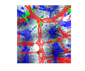
Exemplary instantaneous temperature and vertical velocity component fields are shown in figure 2. The instantaneous fields in figures 2(a) and 2(b) are obtained from measurements in the horizontal mid-plane at  ${Ra}=7 \times 10^{5}$, while those in figures 2(c) and 2(d) result from the DNS at
  ${Ra}=10^{6}$ at the same position. With respect to the measurement uncertainty, the field of view of the three cameras applied for the measurements has been adjusted, yielding the intersection of the experimentally determined temperature and velocity fields in figure 2. For better comparability, the numerical results are restricted to the same section of the horizontal mid-plane.

Figure 2. Visualization of the instantaneous (a–d) and corresponding time-averaged fields (e–h) of the temperature  $\tilde {T}$, and of the vertical velocity component
  $\tilde {u}_z$ in the mid-plane, obtained from the laboratory experiments (exp) for Rayleigh number
  ${{Ra}=7 \times 10^{5}}$ (a,b,e, f) and from the DNS (sim) for Rayleigh number
  ${Ra}= 10^{6}$ (c,d,g,h). The circles in (e)–(h) indicate local events with a strongly pronounced vertical velocity component despite a small deviation from the average temperature, as described in the text.
As it can be seen in figures 2(b) and 2(d), the Rayleigh–Bénard flow is characterized by strong spatial variations of  $\tilde {u}_z$ with upwellings and downwellings due to rising and falling thermal plumes. To some extent, the fingerprints of the flow can also be identified in the corresponding instantaneous temperature fields. However, one observes that larger areas with similar temperature ranges appear. A closer look reveals that these areas can also be detected in the instantaneous field of the vertical velocity component. This indicates that the flow not only exhibits structures at smaller length scales, but also tends to develop patterns at somewhat larger scales. As the small-scale flow structures rearrange quickly and display stronger temporal fluctuations, they can be removed effectively in both fields by time averaging. As a result, the large-scale patterns are revealed. The latter are denoted as turbulent superstructures and can be seen clearly in the time-averaged fields of the temperature and the vertical velocity component in figures 2(e–h).
In the evaluation of the experimental data, the full recording time of 5 min for each series of images has been taken as the time-averaging interval that translates into 125 free-fall units in the considered case with  ${Ra}=7 \times 10^{5}$. The numerical data have been evaluated according to Fonda et al. (Reference Fonda, Pandey, Schumacher and Sreenivasan2019), in which averaging times of 207 free-fall units and 179 free-fall units are given for
  ${Ra}=10^{5}$ and
  ${Ra}=10^{6}$, respectively. Hence, the experimental data are averaged over a somewhat shorter time interval. However, the quantitative analysis on the basis of the time-averaged fields in §§ 5 and 6 will not be affected by this slight difference, since the averaging time is sufficiently long to reveal clearly the turbulent superstructures (see also the supplementary information of Pandey et al. (Reference Pandey, Scheel and Schumacher2018)).
The comparison of the time-averaged temperature and velocity fields in figure 2 shows that the turbulent superstructures yield sharp contours in the vertical velocity component, while giving smoother contours of the temperature field. In addition, it can be anticipated without further analysis that the characteristic length scale in the temperature field is somewhat larger than in the velocity field. This behaviour was also found in the DNS by Pandey et al. (Reference Pandey, Scheel and Schumacher2018). The effect can be explained by the fact that at the onset of convection the temperature field and the vertical velocity field are perfectly synchronized (hot fluid dwells in the upward direction, whereas cold fluid sinks down), and thus show the same characteristic wavelengths in both fields. The synchronization decays with increasing Rayleigh number since the temperature field is not only advected by the vertical velocity component across the mid-plane, but also stirred by increasing velocity fluctuations in the horizontal directions. As a consequence, the contours of the superstructures in the temperature field might appear broader given the fact that the thermal plumes are dispersed by the velocity fluctuations when rising or falling into the bulk of the layer. Locally, this can lead to slight differences in the pattern scales of temperature and velocity fields. For example, this is visible around  $(\tilde {x},\tilde {y})=(6,7)$ in the experimental results and around
  $(\tilde {x},\tilde {y})=(15,16)$ in the numerical simulation, where the temperature is close to
  $\tilde {T}=0.5$ despite a strong vertical fluid motion in the upward or downward direction (see also circles in figure 2). However, the turbulent superstructures in the temperature and velocity fields can be found in good qualitative agreement. Visual inspection of the results indicates that the experimentally determined turbulent superstructures seem to be somewhat larger, which will be detailed in § 5.
Comparing the temperature fields in figure 2, it can also be seen that the occurring temperatures span a wider range in the experiment. This is confirmed by the standard deviation of the temperature  $\sigma _{T}$ in table 3. We suspect that this is an effect of the turbulent superstructures on the temperature distribution at the heating plate and the cooling plate in the experimental set-up, as the impinging superstructures yield some slightly warmer and colder regions on both plates. In contrast, the range of vertical velocity amplitudes is larger in the simulations, as is obvious from figure 2. A possible explanation for this observation is the higher spatial resolution of the DNS data. The in-plane resolution for the PIV measurements can be increased largely by advanced algorithms. For the current case, we obtained in-plane vector spacing of about
  $\Delta (\tilde {x},\tilde {y}) = 0.084$, for
  $Ra = 2 \times 10^5$ as well as
  $Ra = 4 \times 10^5$ and about
  $\Delta (\tilde{x}, \tilde{y}) = 0.056$ for
  $Ra = 7 \times 10^5$, corresponding to 2.35 mm and 1.57 mm, respectively. In the vertical direction, the resolution is given by the light sheet thickness, which amounts to 3–4 mm and cannot be improved further. It is this vertical resolution that limits the resolution in all spatial directions. Even though the experiment allows us to resolve most of the small-scale structures, the peak velocities embedded in the fine structures are not captured fully due to the spatial averaging of the velocity in the PIV measurements, such that the largest magnitudes are slightly smoothed out (Kähler, Scharnowski & Cierpka Reference Kähler, Scharnowski and Cierpka2012). However, the difference between the numerical and experimental results regarding the velocity range is smaller, as seen in figure 6 and table 3, where the root-mean-square velocity
  $U_{rms} = (\langle u_x^{2}+u_y^{2}+u_z^{2} \rangle )^{1/2}$ and the resulting Reynolds number
  ${Re}=({Ra}/{Pr})^{1/2}\,U_{rms}$ are also listed for each simulation and experiment.
Table 3. Results of the numerical and experimental investigations. The table lists the standard deviation of the temperature  $\sigma _T$, the root-mean-square velocity
  $U_{rms}$, the Reynolds number
  $Re$, the Nusselt number
  $Nu$ according to its definition (4.1), and the mean characteristic wavelength of the turbulent superstructures determined from the temperature field
  $\langle \hat {\lambda }_T \rangle$ and the field of the vertical velocity component
  $\langle \hat {\lambda }_{u_z} \rangle$. In the case of the DNS, the quantities are determined from the horizontal mid-plane for a better comparability with the experimental data. In addition, the temperature and velocity data of the DNS are re-computed in small interrogation volumes around the horizontal mid-plane to estimate the effect of the smaller spatial resolution of the experimental data. The quantities resulting from the coarse-grained grid are denoted as
  $\sigma _{T_{co}}$,
  $U_{{co},{rms}}$,
  ${Re}_{{co}}$ and
  ${Nu} _{{co}}$.

The root-mean-square velocities and Reynolds numbers of the DNS have also been computed on a coarser grid to investigate the effect of the smaller spatial resolution of the measurements. For this, the temperature and velocity data have been averaged in small interrogation volumes around the horizontal mid-plane. Hence, the numerical data have been averaged not only in the horizontal direction, but also to some extent in the vertical direction, thereby taking into account that the light sheet for the illumination of the measurement area has a certain thickness. The size of the interrogation volumes has been chosen such that the spatial resolution of the numerical data for  ${Ra}=10^{5}$ and
  ${Ra}=10^{6}$ roughly matches that of the experimental data for
  ${Ra}=2 \times 10^{5}$ and
  ${Ra}=7 \times 10^{5}$, respectively. The resulting root-mean-square velocities
  $U_{{co},{rms}}$ and Reynolds numbers
  ${Re}_{{co}}$ are also given in table 3. As expected, the magnitude of these quantities decreases due to the smaller spatial resolution. The numerical results are therefore fairly well in line with the experimental results.
4. Analysis of the local convective heat flux
The simultaneous measurement of the temperature and the vertical velocity component allows us to determine the local convective heat flux in RBC. Measurements of the local convective heat flux have been performed in the past, e.g. by tracking a mobile Lagrangian temperature sensor (Gasteuil et al. Reference Gasteuil, Shew, Gibert, Chillá, Castaing and Pinton2007). Shang et al. (Reference Shang, Qiu, Tong and Xia2004) combined laser-Doppler velocimetry and temperature probe measurements to determine time series of the components of the local convective heat flux vector as a function of the cell radius. It was found that the most significant flux contribution stems from the large-scale circulation that rises or sinks along the side walls. The novelty of the present study is that the local heat transfer is investigated as a field in the mid-plane in the Eulerian frame of reference. The Nusselt number  ${Nu}$ as the global measure of turbulent heat transfer is defined as
 \begin{equation} {Nu}(\tilde{z})=\sqrt{{Ra\,Pr }}\,\langle \tilde{u}_z\, \tilde{T}(z)\rangle_{A,t} - \dfrac{\partial \langle \tilde{T}(z)\rangle_{A,t}}{\partial z} ={\rm const}. \end{equation}
Recall that  ${Nu}(\tilde {z})$ takes the same value for any
  $0\leqslant \tilde {z}\leqslant 1$, even though the contributions to the heat transfer due to convective fluid motion (conv) and diffusion (diff) differ near the boundaries compared to those in the bulk; see e.g. Scheel & Schumacher (Reference Scheel and Schumacher2014). At the horizontal mid-plane, the second term in equation (4.1) is zero in the Boussinesq regime with its top-down symmetry. In dimensionless units, the two corresponding local currents are given by
 \begin{equation} J_{conv}(\tilde{\boldsymbol{x}}, \tilde{t})=\sqrt{{Ra\,Pr }}\, j_z(\tilde{\boldsymbol{x}}, \tilde{t})=\sqrt{{Ra\,Pr }}\, \tilde{u}_z(\tilde{\boldsymbol{x}}, \tilde{t})\, \tilde{T}(\tilde{\boldsymbol{x}},\tilde{t}) \end{equation}
and
 \begin{equation} J_{diff}(\tilde{\boldsymbol{x}},\tilde{t})={-}\frac{\partial \tilde{T}(\tilde{\boldsymbol{x}},\tilde{t})}{\partial \tilde{z}}. \end{equation}
Since  $0\leqslant \tilde {T}\leqslant 1$, we take a symmetric form that is obtained by decomposing the original temperature field into the linear diffusive equilibrium profile and the rest:
 \begin{equation} \tilde{T}(\tilde{\boldsymbol{x}},\tilde{t}) = 1-\tilde{z} + \tilde{\varTheta}(\tilde{\boldsymbol{x}},\tilde{t}). \end{equation}
Thus we define eventually a local convective Nusselt number at  $\tilde {z}=1/2$ by
 \begin{equation} {Nu}_{loc}(\tilde{x},\tilde{y},\tilde{t})=\sqrt{{Ra}\,{Pr}}\,\tilde{\varTheta}(\tilde{x},\tilde{y},\tilde{t})\,\tilde{u}_z(\tilde{x}, \tilde{y}, \tilde{t}), \end{equation}
which is accessible directly as a field in the experiments. The uncertainty for the temperature measurements of 0.1 K results in an uncertainty for the individual values of the Nusselt number of about 14 % for  $Ra = 2 \times 10^{5}$, 7 % for
  $Ra = 4 \times 10^{5}$, and 4 % for
  $Ra = 7 \times 10^{5}$. However, the mean values (see table 3) show a much lower uncertainty as
  ${\sim} 216 \times 10^6$ data points for the two lower Rayleigh numbers and
  ${\sim} 483 \times 10^6$ data points for the highest Rayleigh number are averaged.
An exemplary instantaneous field of the local convective Nusselt number, which has been determined from figures 3(a) and 3(b), is depicted in figure 3(c). These results of the measurement at  ${Ra}=2 \times 10^{5}$ already indicate the effect of the superstructures on the local convective heat flux, which appears even clearer in the corresponding time-averaged fields in figures 3(d), 3(e) and 3( f). It can be seen that the maximum values of the local convective Nusselt number occur in the regions, where the time-averaged temperature reaches its extreme values, corresponding to updrafts and downdrafts of the turbulent superstructures. It is therefore confirmed that the superstructures strongly enhance the heat flux from the bottom to the top of the Rayleigh–Bénard cell. It can also be seen that multiple regions of strong heat transfer develop that are distributed homogeneously over the whole field of view. These regions are not constrained by the side walls, which is different to Rayleigh–Bénard convection experiments in small-aspect-ratio cells (Shang et al. Reference Shang, Qiu, Tong and Xia2004).

Figure 3. Exemplary instantaneous and the corresponding time-averaged fields of the temperature (a,d), the vertical velocity component (b,e), and the local Nusselt number (c, f), obtained from the measurement in the mid-plane at Rayleigh number  ${{Ra} = 2 \times 10^{5}}$. The fields are computed as
  $\tilde {T} = (T-T_{c})/(T_{h}-T_{c})$,
  $\tilde {u}_z = u_z/\sqrt {h g \alpha \, \Delta T}$ and
 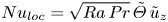 ${Nu}_{loc} = \sqrt {{Ra}\,{Pr}} \,\tilde {\varTheta }\,\tilde {u}_z$. The circles in (a)–(c) indicate exemplary events with a negative local Nusselt number, i.e. the heat is transferred towards the heating plate as outlined in the text.
The quantitative analysis of the local heat flux is done by the probability density functions (p.d.f.s) of the local convective Nusselt number as shown in figure 4(a) for each of the three measurements, and in figure 4(b) for the two DNS cases. Here, the p.d.f.s incorporate all the temporally resolved values obtained from the measurements and the DNS at each Rayleigh number. As expected, the p.d.f.s are more extended for positive values, since the total heat transfer increases due to convective motion. It can also be seen that the negative tails increase with the Rayleigh number, which shows that in turbulent thermal convection the upward motion of cold fluid and the downward motion of warm fluid become more probable.

Figure 4. The probability density functions of the temporally resolved local convective Nusselt number resulting from the measurements in the mid-plane (a) and from the DNS (b).
The data also allow us to evaluate the probability density functions of the normalized vertical convective heat current component  $j_z/j_{z,{rms}}$, as shown in figure 5(a) for each of the three measurements, and in figure 5(b) for the two DNS cases. Shang et al. (Reference Shang, Qiu, Tong and Xia2004) performed the same analysis and showed for a
  $\varGamma = 1$ cell that the p.d.f.s fall on top of each other for a Rayleigh number range from
  $Ra = 1.8\times 10^{9}$ to
  $Ra = 7.6 \times 10^{9}$. The present p.d.f.s of the normalized vertical convective heat current are supported on a similar interval (see figure 9 of Shang et al. Reference Shang, Qiu, Tong and Xia2004). The p.d.f.s are also skewed to positive values since a mean heat flux goes from the bottom to the top. It can also be seen now that the positive tails on both panels collapse fairly well onto each other, for both experiments and simulations. However, the negative tails still differ despite being closer compared to figure 4. This effect is again attributed to the non-ideal boundary conditions that hinder the fast heat transport by conduction in the top plate. This effect becomes more dominant with increasing Rayleigh numbers, as will be outlined below.

Figure 5. The probability density functions of the fluctuations of the vertical convective heat current component normalized by the corresponding root-mean-square value. These data result from the measurements in the mid-plane (a) and from the DNS (b). Data are the same as in figure 4.
In order to compare further the experimental and numerical results regarding the heat flux, the spatial and temporal averages of the local convective Nusselt number  ${Nu}_{loc}$ are plotted in figure 6. Even though the contribution of the diffusive heat flux cannot be obtained from the experimental data, the resulting average of the convective flux with respect to time and area is representative for the total heat flux, since the observation area in the experiment is large enough. By applying the power-law fit of
  ${Nu}=0.133\times Ra^{0.298}$ (see red dashed line in figure 6a), which has been obtained from DNS for three Rayleigh numbers,
  ${Ra}=10^{5}$,
  $10^{6}$ and
  $10^{7}$ (Fonda et al. Reference Fonda, Pandey, Schumacher and Sreenivasan2019), one gets
  ${Nu}=5.11$,
  $6.37$ and
  $7.44$ for the three Rayleigh numbers of the experimental series. Hence, the global Nusselt number as determined from the experiments according to table 3 is on average about 25 % smaller than expected on the basis of the numerical results. Despite these deviations in magnitude, the scaling exponent of the global heat transfer power law can be considered as similar to the DNS. A power-law fit of
  ${Nu}=0.121\times Ra^{0.286}$ results from the experimental data (see black dashed line in figure 6a).

Figure 6. Nusselt number versus Rayleigh number (a), and Reynolds number versus Rayleigh number (b). Values are taken from table 3 for the numerical results for the coarse-grained data.
An underestimation of the total heat transfer in the experiment is possible, because the temperature and the velocity are measured with a lower spatial resolution and can also be considered as an average across the thickness of the light sheet used for the illumination of the tracer particles. The effect of these two aspects can be shown easily by means of the data of the numerical simulations. For this, the temperature and the vertical velocity component are averaged in small interrogation volumes around the horizontal mid-plane as has been described in § 3 for the estimation of the root-mean-square velocity  $U_{{co},{rms}}$ and the Reynolds number
  ${Re} _{{co}}$. If the coarse-grained temperature and the vertical velocity fields are applied to compute the global Nusselt number
  ${Nu} _{{co}}$ from the DNS data, then the values converge to the experimentally determined Nusselt number
  $Nu$ according to the results in table 3.
However, as the Nusselt numbers show, the convective heat flux in the experiment is still smaller in comparison to the simulations. This aspect may be attributed to the boundary conditions. In the numerical simulations, perfect isothermal boundary conditions can be set, while temperature inhomogeneities at the boundaries cannot be impeded fully in an experiment. A dimensionless measure of the uniformity of the prescribed temperature at the boundaries is the Biot number (Verzicco Reference Verzicco2004; Schindler et al. Reference Schindler, Eckert, Zürner, Schumacher and Vogt2022), which is given by
 \begin{equation} {Bi} = {Nu}\left(\frac{k_{f} h_{w}}{k_{w} h}\right), \end{equation}
with  $k_{f}$,
  $h$ and
  $k_{w}$,
  $h_{w}$ being the heat conduction coefficient and the thickness of the fluid layer and the wall material, respectively. The Biot number can also be interpreted as the ratio of the thermal resistance due to thermal conduction in the wall and the thermal resistance due to convective heat transfer at the wall. If
  ${Bi}\ll 1$, then the limiting heat transfer mechanism is the convective heat transfer and not the conduction within the wall material, such that the isothermal boundary condition can be assumed.
For the heating plate made of aluminium, the Biot number is of the order  ${Bi} \sim 10^{-3}$ and thus is sufficiently small. However, the cooling plate is made of glass for the optical access. The glass plate has a thickness of
  $h_{\rm w} =8$ mm and a thermal conductivity of
  $k_{w} = 0.78\ {\rm W}\ {\rm m\ K}^{-1}$. Assuming
  $k_{f} = 0.6\ {\rm W}\ {\rm m\ K}^{-1}$ for the thermal conductivity of water at the mean fluid temperature of about
  $T=20\,^{\circ }{\rm C}$, the Biot number increases with the Rayleigh numbers adjusted in the experiment from
  ${Bi} = 0.86$ to
  ${Bi} = 1.22$. Therefore, the thermal resistance due to conduction in the wall is not negligible in this case, and limits the heat transfer. A transparent material with a much higher thermal conductivity would be sapphire. However, such a sapphire plate of dimensions
  $70 \times 70\ {\rm cm}^{2}$ is not available off the shelf and would have to be produced individually as a growing aluminium-oxide monocrystal. Therefore, we had to stick with the non-ideal boundary conditions. Hot plumes from the bottom cannot transfer their thermal energy to the top plate in the same way as for the case of an isothermal boundary condition in the simulation. Due to continuity, the flow is forced to move downwards with higher temperatures. This results in more events with a negative local convective Nusselt number, as is obvious from figure 4(a), where the correspondence between experiment and simulation is good for positive values of the local convective Nusselt number, but differs for negative ones. The occurrence of events transferring heat towards the heating plate can be seen clearly in figure 3(c) in the form of blue regions, which correspond to hot fluid streaming downwards, for example at
  $(\tilde {x},\tilde {y}) \approx (14, 16)$, and cold fluid that moves upwards, for example at
  $(\tilde {x},\tilde {y}) \approx (4, 9)$, indicated by the circles in figures 3(a–c).
Due to the limitation of the convective heat transfer, which results from the material properties of the top plate, the local convective Nusselt number in the experiment is on average smaller than in the simulation, which is also visible by the larger positive tails for the DNS data in figure 4. The difference for the mean value increases with the Rayleigh number, as the resistance for heat conduction in the top plate remains constant, while the turbulent convective heat transfer increases, and thus the Biot number increases as well. In the present case, the ratio of the Nusselt number obtained from the DNS and from the experiment is of the same order as the Biot number, i.e.  ${Nu}/{Nu}_{exp} \sim {Bi}$. This effect would also explain the smaller velocities in the experiment, as the driving of the flow is hampered. Moreover, Vieweg, Scheel & Schumacher (Reference Vieweg, Scheel and Schumacher2021a) found that the variance of the temperature in the mid-plane is two orders of magnitude larger in the case of constant heat flux compared to the case of constant temperature at the horizontal boundaries. This result is obtained by P.P. Vieweg through an additional analysis of simulation data published in Vieweg et al. (Reference Vieweg, Scheel and Schumacher2021a). The finding is in line with the larger standard deviation of the temperature
  $\sigma _{T}$ for the experimental data according to table 3.
5. Characteristic length scale of turbulent superstructures
The visual comparison of the temperature and velocity fields in figure 2 already indicates that turbulent superstructures in the experiments have a somewhat larger horizontal length scale than in the numerical simulations. For the quantitative estimation of the size of the superstructures in the experiment, the temperature field is considered in the following. As described in Pandey et al. (Reference Pandey, Scheel and Schumacher2018), the size of the superstructures can be determined via Fourier spectral analysis on the basis of the field  $\tilde {\varTheta }$, which represents the temperature difference to the linear diffusive equilibrium profile at the height of the measurement plane. For simplicity, this field is denoted as the temperature field from here on. The characteristic horizontal length scale of the superstructures can be derived from the so-called power spectrum, which represents quantitatively the match between the temperature field and sinusoidal plane waves with different wavelengths and orientations.
A power spectrum of an exemplary time-averaged temperature field depicted in figure 7(a) can be seen in figure 7(b). Here, the power spectrum  $P_{\tilde {\varTheta }}$ is arranged in a way such that the dimensionless wavenumber
  $\tilde {k}=(\tilde {k}_x,\tilde {k}_y)$ increases from the centre towards each of the edges. Hence, the entries of the power spectrum on the same circumference around the centre represent features with the same wavenumber but a varying orientation. It shall also be noted that the power spectrum is symmetric around the centre, such that
  $P_{\tilde {\varTheta }}\,(k_x,k_y)=P_{\tilde {\varTheta }}\,(-k_x,-k_y)$. Due to the time averaging, the turbulent superstructures represent the prominent pattern in the temperature field, which is also obvious from the two distinctive maxima of the power spectrum. These two symmetric maxima occur, since the superstructures are in this case arranged preferentially along a certain direction, namely along the line connecting the two maxima. However, the superstructures do not exhibit a preferential orientation for all data records along a specific direction. In some cases, they are also represented by a ring-like structure of enhanced spectral power rather than two prominent maxima. Therefore, the azimuthal average of the power spectrum can be taken to determine the circumference with the largest average, in order to identify the characteristic wavelength of the superstructures. For a better visualization of the length scales, the average intensities
  $I_\lambda$ normalized with the maximum are shown in figure 7(c) in dependence on the dimensionless wavelength
  $\tilde {\lambda }=\lambda /h$. The latter is related to the wavenumber via
  $\tilde {\lambda }=2{\rm \pi} /\tilde {k}$.

Figure 7. Procedure for the determination of the characteristic wavelength of the turbulent superstructures. (a) An exemplary time-window averaged temperature field  $\tilde {\varTheta }$. (b) The corresponding power spectrum
  $P_{\tilde {\varTheta }}$. (c) The normalized wavelength intensities of the power spectrum determined from the original temperature field
  $\tilde {\varTheta }$ and from the filtered temperature field
  $\tilde {\varTheta }\rvert _{\forall \,\lvert \tilde {k}\rvert \geqslant 0.4}$. The latter is shown in figure 8(a).
As the grey curve shows, there are two distinctive local maxima. While the peak at  $\tilde {\lambda } \approx 8.7$ represents the superstructures, the peak at
  $\tilde {\lambda } \approx 29$ results from the experimental boundary conditions. The second peak corresponds to the vertically aligned maxima close to the centre in figure 7(b), and can be explained by the increasing temperature of the cooling water in its flow direction from the bottom to the top edge in figure 7(a). A closer look at this figure reveals that the measured temperature fields also exhibit the trend of larger temperatures along the cooling water flow in
  $y$-direction due to the slight increase of the cooling water temperature, which amounts to
  $\Delta T_{cw,y} \leqslant 0.15\ {\rm K}$. In order to ensure that the characteristic wavelength of the superstructures is not determined based on the wrong maximum in any case, the large-scale trend is removed from the time-averaged temperature fields by computing the inverse Fourier transform without considering the smallest wavenumbers close to the centre of the power spectrum, meaning that the corresponding Fourier coefficients are set to zero. The limit of the wavenumber
  $\tilde {k}=(\tilde {k}_x^{2}+\tilde {k}_y^{2})^{1/2}=0.4$ has been chosen, such that all the wavelengths
  $\tilde {\lambda } > 2{\rm \pi} /0.4=15.7$ are not taken into account. The latter span much wider horizontal dimensions compared to the turbulent superstructures. On the basis of the temperature field with the removed large-scale trend, which is depicted in figure 8(a), the procedure for the determination of the average intensities
  $I_\lambda$ is then performed again. The resulting wavelength intensities with a clear peak at the characteristic wavelength of the superstructures can be seen also in figure 7(c). This confirms the applicability of the filtering approach.

Figure 8. Exemplary demonstration of the reorganization of the turbulent superstructures by means of two time-averaged temperature fields in the mid-plane at Rayleigh numbers  ${Ra}=2 \times 10^{5}$ (a,d),
  ${Ra}=4 \times 10^{5}$ (b,e), and
  ${Ra}=7 \times 10^{5}$ (c, f).
In the evaluation of the numerical data, such a filtering is not required, because there are no deviations from the isothermal boundary condition yielding a large-scale trend of the temperature. Therefore, the power spectrum obtained from the time-averaged temperature field can be applied directly to derive the characteristic wavelength of the superstructures from the position of the maximum azimuthal average. The mean characteristic wavelengths of the superstructures  $\langle \hat {\lambda }_T \rangle$, obtained from the experimental and numerical investigations, are given in table 3. At each Rayleigh number, the 19 time-averaged temperature fields resulting from the image series covering 5 min have been considered to determine
  $\hat {\lambda }_T$ for the experiment, while sliding time averages in the total runtime of the simulations have been used to calculate
  $\hat {\lambda }_T$ for the DNS. The total runtimes and the number of equidistantly stored sliding time averages are given in Fonda et al. (Reference Fonda, Pandey, Schumacher and Sreenivasan2019).
For the estimation of the characteristic wavelength of the superstructures, the time-averaged field of the vertical velocity component has been considered, too. In principle, the resulting wavelengths  $\langle \hat {\lambda }_{u_z} \rangle$ according to table 3 are obtained in the same way as for the temperature field, but the filtering approach of the experimentally determined velocity field has been changed slightly. It is obvious from figure 3(e) that some regular variations of the vertical velocity component remain on small length scales after the time averaging. Thus the filtering has been modified such that variations of the velocity on either much larger or smaller length scales compared to the turbulent superstructures are removed. The wavelengths in the range
  $4.8 \leqslant \tilde {\lambda }_{u_z} \leqslant 15.7$ are not affected by the filtering. However, despite the additional filtering of small-scale variations of the velocity, the characteristic wavelengths determined from the time-averaged velocity field are somewhat smaller than those of the temperature field according to table 3. This is also the case for the fields obtained from the DNS, which might be caused by the time averaging.
The results in table 3 show that the characteristic wavelength of the superstructures  $\langle \hat {\lambda }_T \rangle$ increases with the Rayleigh number according to the experiments, while the wavelength remains nearly constant according to the DNS. Moreover, the characteristic wavelengths determined from the DNS are typically one-third smaller. Considering the boundary conditions of the experiment, this is also reasonable. Due to thick insulation around the side wall of the cell and the adaption of the temperature in the lab to the mean temperature of the working fluid, the adiabatic boundary condition at the side wall is well satisfied, but deviations from the isothermal boundary condition at the horizontal plates cannot be fully impeded in an experimental set-up. Despite extensive efforts in the experimental set-up at hand, especially the top plate made of glass for optical accessibility cannot compensate the effect of the impinging flow structures without a temporal delay.
Based on the above discussion of the Biot number and on theoretical considerations (Hurle, Jakeman & Pike Reference Hurle, Jakeman and Pike1967), it can be shown that the limited thermal conductivity of the plates enclosing the fluid layer alters strongly the flow in comparison to the classical RBC with isothermal boundary conditions. In this respect, the ratio of the effective thermal conductivity of the working fluid  $k_{f}$ to the thermal conductivity of the solid plates
  $k_{w}$ is essential. The two extreme cases
  $k_{f}/k_{w} \rightarrow 0$ and
  $k_{f}/k_{w} \rightarrow \infty$, which correspond to the Dirichlet boundary condition with constant temperature at the plates and the Neumann boundary condition with constant heat flux at the plates, have been compared in the study by Vieweg et al. (Reference Vieweg, Scheel and Schumacher2021a) on the basis of DNS for
  $\varGamma =60$. While the first case yields the turbulent superstructures with a horizontal extent larger than the height of the cell, the second case results in structures that grow gradually and aggregate to one large structure spanning even the entire flow domain. Neither of these extreme cases is matched perfectly in any experiment; however, here the temperature at the bottom plate is almost uniform due to the high thermal conductivity of aluminium and
  $k_{f}/k_{w} \ll 1$. At the top plate, which is made of glass, this ratio is
  $k_{f}/k_{w} \approx 1$ when taking into account that the effective thermal conductivity of the fluid increases due to the convective motion. Therefore, the increase of the horizontal characteristic scale of the superstructures in comparison to the DNS might be caused by non-ideal boundary conditions at the cooling plate that are a mixture of constant temperature and constant heat flux.
6. Long-term evolution of the turbulent superstructures
Compared to the data of the DNS, which are often limited to total simulation times of several hundred free-fall units, the experimental data span approximately  $5\times 10^{3} t_{f}$ up to
  $10^{4} t_{f}$ free-fall units for the different Rayleigh numbers. Hence the ability to run the experiments over long time intervals offers the possibility of evaluating the reorganization of the turbulent superstructures, which can be seen in figure 8, showing two different time-averaged temperature fields in the horizontal mid-plane for the different Rayleigh numbers adjusted in the experiments. The time difference between these two temperature fields is 200 min, which corresponds to
  $2663 t_{f}$ at
  ${Ra}=2 \times 10^{5}$, to
  $3846 t_{f}$ at
  ${Ra}=4 \times 10^{5}$, and to
  $4988 t_{f}$ at
  ${Ra}=7 \times 10^{5}$. The differences in the distribution of warm and cold regions in the temperature field demonstrate the relocation of the superstructures.
On the basis of the numerical studies by Pandey et al. (Reference Pandey, Scheel and Schumacher2018) and Fonda et al. (Reference Fonda, Pandey, Schumacher and Sreenivasan2019), it can be estimated that the turbulent superstructures in water reorganize every 200 free-fall units on average, if the Rayleigh number is in the range  $10^{5} \leqslant {Ra} \leqslant 10^{6}$. In order to assess the gradual long-term evolution of the superstructures, for each time-averaged field obtained from one of the 19 series of 1500 snapshots, the central coefficient of the normalized two-dimensional cross-correlation is calculated according to
 \begin{equation} R_{\alpha\alpha}(\tilde{t}_0, \Delta\tilde{t})=\frac{\langle (\bar{\boldsymbol{\mathsf{X}}}_{\alpha}(\tilde{t}_0)-{\boldsymbol{\mathsf{\mu}}}_{\bar{\boldsymbol{\mathsf{X}}}_{\alpha}(\tilde{t}_0)})(\bar{\boldsymbol{\mathsf{X}}}_{\alpha} (\Delta\tilde{t})-{\boldsymbol{\mathsf{\mu}}}_{\bar{\boldsymbol{\mathsf{X}}}_{\alpha}(\Delta\tilde{t})})\rangle}{\sigma_{\bar{X}_{\alpha}( \tilde{t}_0)}\sigma_{\bar{X}_{\alpha}(\Delta\tilde{t})}} \quad \mbox{with}\ \Delta\tilde{t}=i\tilde{t}_{rec}. \end{equation}
Here, the running index is  $i \in [0,18]$, and
  $\tilde {t}_{rec}=t_{rec}/t_{f}$ is the dimensionless time interval between each of the 19 image series, with
  $t_{rec}=20\ {\rm min}$ as given in § 2.1. The Greek symbol
  $\alpha$ represents the quantities
  $\alpha =\{\tilde {T}, \tilde {u}_z, {Nu_{loc}}\}$,
  $\bar {\boldsymbol{\mathsf{X}}}_{\alpha }$ are the respective time-averaged dimensionless fields, and
  ${\boldsymbol{\mathsf{\mu}}} _{\bar {\boldsymbol{\mathsf{X}}}_{\alpha }}$ and
  $\sigma _{\bar {X}_{\alpha }}$ are the corresponding mean value and standard deviation, respectively. Furthermore,
  $\langle \cdot \rangle$ denotes the average. This analysis shows that for all Rayleigh numbers the temporal variation of the time-averaged temperature fields is not as pronounced as the variation of the time-averaged fields of the vertical velocity component and the local Nusselt number. If two successive time-averaged temperature fields are considered, respectively, then the correlation coefficient remains on a high level of
  $R_{\tilde {\varTheta }\tilde {\varTheta }} \approx \{0.5, 0.7, 0.8\}$ for
  $Ra = \{2 \times 10^{5}, 4 \times 10^{5}, 7 \times 10^{5}\}$. Again, this behaviour can be attributed to the boundary conditions, as the deviation from the isothermal boundary condition at the top wall becomes stronger with increasing Rayleigh number. If the temperature value at the top plate is at a certain point larger than in the neighbourhood due to an impinging superstructure, then this causes a stabilization of the superstructure at that position, such that a random reorganization of the structures will take longer or is inhibited. In order to analyse the gradual reorganization, the time-averaged fields of the temperature, vertical velocity component and local Nusselt number for
  ${Ra}=2 \times 10^{5}$ are evaluated, as the dimensionless temporal delay between each of the fields is the smallest for this Rayleigh number and amounts to about
  $\tilde {t}_{rec}=266$. The correlation coefficients have been normalized for this purpose and are shown in figure 9.

Figure 9. Time correlation coefficient  $R_{\alpha \alpha }$ for the experimental data obtained from the measurement at
  ${Ra}=2 \times 10^{5}$. The typical time scales were estimated at a normalized correlation coefficient
  $R_{\alpha \alpha }=1/{\rm e}$, which is indicated with the horizontal dashed line.
Based on the normalized correlation coefficients, the typical time scales for the rearrangement of the superstructures are estimated to be  $\tau _{\tilde {T}} \approx 920$,
  $\tau _{\tilde {u}_z} \approx 320$ and
  $\tau _{{{Nu_{{loc}}}}} \approx 200$ for the fields of the temperature, the vertical velocity component and the local Nusselt number, respectively. This confirms the aforementioned finding that in the present case, the temperature patterns persist much longer in comparison to the characteristic patterns of the velocity field and of the corresponding local Nusselt number field. In order to investigate further the reorganization of the turbulent superstructures, and evaluate their role in heat transfer, a spatial and temporal median filter with kernel size
  $n_{\tilde {x}} \times n_{\tilde {y}} \times n_{\tilde {t}} = 9 \times 9 \times 3$ was applied to the total data. In the smoothed fields of the temperature, the vertical velocity component and the local Nusselt number isosurfaces can be extracted that display the reorganization in time effectively.
Space–time isosurfaces of the time-averaged temperature field are shown for  $\bar {X}_\varTheta = \pm 0.13$ in figure 10(a), and of the time-averaged vertical velocity component field for
  $\bar {X}_{u_{z}} = \pm 0.025$ in figure 10(b). Both fields are replotted in figures 10(c,d) as a view from the top. In addition, isosurfaces of
  $\bar {X}_{Nu_{loc}} = 0$ are superposed in green within the panels showing the velocity isosurfaces. It is seen that the temperature field contours change gradually due to a certain reorganization of the superstructures. The isosurfaces bifurcate partly or end in the course of the time evolution. Furthermore, the isosurfaces of the vertical velocity component in figures 10(b,d) vary much more strongly in space and time, as can be expected on the basis of the correlation coefficients in figure 9. In the view from the top, it can now be seen clearly that cells of strongly downwelling fluid in the middle (blue) and upwelling fluid in a kind of rim (red) do form. Even though these patterns remain relatively stable, especially for the case of the upwelling fluid, a variation of the orientation of the ridges becomes apparent. These patterns do not necessarily coincide with the region of a larger temperature magnitude, which explains the decreased average of the local Nusselt number and the larger portion of negative local Nusselt numbers in the experiments, as is obvious from table 3 and figure 4. It is interesting to note that regions with negative local Nusselt numbers also remain for a certain time
  $\tilde {t} \sim {{O}}(10^{3})$.

Figure 10. Isosurfaces of  $\tilde {\varTheta }$ (a,c), as well as of
  $\tilde {u}_{{z}}$ and
  ${Nu}_{{loc}}$ (b,d), for the experimental data obtained from the measurement at
  ${Ra}=2 \times 10^{5}$. Panels (c,d) show the isosurfaces from the top view.
A more detailed look at one event with heat transfer towards the bottom plate can be seen in figure 11. In figure 11(a), a region with the temperature below the mean temperature is displayed. It is visible for  $\tilde {t} \in [1000, 3500]$. If at the same time the vertical velocity points downwards, then the local Nusselt number is positive. However, in figures 11(b,d), it can be seen in the isosurfaces of the vertical velocity component, that at a certain time instant, the velocity points upwards and thus colder fluid will be transported towards the cooling plate. In this case, the local Nusselt number becomes negative, indicated by the green isosurface of the local Nusselt number for
  $\tilde {t} \in [2500, 3500]$. Later, the velocity still points upwards but the structures in the temperature field have reorganized and the local temperature is no longer colder than the mean temperature, such that the Nusselt number becomes positive again. From the current data it seems that this is a process that can be detected more often in the vicinity of the upwelling ridges. To summarize, a gradual evolution of the turbulent superstructures is observable clearly, as our space–time analysis suggests.

Figure 11. Isosurfaces of  $\tilde {\varTheta }$ (a,c), as well as of
  $u_{{z}}$ and
  ${Nu}_{{loc}}$ (b,d), in sections covering
  $\Delta \tilde {x} \times \Delta \tilde {y}= 4 \times 4$ (a,b) and
  $\Delta \tilde {x} \times \Delta \tilde {y}= 2 \times 2$ (c,d) for the experimental data obtained from the measurement at
  ${Ra}=2 \times 10^{5}$.
7. Conclusion and outlook
In this work, the structure and evolution of turbulent superstructures in a horizontally extended Rayleigh–Bénard convection layer have been investigated in a controlled laboratory experiment. Particle image velocimetry and thermometry were combined for the measurements in a water-filled Rayleigh–Bénard cell with dimensions  $l \times w \times h = 700\ \mathrm {mm} \times 700\ \mathrm {mm} \times 28\ \mathrm {mm}$. The aspect ratio is
  $\varGamma =l/h=25$, the Prandtl number is
  ${Pr}=7$, and the range of Rayleigh numbers is
  $2\times 10^{5}\leqslant Ra\leqslant 7\times 10^{5}$; thus the experimental results are comparable directly with existing results of direct numerical simulations. Here, we accessed the field structure of the three velocity components and the temperature in their joint dynamical evolution in a wider observation area of about
  $451\ \mathrm {mm} \times 468\ \mathrm {mm}$ centred in the bulk of the cell to study the spatiotemporal organization of the turbulent heat transfer. Due to its transparent side walls and the transparent cooling plate made of glass, the experimental set-up provides full optical access to the turbulent flow. Simultaneous measurements of the temperature and velocity fields in a large section of the horizontal mid-plane of the cell are thus feasible using thermochromic liquid crystals as tracer particles. Based on their temperature-dependent colour shade, the temperature field has been determined, while their temporal displacement has been evaluated to calculate both the horizontal and vertical components of the velocity field in the observation plane.
The time-averaged fields of the temperature and the vertical velocity component, obtained from the present experiments and the DNS, display clearly turbulent superstructures of convection, and agree qualitatively well. However, quantitative differences between the experimental and numerical results, in particular with respect to the characteristic wavelength of the large-scale patterns and the magnitude of the global Nusselt number, have been found. While the characteristic length scales of the turbulent superstructures are larger in the experiment, the values of the Nusselt number  ${Nu}$ are smaller compared to the results of the DNS. Both can be traced back to the deviations from the ideal isothermal boundary conditions at the top plate of the convection cell, which we discussed in detail in the text by an estimation of the corresponding Biot numbers. Despite the slight differences in the magnitude of the Nusselt number, the power-law exponent of the transport law
  ${Nu}({Ra})$ is in the same range as those of the DNS and other studies of thermal convection in water (Ahlers et al. Reference Ahlers, Grossmann and Lohse2009; Chillà & Schumacher Reference Chillà and Schumacher2012).
The joint measurement of the temperature and the vertical velocity component has been applied to study the local convective heat flux in the experiment, thereby demonstrating clearly that the skeleton of turbulent superstructures contributes significantly to the turbulent heat transfer from the bottom to the top of the cell. The contribution of the turbulent superstructures to the heat flux is therefore quantified by means of the local convective Nusselt number, which reaches its maxima within the localized updrafts and downdrafts that comprise the superstructure patterns in the flow.
Since the measurements of the temperature and velocity fields cover up to approximately  $10^{4}$ convective free-fall times, our investigations also allow us to study the reorganization of the superstructures for the different Rayleigh numbers. Their rearrangement is analysed here by means of the correlation coefficient of the time-averaged temperature fields. It is seen that the superstructures in the experiment have a preferential arrangement, most probably due to the slightly inhomogeneous temperature at the horizontal top plate. Nevertheless, the superstructures exhibit a clear gradual reorganization, which is in good agreement with the findings obtained in the previous numerical studies by Pandey et al. (Reference Pandey, Scheel and Schumacher2018) and Fonda et al. (Reference Fonda, Pandey, Schumacher and Sreenivasan2019).
Despite the non-ideal boundary conditions at the top plate, the presented results prove the concept of an experimental study of the long-term evolution of turbulent superstructures in Rayleigh–Bénard convection. A further improvement of the thermal boundary condition at the top plate of the experimental facility is one point for our future work. An alternative approach to the determination of the structures, which are connected to the local convective heat flux, would be volumetric velocity measurements of all three velocity components in a small volume. Again, these measurements would have to be combined with temperature measurements using TLCs and require a larger number of simultaneously operating cameras. These studies are currently underway and will be reported elsewhere.
Acknowledgements
The authors wish to thank A. Thieme and J. Fokken for the technical support in the laboratory, and P.P. Vieweg for discussions and the additional analysis of his simulation data.
Funding
Funding of this work by the Deutsche Forschungsgemeinschaft (DFG) within the Priority Programme DFG-SPP 1881 ‘Turbulent Superstructures’ and by the Carl Zeiss Foundation within project no. P2018-02-001 ‘Deep Turb–Deep Learning in and of Turbulence’ is acknowledged.
Declaration of interests
The authors report no conflict of interest.


 Open access