2. Mathematical modelling

The model formulation we use here is based on continuum mechanics and mixture theory where at each point in space and time in the porous material one can define phase volume fractions, along with field variables such as velocity and pressure. The model invokes averaging in the sense that a single point in space represents a small elemental volume in which all three phases – solid, liquid and gas – may be present in some proportion. This approach has been used extensively, especially in the context of flows in deformable porous materials, and builds on the pioneering work of Biot (Reference Biot1941a,Reference Biotb,Reference Biotc) with applications in biomechanics (e.g. Holmes Reference Holmes1983,  Reference Holmes1984,  Reference Holmes1985; Holmes & Mow Reference Holmes and Mow1990; Lai, Hou & Mow Reference Lai, Hou and Mow1991; Barry & Aldis Reference Barry and Aldis1993,  Reference Barry and Aldis1997) infiltration (e.g. Preziosi, Joseph & Beavers Reference Preziosi, Joseph and Beavers1996; Sommer & Mortensen Reference Sommer and Mortensen1996; Michaud, Sommer & Mortensen Reference Michaud, Sommer and Mortensen1999; Ambrosi & Preziosi Reference Ambrosi and Preziosi2000; Billi & Farina Reference Billi and Farina2000) printing (e.g. Chen & Scriven Reference Chen and Scriven1990; Fitt et al. Reference Fitt, Howell, King, Please and Schwendeman2002; Anderson Reference Anderson2005) and capillary-driven imbibition in various contexts (e.g. Siddique et al. Reference Siddique, Anderson and Bondarev2009; Siddique & Anderson Reference Siddique and Anderson2011; Anderson & Siddique Reference Anderson and Siddique2013; Mirnyy et al. Reference Mirnyy, Clausnitzer, Diersch, Rosati, Schmidt and Beruda2013).

The configuration of interest is one-dimensional capillary rise in a rigid porous material as outlined below. This is a common experimental configuration with available data and theory with which we can compare our work (e.g. Delker et al. Reference Delker, Pengra and Wong1996; Lago & Araujo Reference Lago and Araujo2001; Kim et al. Reference Kim, Ha and Kim2017). In the configuration of interest shown in figure 1, a reservoir supplies fluid at the bottom of the porous material, $z=0$ at time $t=0$, one interface position, $z=h_{\ell }^S(t)$, marks the top of the fully saturated region which occupies $0 < z < h_{\ell }^S(t)$, and a second interface position, $h_{\ell }(t)$, defines the top of the wet region of the porous material, so that the partially saturated porous region occupies $h_{\ell }^S(t) < z < h_{\ell }(t)$. This formulation leads to Richards’ equation as a description for the flow in the partially saturated region (Richards Reference Richards1931). Although this type of model has been studied extensively in other configurations and contexts (e.g. Witelski Reference Witelski2003; Lockington & Parlange Reference Lockington and Parlange2004; Pillai & Hooman Reference Pillai and Hooman2013; Tafreshi & Bucher Reference Tafreshi and Bucher2013; Perez-Cruz et al. Reference Perez-Cruz, Stiharu and Dominguez-Gonzalez2017) we briefly outline its derivation and the coupling to the saturated region here.

Figure 1. This figure shows the configuration under consideration for capillary rise in partially saturated porous media.

In the partially saturated region $h_{\ell }^S(t) < z < h_{\ell }(t)$ the mass and momentum balances for a one-dimensional configuration are

(2.1)$$\begin{gather} \frac{\partial \phi_{\ell}}{\partial t} + \frac{\partial}{\partial z} \left( w_{\ell} \phi_{\ell} \right) = 0, \end{gather}$$

(2.2)$$\begin{gather}\frac{\partial \phi_{g}}{\partial t} + \frac{\partial}{\partial z} \left( w_{g} \phi_{g} \right) = 0, \end{gather}$$

(2.3)$$\begin{gather}- \phi_{\ell} \frac{\partial p_{\ell}}{\partial z} - \rho_{\ell}^T \phi_{\ell} g - K_{s \ell} w_{\ell} + K_{g\ell} ( w_g - w_{\ell} ) = 0, \end{gather}$$

(2.4)$$\begin{gather}- \phi_{g} \frac{\partial p_g}{\partial z} - \rho_{g}^T \phi_{g} g - K_{s g} w_g + K_{g\ell} ( w_{\ell} - w_g ) = 0, \end{gather}$$

where $\phi _{\ell }$ and $\phi _g$ are the liquid and gas volume fractions, $w_{\ell }$ and $w_g$ are the vertical components of the liquid and gas velocities, $p_{\ell }$ and $p_g$ are the liquid and gas pressures and $\rho _{\ell }^T$ and $\rho _g^T$ are assumed constant bulk liquid and gas densities. We assume a known, fixed, solid volume fraction $\phi _s$ so that the condition $\phi _{\ell } + \phi _g + \phi _s =1$ effectively establishes $\phi _g$ in terms of $\phi _{\ell }$ and $\phi _s$. The friction coefficients, $K_{ij}$, are associated with relative motion between phase $i$ and phase $j$. We shall also assume that the gas phase density is negligible and from here onward set $\rho _{g}^T =0$. Further, we assume the gas phase viscosity is sufficiently small to generate negligible friction with either liquid or solid phases – that is, the $K_{g\ell }$ and $K_{s g}$ terms are assumed negligible. Therefore, the only relative velocity of consequence is that between the liquid and (motionless) solid phase. This leads to a hydrostatic pressure for the gas, assuming $\phi _g \neq 0$, so that (2.4) is replaced with $\partial p_g /\partial z =0$ or $p_g = p_A$ where $p_A$ is atmospheric pressure at $z=h_{\ell }$. Then, the liquid momentum equation (2.3) is

(2.5)\begin{equation} K_{s\ell}(\phi_{\ell}) w_{\ell} = \phi_{\ell} \frac{\partial p_c}{\partial z} - \phi_{\ell} \rho_{\ell}^T g, \end{equation}

where we have defined the capillary pressure $p_c$ as

(2.6)\begin{equation} p_{\ell}- p_g ={-}p_c(\phi_{\ell}). \end{equation}

Note that both $K_{s\ell }(\phi _{\ell })$ and capillary pressure $p_c(\phi _{\ell })$ depend on the liquid fraction $\phi _{\ell }$. Equation (2.6) expresses that because the pore space is partially saturated the pore-scale liquid pressure and the gas pressure are different and in general vary with saturation (e.g. Leverett Reference Leverett1941; Brooks & Corey Reference Brooks and Corey1964; Bear Reference Bear1972; Mualem Reference Mualem1976; van Genuchten Reference van Genuchten1980; Hornung Reference Hornung1997; Gray & Miller Reference Gray and Miller2014; Soldi et al. Reference Soldi, Guarracino and Jougnot2017; Kuang et al. Reference Kuang, Jiao, Shan and Yang2020). We outline more details for the function $p_c$ below.

Inserting $w_{\ell }$ into the mass-conservation equation (2.1) gives an evolution equation for $\phi _{\ell }$,

(2.7)\begin{equation} \frac{\partial \phi_{\ell}}{\partial t} ={-} \frac{\partial}{\partial z} \left[ \frac{\phi_{\ell}^2}{K_{s\ell}(\phi_{\ell})} \left( \frac{\partial p_c}{\partial z} - \rho_{\ell}^T g\right) \right], \end{equation}

on $h_{\ell }^S(t) < z < h_{\ell }(t)$. Equation (2.2) determines the evolution of $w_g$ but is otherwise decoupled from the dynamics. Identifying $\phi _{\ell }^2/K_{s\ell }(\phi _{\ell }) = (k_{sat}/ \mu ) k_{r\ell }(\phi _{\ell })$ where $k_{sat}$ is the permeability at full saturation, $\mu$ is the viscosity and $k_{r\ell }(\phi _{\ell })$ is the relative permeability of the (wetting) liquid phase (whose form will be specified below), and keeping in mind that $p_c$ is a function of $\phi _{\ell }$ we can identify this as Richards’ equation,

(2.8)\begin{equation} \frac{\partial \phi_{\ell}}{\partial t} ={-} \frac{\partial}{\partial z} \left[ \frac{k_{sat} k_{r\ell}(\phi_{\ell}) }{\mu} \left( \frac{\partial p_c }{\partial z} - \rho_{\ell}^T g \right) \right]. \end{equation}

One boundary condition at $z=h_{\ell }(t)$ prescribes that the capillary pressure there is known; $p_c = p_c^{1}$. In view of (2.6) note that a non-zero value of $p_c^1$ corresponds to a jump in liquid and gas pressures at this boundary owing to capillary effects. In our formulation the capillary pressure in the partially saturated media is assumed to be a monotonic function of liquid fraction (or, in (2.23a,b) saturation). Therefore, we can express this condition on the capillary pressure as a boundary condition that fixes the liquid fraction at $z=h_{\ell }(t)$; that is,

(2.9)\begin{equation} \phi_{\ell} = \phi_{\ell}^1 \quad\text{at }z=h_{\ell}(t), \end{equation}

where $p_c(\phi _{\ell }^1) = p_c^1$. A second boundary condition is $w_{\ell }(z=h_{\ell }(t)) = {{\rm d}h_{\ell }}/{{\rm d}t}$ which gives the evolution of $h_{\ell }(t)$,

(2.10)\begin{equation} \frac{{\rm d} h_{\ell}}{{\rm d}t} = \frac{k_{sat} k_{r\ell}(\phi_{\ell}^1)}{\mu \phi_{\ell}^1} \left. \left( \frac{\partial p_c }{\partial z} - \rho_{\ell}^T g \right) \right|_{z=h_{\ell}}. \end{equation}

Finally, at the bottom of the partially saturated region, $z=h^S_{\ell }(t)$, we assume that the capillary pressure is that associated with full saturation, $p_c(\phi _{\ell } = 1-\phi _s)$. Again, in terms of a boundary condition on the liquid fraction we express this as $\phi _{\ell } = 1- \phi _s$ at $z=h^S_{\ell }(t)$.

In the fully saturated region, where the porosity $\phi _{\ell } = 1 - \phi _s$ is constant, we have

(2.11)$$\begin{gather} w_{\ell} ={-} \frac{k_{sat}}{\mu ( 1 - \phi_s ) } \left( \frac{\partial p_{\ell} }{\partial z} + \rho_{\ell}^T g \right), \end{gather}$$

(2.12)$$\begin{gather}\frac{\partial w_{\ell}}{\partial z} = 0. \end{gather}$$

Boundary conditions correspond to

(2.13)$$\begin{gather} p_{\ell} = p_A + \rho_{\ell}^T g z_R, \quad \text{at }z=0, \end{gather}$$

(2.14)$$\begin{gather}p_{\ell} = p_A - p_c(\phi_{\ell}=1-\phi_s),\quad \text{at }z=h_{\ell}^S(t), \end{gather}$$

(2.15)$$\begin{gather}w_{\ell}(z=h_{\ell}^S(t)) = \frac{{\rm d} h_{\ell}^S(t)}{{\rm d}t},\quad \text{at }z=h_{\ell}^S(t), \end{gather}$$

where (2.13) reflects that the fluid reservoir is maintained at height $z=z_R$ above the bottom of the porous region and (2.14) reflects that fully saturated conditions apply at $z=h_{\ell }^S$. The third condition (2.15) prescribes that the interface $z=h_{\ell }^S(t)$ moves with the fully saturated fluid velocity there. In this fully saturated region, we can solve for pressure by noting that (2.11) and (2.12) imply $\partial ^2 p_{\ell }/\partial z^2 =0$; that is, $p_{\ell }$ is a linear function of $z$. Applying boundary conditions (2.13) and (2.14) on $p_{\ell }$ then gives

(2.16)\begin{equation} p_{\ell} = p_A + \rho_{\ell}^T g z_R + \frac{z}{h_{\ell}^S(t)} \left( - p_c(\phi_{\ell}=1-\phi_s) - \rho_{\ell}^T g z_R \right). \end{equation}

Substituting this result for pressure into (2.11) and inserting the resulting expression for $w_{\ell }$ into (2.15) gives an ordinary differential equation for $h_{\ell }^S(t)$, the dimensionless version of which is listed in § 2.2, (2.21).

2.1. Equilibrium conditions

The model given above has a long-time, equilibrium solution, with interface positions

(2.17)$$\begin{gather} h_{\ell}(t \rightarrow \infty) = h_{\ell}^{S}(t \rightarrow \infty) + \frac{p_c(\phi_{\ell} = \phi_{\ell}^1) - p_c(\phi_{\ell}=1-\phi_s)}{\rho_{\ell}^T g} = z_R + \frac{p_c^1}{\rho_{\ell}^T g}, \end{gather}$$

(2.18)$$\begin{gather}h_{\ell}^{S}(t \rightarrow \infty) = z_R + \frac{p_c(\phi_{\ell}=1-\phi_s)}{\rho_{\ell}^T g} = z_R + h_e, \end{gather}$$

where we have introduced the hydraulic equilibrium height defined by $h_e = p_c(\phi _{\ell }=1-\phi _s)/(\rho _{\ell }^T g)$ which marks the height of the fully saturated region in equilibrium (see also Lago & Araujo Reference Lago and Araujo2001). Note that (2.17) follows from setting $w_{\ell }=0$ in (2.5), cancelling a common factor $\phi _{\ell }$ and integrating from $z=h_{\ell }^{S}$ to $z=h_{\ell }$. Similarly, (2.18) follows from setting $w_{\ell }=0$ in (2.11), integrating from $z=0$ to $z=h_{\ell }^{S}$ and applying boundary conditions (2.13) and (2.14). Note that if $p_c(\phi _{\ell } = \phi _{\ell }^1) = p_c^1$ is finite then $h_{\ell }(t \rightarrow \infty )$ is finite (this is the case in our model as explained further below). In the mathematical limit $p_c^1 \rightarrow \infty$, then $h_{\ell }(t \rightarrow \infty ) \rightarrow \infty$ (this is the limiting case associated with $\phi _{\ell }^1 \rightarrow 0$ for the capillary-pressure in the Lockington–Parlange model as explained further below).

2.2. Non-dimensionalization

We summarize our model in terms of dimensionless variables, denoted by bars, and introduce the saturation variable, $S = \phi _{\ell }/(\phi _g + \phi _{\ell })$, representing the proportion of the pore space occupied by liquid. Let $z = H_0 \bar {z}$, $h_{\ell } = H_0 \bar {h}_{\ell }$, $h_{\ell }^S = H_0 \bar {h}_{\ell }^S$, $t = T_0 \bar {t}$ and $p_c = P_0 \bar {p}_c$ where $H_0$ is a length scale, $T_0$ is a time scale, and $P_0$ is a pressure scale. Inserting these into the governing equations and choosing $H_0 = z_R + h_e$, $T_0 = ((1-\phi _s)\mu H_0^2)/(k_0 P_0)$ and $P_0 = p_c(S=1) = \rho _{\ell }^T g h_e$ (i.e. capillary pressure value at full saturation) gives

(2.19)$$\begin{gather} \frac{\partial S}{\partial \bar{t}} ={-} \frac{\partial}{\partial \bar{z}} \left[ \bar{k}_{r\ell} \left( \frac{\partial \bar{p}_c}{\partial \bar{z} } - \frac{1}{1-\bar{z}_R} \right) \right], \quad \text{on } \bar{h}_{\ell}^S < \bar{z} < \bar{h}_{\ell}, \end{gather}$$

(2.20)$$\begin{gather}\frac{{\rm d}\bar{h}_{\ell}}{{\rm d}\bar{t}} = \left. \left[ \frac{\bar{k}_{r\ell} }{S} \left( \frac{\partial \bar{p}_c}{\partial \bar{z}} - \frac{1}{1-\bar{z}_R} \right) \right] \right|_{\bar{z}=\bar{h}_{\ell}}, \end{gather}$$

(2.21)$$\begin{gather}\frac{{\rm d} \bar{h}_{\ell}^S}{{\rm d}\bar{t}} = \frac{1}{1-\bar{z}_R} \left( \frac{1}{\bar{h}_{\ell}^S} - 1 \right), \end{gather}$$

where $\bar {z}_R = z_R/(z_R + h_e)$. Since typical capillary-rise experiments have $z_R \ge 0$ and $h_e >0$ we expect $0 \le \bar {z}_R < 1$. These equations are subject to boundary conditions $S=1$ at $\bar {z} = \bar {h}_{\ell }^S$ and $S=S_1$ at $\bar {z} = \bar {h}_{\ell }$, where $S_1 = \phi _{\ell }^1/(1-\phi _s)$. The initial conditions for these equations are $\bar {h}_{\ell }^S( \bar {t}=0) = 0$ and $\bar {h}_{\ell }( \bar {t}=0) = 0$. We establish the initial evolution for $\bar {t} \in [0,\bar {t}^*]$ (where $\bar {t}^*$ is some small but non-zero value of time) via a similarity solution which describes the formation of the partially saturated medium. Then, this similarity solution is used as a starting saturation profile $S(\bar {z},\bar {t}^*)$ for $\bar {z} \in [\bar {h}_{\ell }^S(\bar {t}^*),\bar {h}_{\ell }(\bar {t}^*)]$, where $\bar {h}_{\ell }(\bar {t}^*) > \bar {h}_{\ell }^S(\bar {t}^*) > 0$ to continue integration for $\bar {t} > \bar {t}^*$. Details are given below after we specify the capillary pressure and permeability functions, $\bar {p}_c(S)$ and $\bar {k}_{r\ell }(S)$. The dynamics of $\bar {h}_{\ell }^S$ are the classical Washburn dynamics whereas the dynamics represented by $\bar {h}_{\ell }$ account for partial saturation.

To connect these results to others of Lago & Araujo (Reference Lago and Araujo2001) and Lockington & Parlange (Reference Lockington and Parlange2004) we note that the time scale $T_0$ can be expressed as

(2.22)\begin{equation} T_0 = \frac{(1-\phi_s) \mu H_0^2}{k_{sat} P_0} = \frac{z_R + h_e}{v_g} \frac{1}{1-\bar{z}_R}, \end{equation}

where we introduce the velocity scale $v_g = K_{sat} / (1-\phi _s)$ where $K_{sat} = k_{sat} \rho _{\ell }^T g/\mu$ is the saturated hydraulic conductivity (see also Lago & Araujo Reference Lago and Araujo2001, equation (3); Lockington & Parlange Reference Lockington and Parlange2004).

2.3. Brooks–Corey expressions for capillary pressure and permeability

We use capillary pressure and relative permeability expressed as functions of saturation based on Brooks & Corey (Reference Brooks and Corey1964). Specifically, these are characterized by

(2.23a,b)\begin{equation} \bar{p}_c(S) = \left( \frac{1 - S_r}{S - S_r} \right)^{1/\lambda_{BC}}, \quad \bar{k}_{r\ell}(S) = \left( \frac{S - S_r}{1 - S_r} \right)^{3+ 2/\lambda_{BC}}, \end{equation}

where $S_r$ is a residual saturation and $\lambda _{BC}$ is a constant. We have chosen to use these forms of capillary pressure and permeability as these have been established for a wide range of porous media including the case of glass beads used in the experiments of Lago & Araujo (Reference Lago and Araujo2001) and Delker et al. (Reference Delker, Pengra and Wong1996). We further demonstrate below that these forms match closely to those used in the Lockington–Parlange model and this allows us to directly compare the predictions of these two models.

If we define

(2.24)\begin{equation} \bar{M}(S) ={-} \frac{\partial \bar{p}_c}{\partial S} = \frac{1}{\lambda_{BC}} \frac{1}{1-S_r} \left( \frac{1-S_r}{S-S_r} \right)^{1 + 1/\lambda_{BC}}, \end{equation}

the governing equations can be written as

(2.25)$$\begin{gather} \frac{\partial S}{\partial \bar{t}} = \frac{\partial}{\partial \bar{z}} \left[ \bar{k}_{r\ell}(S) \left( \bar{M}(S) \frac{\partial S}{\partial \bar{z} } + \frac{1}{1-\bar{z}_R} \right) \right], \quad \text{on }\bar{h}_{\ell}^S < \bar{z} < \bar{h}_{\ell}, \end{gather}$$

(2.26)$$\begin{gather}\frac{{\rm d}\bar{h}_{\ell}}{{\rm d}t} ={-}\left. \left[ \frac{\bar{k}_{r\ell}(S) }{S} \left( \bar{M}(S) \frac{\partial S}{\partial \bar{z} } + \frac{1}{1-\bar{z}_R} \right) \right] \right|_{\bar{z}=\bar{h}_{\ell}}, \end{gather}$$

(2.27)$$\begin{gather}\frac{{\rm d} \bar{h}_{\ell}^S}{{\rm d}\bar{t}} = \frac{1}{1-\bar{z}_R} \left( \frac{1}{\bar{h}_{\ell}^S} - 1 \right), \end{gather}$$

subject to boundary conditions $S=1$ at $\bar {z} = \bar {h}_{\ell }^S$ and $S=S_1$ at $\bar {z} = \bar {h}_{\ell }$. The initial conditions use a similarity solution formulation shown in the next subsection. In all of our calculations we shall assume that $S_r=0$.

2.4. Similarity solution

When $\bar {h}_{\ell } \ll 1$ and $\bar {h}_{\ell }^S \ll 1$, the governing equations can be solved by introducing a similarity variable $\eta = \bar {z} /(2 \sqrt {\bar {t}})$ along with $\bar {h}_{\ell } = 2 \lambda _{\ell } \sqrt { \bar {t}}$ and $\bar {h}_{\ell }^S = 2 \lambda _{\ell }^S \sqrt { \bar {t}}$ and seeking a solution of the form $S(\bar {z},\bar {t}) = S(\eta )$ with constants $\lambda _{\ell }$ and $\lambda _{\ell }^S$ to be determined. In particular, in this limit the terms $1/(1-\bar {z}_R)$ in (2.25) and (2.26) along with the term $-1$ in parentheses on the right-hand side of (2.27) are absent (these are the original gravity terms). Then, we find that (2.25) can be rewritten in terms of the similarity variable $\eta$ as

(2.28)\begin{equation} {-}2 \eta \frac{{\rm d} S}{{\rm d}\eta} = \frac{{\rm d}}{{\rm d}\eta} \left[ \bar{k}_{r\ell}(S) \bar{M}(S) \frac{{\rm d} S}{{\rm d}\eta} \right], \end{equation}

for $\lambda _{\ell }^S < \eta < \lambda _{\ell }$ while (2.26) and (2.27) can be written as equations governing $\lambda _{\ell }$ and $\lambda _{\ell }^S$

(2.29)\begin{equation} 2 \lambda_{\ell} ={-} \left. \frac{\bar{k}_{r\ell}(S_1)}{S_1} \bar{M}(S_1) \frac{{\rm d} S}{{\rm d}\eta} \right|_{\eta = \lambda_{\ell}}, \quad \lambda_{\ell}^S = \sqrt{ \frac{1}{2 (1- \bar{z}_R) } }. \end{equation}

Note that in order for the partially saturated boundary to advance faster than the saturated boundary we need $\lambda _{\ell } > \lambda _{\ell }^S$. This condition is confirmed for the Brooks–Corey functions if $\lambda _{BC}>0$, as outlined in a solution of this problem in Appendix A.

3. Related Lockington–Parlange model

Before we present solutions for the free-boundary model outlined above, we give a brief summary of the related model by Lockington & Parlange (Reference Lockington and Parlange2004) and its connection to ours and the capillary pressure and permeability assumptions from Brooks & Corey (Reference Brooks and Corey1964). The Lockington–Parlange model begins with Richards’ equation and extracts a parametric closed form prediction for the capillary-rise height based on a travelling-wave solution approximation along with specific choices for the functional dependence of capillary pressure and permeability (hydraulic conductivity) with respect to saturation.

In their notation, the Lockington–Parlange model (equations (34) and (35) in Lockington & Parlange (Reference Lockington and Parlange2004)) is given by

(3.1)$$\begin{gather} Z_f = \frac{1}{A} \ln \left( \frac{Q_0 + 1}{Q_0} \right) + \frac{1}{Q_0 + 1}, \end{gather}$$

(3.2)$$\begin{gather}T = \ln \left( \frac{Q_0 + 1}{Q_0} \right) - \frac{1}{Q_0 + 1} + \frac{1}{A \sqrt{1 + 3 \epsilon} } \left[ \frac{1}{Q_0} - \ln \left( \frac{Q_0 + 1}{Q_0} \right) \right], \end{gather}$$

where $Z_f$ and $T$ represent the dimensionless capillary-rise height and time, respectively, defined parametrically in terms of the dimensionless flux $Q_0$ at the bottom of the porous medium. These quantities are related to their dimensional counterparts, $z_f$, $t$, and $q_0$, by the expressions

(3.3a–c)\begin{equation} Z_f = \frac{z_f}{z_R + h_e},\quad T = \frac{t v_g}{z_R + h_e},\quad Q_0 = \frac{q_0}{K_{sat}}. \end{equation}

Two key dimensionless parameters, $A$ and $\epsilon$, appearing in this model are

(3.4a,b)\begin{equation} A = \alpha (z_R + h_e), \quad \epsilon = \frac{\beta - \alpha}{\alpha}. \end{equation}

The classic Washburn model is represented in the Lockington–Parlange model by the limit $A \rightarrow \infty$ (in which case the parameter $\epsilon$ drops out of the problem). The Lockington–Parlange model assumes $\epsilon \ll 1$. The parameters $\alpha$ and $\beta$ are constants in relationships between hydraulic conductivity, saturation and capillary pressure.

In an effort to avoid confusion about which capillary-rise height prediction we discuss, we retain the use of $Z_f$ and $T$ to indicate the predictions for the Lockington–Parlange model but note these have interpretations as $\bar {h}_{\ell }$ and $\bar {t}$ in our model (and similarly for dimensional variables). The parameter values such as $v_g$, $z_R$ and $h_e$ are the same across the two models although we note that Lockington & Parlange (Reference Lockington and Parlange2004) refer to $h_e$ as the air-entry pressure head ($h_a$ in their notation). The parameters $A$ and $\epsilon$ are unique to the Lockington–Parlange model. Lockington & Parlange (Reference Lockington and Parlange2004) introduce $\hat {h} \le 0$ (in their notation this is $h$) to denote their ‘matric potential head’ variable which can be interpreted as a measure of the negative of our capillary pressure via $\hat {h} = - p_c/(\rho _{\ell }^T g)$. With this notation in mind, their expressions for hydraulic conductivity and saturation are

(3.5)\begin{equation} K(\hat{h}) = K_{sat} \left\{ \begin{array}{@{}ll@{}} \exp \left[ \beta (\hat{h} + h_e) \right] & \hat{h} \le - h_e, \\ 1 & \hat{h} >{-} h_e, \end{array} \right. \end{equation}

and

(3.6)\begin{equation} S(\hat{h}) = \left\{ \begin{array}{@{}ll@{}} \exp \left[ (\beta - \alpha) (\hat{h} + h_e) \right] & \hat{h} \le - h_e, \\ 1 & \hat{h} >{-} h_e. \end{array} \right. \end{equation}

We note that for $\hat {h} \le - h_e$,

(3.7)\begin{equation} \frac{K}{K_{sat}} = \exp \left[ \beta (\hat{h} + h_e) \right] = \left( \exp \left[ (\beta- \alpha) (\hat{h} + h_e) \right] \right)^{\beta/(\beta- \alpha)} = S^{\beta/(\beta- \alpha)}, \end{equation}

indicating a power law relation between permeability and saturation. Also for $\hat {h} \le - h_e$ the hydraulic diffusivity ($K \,{\rm d}\hat {h}/{\rm d}S$) in Lockington & Parlange (Reference Lockington and Parlange2004) is

(3.8)\begin{equation} K \frac{{\rm d}\hat{h}}{{\rm d}S} = \frac{K_{sat}}{(\beta - \alpha)} S^{\alpha/(\beta- \alpha)} , \end{equation}

(see their equation (11) which is expressed in terms of volumetric water content), which is also a power law in terms of saturation.

To put the Lockington–Parlange model and ours on similar footing, below we connect these forms for permeability and hydraulic diffusivity to those using the Brooks & Corey (Reference Brooks and Corey1964) expressions in (2.23a,b). Matching the Lockington & Parlange (Reference Lockington and Parlange2004) result for permeability in (3.7) with the Brooks & Corey (Reference Brooks and Corey1964) result $\bar {k}_{r\ell }(S)$ in (2.23a,b), requires $\lambda _{BC} = \lambda _{BC}^{P}$ where $\lambda _{BC}^{P}$ is defined by the relation

(3.9)\begin{equation} 3 + 2 / \lambda_{BC}^{P} = \beta / ( \beta - \alpha) = \frac{1}{\epsilon} + 1. \end{equation}

That is, $\epsilon = \lambda _{BC}^{P}/(2 + 2 \lambda _{BC}^{P})$, or $\lambda _{BC}^{P} = 2 \epsilon /(1 - 2 \epsilon )$. On the other hand, note that the Brooks & Corey (Reference Brooks and Corey1964) expression for hydraulic conductivity, $\bar {k}_{rl} \bar {M}$, is

(3.10)\begin{align} \bar{k}_{r\ell}(S) \bar{M}(S) & = \frac{1}{\lambda_{BC} (1-S_r)} \left( \frac{S - S_r}{1 - S_r} \right)^{3+ 2/\lambda_{BC}} \left( \frac{1 - S_r}{S - S_r} \right)^{1/\lambda_{BC} + 1} \nonumber\\ & = \frac{1}{\lambda_{BC} (1-S_r)} \left( \frac{S - S_r}{1 - S_r} \right)^{2+ 1/\lambda_{BC}}. \end{align}

To match this exponent with the Lockington & Parlange (Reference Lockington and Parlange2004) result (3.8) requires that $\lambda _{BC} = \lambda _{BC}^{D}$ where $\lambda _{BC}^{D}$ is defined by the relation

(3.11)\begin{equation} 2+ 1/\lambda_{BC}^{D} = \alpha/(\beta- \alpha) = \frac{1}{\epsilon}. \end{equation}

That is, $\epsilon = \lambda _{BC}^{D}/(1 + 2\lambda _{BC}^{D})$, or $\lambda _{BC}^{D} = \epsilon /(1 - 2\epsilon )$, which is a relationship that differs from that required to match the permeabilities (in particular $\lambda _{BC}^{P} = 2 \lambda _{BC}^{D}$).

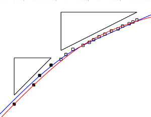
So, the Brooks & Corey (Reference Brooks and Corey1964) forms differ slightly from those of Lockington & Parlange (Reference Lockington and Parlange2004); technically either the permeability or hydraulic diffusivity, but not both simultaneously, can be matched. That said, the forms are effectively very similar as can be seen in a graphical comparison of the capillary pressure and permeability functions in figure 2. These comparisons capture the general features that (i) the capillary pressure builds from a unit reference pressure as the saturation drops away from one, and has a sharp increase at low saturation, and (ii) the permeability grows monotonically with saturation.

Figure 2. Panel (a) shows the dimensionless capillary pressure versus saturation curves for the Brooks–Corey model with $\lambda _{BC}=7.3$ and $S_r=0$ (black curve) and the Lockington–Parlange model with $\epsilon = \lambda _{BC}/(2 + 2 \lambda _{BC})$ and $\alpha = 14$ (red dashed curves and circles) and the Lockington–Parlange model with $\epsilon = \lambda _{BC}/(1 + 2\lambda _{BC})$ and $\alpha = 14$ (blue dotted curves and circles). Panel (b) shows the dimensionless permeability versus saturation curves for the Brooks–Corey model and Lockington–Parlange model for the same parameters and colour scheme as in (a). Note that the parameters for the red curves/circles were chosen to exactly match the Brooks–Corey and Lockington–Parlange permeability functions while the parameters for the blue curves/circles were chosen to match exponents of the Brooks–Corey and Lockington–Parlange hydraulic diffusivity functions. The key observation is that the Brooks–Corey functions match very closely with those employed in the Lockington–Parlange model.

Several other features of the Lockington–Parlange model are worth noting here. The early-time asymptotic behaviour of the Lockington–Parlange model in (3.1) and (3.2) corresponds to $Q_0 \gg 1$. We find that

(3.12)$$\begin{gather} Z_f = \left( 1 + \frac{1}{A} \right) \frac{1}{Q_0} - \left( 1 + \frac{1}{2A} \right) \frac{1}{Q_0^2} + O(Q_0^{{-}3}), \end{gather}$$

(3.13)$$\begin{gather}T = \frac{1}{2} \left( 1+\frac{1}{ A \sqrt{1 + 3\epsilon} } \right) \frac{1}{Q_0^2} + {O }(Q_0^{{-}3}). \end{gather}$$

This indicates that the early-time relationship between $Z_f$ and $T$ is

(3.14)\begin{equation} Z_f \sim \left( 1 + \frac{1}{A} \right) \sqrt{\frac{2 A \sqrt{1 + 3\epsilon} \; T }{1+ A \sqrt{1 + 3\epsilon} } } . \end{equation}

As noted by Lockington & Parlange (Reference Lockington and Parlange2004), with $A \rightarrow \infty$ the Washburn limit is recovered. However, outside of this limit ($1/A \neq 0$) both $A$ and $\epsilon$ influence the early-time dynamics and in general the details of the early-time Lockington & Parlange (Reference Lockington and Parlange2004) solution differ from those of the Washburn solution, although both follow the square-root in time scaling. The long-time asymptotic behaviour of the Lockington–Parlange model in (3.1) and (3.2) corresponds to $Q_0 \ll 1$. These two expressions can be expanded in this limit to reveal that

(3.15)$$\begin{gather} Z_f = \frac{1}{A} \ln \left( \frac{1}{Q_0} \right) + 1 + O(Q_0), \end{gather}$$

(3.16)$$\begin{gather}T = \frac{1}{A \sqrt{1 + 3\epsilon}} \frac{1}{Q_0} + \left(1 - \frac{1}{A \sqrt{1 + 3\epsilon}} \right) \ln \left( \frac{1}{Q_0} \right) - 1 + O(Q_0). \end{gather}$$

With $A \rightarrow \infty$ these give the expected Washburn limit $Z_f \rightarrow 1$. For finite $A$, these expressions show that $Z_{f}$ grows logarithmically in the long-time limit.

Our goals for revisiting the Lockington–Parlange model are three-fold. First, the Lockington–Parlange model is a relatively simple model involving closed form expressions and as such serves as a useful predictive tool and comparison for our free-boundary model. Second, to our knowledge, no quantitative comparison of the Lockington–Parlange model has been made to experimental data to the point where one can identify appropriate parameters $A$ and $\epsilon$ (Lockington & Parlange (Reference Lockington and Parlange2004) did demonstrate in their paper that their model recovers qualitatively the features of the Lago & Araujo (Reference Lago and Araujo2001) experiments). Third, with reasonable comparison with both classical and anomalous dynamics in hand, solutions to the Lockington–Parlange model (as well as our model solutions) will be used to reveal detailed information about permeability dynamics. In particular, we shall directly explore the recently proposed permeability versus capillary-rise dynamic scaling proposed by Kim et al. (Reference Kim, Ha and Kim2017) and Ha & Kim (Reference Ha and Kim2020).

4. Comparison with experimental data

Lago & Araujo (Reference Lago and Araujo2001) and Delker et al. (Reference Delker, Pengra and Wong1996) report capillary rise of water in a vertical column of glass beads connected to a reservoir of fluid. We obtained the Lago & Araujo (Reference Lago and Araujo2001) capillary rise versus time experimental data from their figure 10(a) using MATLAB's grabit.m software. We collected points from each of the curves corresponding to $150$–$180\ \mathrm {\mu }{\rm m}$, $180$–$212\ \mathrm {\mu }{\rm m}$, $212$–$250\ \mathrm {\mu }{\rm m}$ and $250$–$300\ \mathrm {\mu }{\rm m}$ glass bead sizes, and for simplicity refer to these below in tables and graphs by labels $150\ \mathrm {\mu }{\rm m}$, $180\ \mathrm {\mu }{\rm m}$, $212\ \mathrm {\mu }{\rm m}$ and $250\ \mathrm {\mu }{\rm m}$, respectively. These represent time and height data denoted by $(t_{exp}^i,h_{exp}^i)$ for $i=1, \ldots, N_{total}$ where $N_{total}$ is the number of data points. We used a similar procedure to obtain the Delker et al. (Reference Delker, Pengra and Wong1996) capillary-rise data from their figure 2(a). Four data sets were obtained corresponding to their experiments for $180\ \mathrm{\mu }{\rm m}$, $253\ \mathrm {\mu }{\rm m}$, $359\ \mathrm {\mu }{\rm m}$ and $510\ \mathrm {\mu }{\rm m}$ bead diameters.

A technical but important detail about the Lago & Araujo (Reference Lago and Araujo2001) capillary-rise data is that at their time zero the fluid height is at the reservoir height, $z_R$ (see figure 1). Figure 2(a) of Delker et al. (Reference Delker, Pengra and Wong1996) shows capillary-rise height relative to $z=0$ with their starting time also corresponding to when the capillary-rise height is equal to $z_R$. To put the Delker et al. (Reference Delker, Pengra and Wong1996) data in the form of the Lago & Araujo (Reference Lago and Araujo2001) data, we shift the Delker et al. (Reference Delker, Pengra and Wong1996) height values by $z_R$ (in their notation this is $Z - z_R$). In contrast, our model (and that of the Lockington–Parlange model) has time $t=0$ corresponding to $h_{\ell } = 0$. Therefore, in order to compare our predictions with the experiments we plot $h_{\ell }(t) - z_R$ versus $t - t_R$ where $t_R$ is defined to be the time for which $h_{\ell }(t_R) = z_R$ (in the Lockington–Parlange model we similarly plot $z_f - z_R$ versus $t - t_R$). Thus, ‘early time’ in the experimental plots means $t - t_R \ll 1$ in our model notation. A consequence of this is that the plotted capillary-rise height $h_{\ell }(t) - z_R$ for early time is linear in $t- t_R$ whenever $z_R \neq 0$. Further details of this are explained below.

In addition to comparing the Lago & Araujo (Reference Lago and Araujo2001) and Delker et al. (Reference Delker, Pengra and Wong1996) data with our model and the Lockington–Parlange model we briefly revisit the Washburn model. From a parameter estimation point of view, the Washburn model, as outlined below, involves three-dimensional parameters $h_e$, $z_R$ and $v_g$. For the Lockington–Parlange model five parameters appear: the dimensional ones $h_e$, $z_R$ and $v_g$, along with the dimensionless parameters $A$ and $\epsilon$. For our free-boundary model there are five as well: $h_e$, $z_R$, $v_g$ and the two dimensionless parameters $S_1$ and $\lambda _{BC}$.

Our optimization procedure to identify parameters involves minimizing the mean square error of capillary-rise height at the available experimental time points. We have used absolute errors in all cases described here but note that relative errors and/or other weighting schemes could be implemented. Our numerical scheme uses MATLAB's fmincon to search the parameter space. We have explored both interior-point and sqp algorithms with a variety of initial guesses to help find the best solution within our search space. In each case we limit our parameter search space with upper and lower bounds on each parameter. Some of these bounds are based on previous estimates in Lago & Araujo (Reference Lago and Araujo2001) and/or Delker et al. (Reference Delker, Pengra and Wong1996), especially with respect to the parameters $h_e$, $v_g$ and $z_R$, and are explained in detail below. The models of primary interest – the Lockington–Parlange model and our free-boundary model – have five-dimensional search spaces and even with bounds on these parameters we cannot guarantee that our reported solutions are global optimizers. Rather, we seek parameter values that are consistent with prior information and also reasonably fit the capillary-rise versus time data. With reasonable fits to the capillary-rise dynamics in both early- and long-time regimes we then further explore our model predictions on capillary pressure and permeability dynamics, which are not as easily accessible experimentally, and help shed further light on the capillary-rise phenomena.

The first step of our parameter estimation procedure involves fitting a linear function $t - t_R = P_1 (h_{\ell } - z_R)$ to early time data of Lago & Araujo (Reference Lago and Araujo2001) and Delker et al. (Reference Delker, Pengra and Wong1996) where $P_1$ has units of seconds per centimetre. That this early-time data has this linear structure, rather than the celebrated $t^{1/2}$ scaling, relates to the space and time shift of the data, and will be demonstrated in the context of the models below. We report numerical values of $P_1$ in table 1 for each Lago & Araujo (Reference Lago and Araujo2001) and Delker et al. (Reference Delker, Pengra and Wong1996) data set and note that these values of $P_1$ are independent of the theoretical model (Washburn, Lockington–Parlange, $\ldots$). The value of $N$ indicates the number of data points used in the fits. We see that the value of $P_1$ is relatively insensitive at small values of $N$ but necessarily drifts to larger values as more time points are included and the dynamics depart from the early-time behaviour. We have listed estimates and standard deviations in each case on the lines marked by $*$ in table 1.

Table 1. Fitted leading coefficient, $P_1$, from the model independent relation $t - t_R = P_1 (h_{\ell } - z_R)$ using capillary-rise data of Lago & Araujo (Reference Lago and Araujo2001) and Delker et al. (Reference Delker, Pengra and Wong1996). Here $N$ is the number of early time points used in the fit. Note that the case for Delker et al. (Reference Delker, Pengra and Wong1996) 510 $\mathrm {\mu }$m beads only has six data points that appear to fall in the early-time regime. The mean and standard deviation for $P_1$ using the first four points ($N=6,7,8,9$ for Lago & Araujo (Reference Lago and Araujo2001) and $N=3,4,5,6$ for Delker et al. (Reference Delker, Pengra and Wong1996)) are listed on the lines marked by the $*$.

As shown below, in the Washburn model we can identify $P_1 = P_1^{Wash} = z_R/(v_g h_e)$ which fixes a relationship between the three parameters $h_e$, $v_g$ and $z_R$. In the Lockington–Parlange model $P_1 = P_1^{LP}$ where $P_1^{LP}$ depends on $z_R$, $h_e$ and $v_g$ as well as on $A$ and $\epsilon$. Similarly, for our free-boundary model $P_1 = P_1^{SA}$ where $P_1^{SA}$ depends on $z_R$, $h_e$ and $v_g$ as well as on $S_1$ and $\lambda _{BC}$. With these relationships, we choose to replace our search variable $v_g$ with the search variable $P_1$. The reported mean plus-or-minus the standard deviation for each data set in table 1 then provides upper and lower bounds for the $P_1$ search space.

Before reporting further details on the parameter estimation for the Washburn, Lockington–Parlange and free-boundary models, we give an example solution from our free-boundary model in figure 3 with dimensional heights of the wetting front (solid curve), the saturated/unsaturated front (dashed curve – , i.e. Washburn solution) and the early time linear relationship (dashed–dotted curve), along with the Lago & Araujo (Reference Lago and Araujo2001) $150\ \mathrm {\mu }{\rm m}$ data (open circles). This plot shows the relationship of the two interface positions, $h_{\ell }^S$ and $h_{\ell }$, along with the early-time linearization. The boundary $h_{\ell }^S$ (which is equivalent to the Washburn model) reaches an equilibrium height while $h_{\ell }$ continues to increase in good approximation to the experimental observations.

Figure 3. An example of our free-boundary model predictions: Lago & Araujo (Reference Lago and Araujo2001) data for $150\ \mathrm {\mu }{\rm m}$ spheres (open circles); the linear approximation $h_{\ell } - z_R \sim (1/P_1^{SA}) (t - t_R)$ (dash–dotted line); the prediction $h_{\ell } - z_R$ versus $t- t_R$ (solid curve); $h_{\ell }^S - h_{\ell }^S(t_R)$ versus $t-t_R$ (dotted line). Note that $h_{\ell }^S$ is equivalent to the Washburn solution.

4.1. Washburn model predictions

The dimensional form of the classical Washburn model (e.g. using the Lockington–Parlange equations (3.1) and (3.2) with $A \rightarrow \infty$), is

(4.1)\begin{equation} t_{Wash} = \frac{h_e + z_R}{v_g} \ln \left( \frac{z_R + h_e}{z_R + h_e - z_f} \right) - \frac{z_f}{v_g}, \end{equation}

where $t_{Wash}$ is time and $z_f$ is the capillary-rise height relative to fixed position $z=0$. This form has $z_f=0$ when $t_{Wash}=0$ and $z_f \rightarrow z_R + h_e$ as $t_{Wash} \rightarrow \infty$. It is worth noting that for early time $z_f$ and $t_{Wash}$ have the classical relationship

(4.2)\begin{equation} z_f \sim \sqrt{2 v_g (z_R + h_e) t_{Wash}} \sim t_{Wash}^{1/2}. \end{equation}

As previously noted, in order to compare equation (4.1) with the experiments of Lago & Araujo (Reference Lago and Araujo2001) we need a time- and space-shifted version. The capillary-rise height and time variables used in Lago & Araujo (Reference Lago and Araujo2001) (see their figure 10a) are the shifted versions $z_f - z_R$ and $t_{Wash} - t_R$, where $t_R$ is defined as the time for which $z_f = z_R$. That is,

(4.3)\begin{equation} t_R= \frac{h_e + z_R}{v_g} \ln \left( \frac{z_R + h_e}{h_e} \right) - \frac{z_R}{v_g}, \end{equation}

and

(4.4)\begin{equation} t_{Wash} - t_R = \frac{h_e + z_R}{v_g} \ln \left( \frac{h_e}{h_e - (z_f - z_R)} \right) - \frac{z_f - z_R}{v_g}. \end{equation}

In this view the early-time dynamics are characterized by the relationship

(4.5)\begin{equation} t_{Wash} - t_R = \frac{z_R}{v_g h_e} (z_f - z_R) + \frac{z_R + h_e}{2 v_g h_e^2} (z_f - z_R)^2 + \cdots. \end{equation}

That is, unless the reservoir height $z_R=0$, the capillary-rise height in the Lago & Araujo (Reference Lago and Araujo2001) interpretation scales linearly with early times. The dynamics are still classical in the sense that they are characterized by the Washburn equation but the capillary-rise height does not display the commonly referred to $t^{1/2}$ power law (e.g. see their figure 10a and/or our figure 4). Here we define $P_1^{Wash} = z_R/(v_g h_e)$.

Figure 4. Panel (a) shows capillary-rise height versus time predictions with the Lockington–Parlange model using the parameter values listed in table 3 and the Lago & Araujo (Reference Lago and Araujo2001) data. Panel (b) shows capillary-rise height versus time predictions with the Lockington–Parlange model using the parameter values listed in table 3 and the Delker et al. (Reference Delker, Pengra and Wong1996) data. The triangles indicate power-law slopes of $1$ (left-hand triangle), $1/4$ (upper right-hand triangle) and $1/20$ (lower right-hand triangle).

We note that if given capillary-rise data in the form $(t_{Wash}, z_f)$ the model in (4.1) would allow at most the determination of two independent parameters, $v_g$ and the combination $h_e + z_R$ (that is, one cannot get $z_R$ and $h_e$ individually without additional information). On the other hand, given sufficient data in the form $(t_{Wash}-t_R, z_f- z_R)$ the model in (4.4) does appear to allow the determination of three independent parameters, $v_g$, $h_e$ and $z_R$.

We comment here on upper and lower bounds for the parameters $P_1$, $z_R$ and $h_e$. First, as already mentioned, the search space for the parameter $P_1$ was limited for each data set by the range listed in table 1. Second, bounds for the parameter $z_R$ were identified in two different ways for the Lago & Araujo (Reference Lago and Araujo2001) and Delker et al. (Reference Delker, Pengra and Wong1996) data sets. Delker et al. (Reference Delker, Pengra and Wong1996) reported in their experiments that $z_R$ was approximately $4$ cm and so for these cases we have simply allowed a small departure ($\pm 0.1$ cm) from this value. In most cases (with the Washburn model, as well as the Lockington–Parlange model, and our free-boundary model) we found that the upper bound $z_R = 4.1$ cm was an active constraint. In general, while extending the range of $z_R$ could allow small numerical reductions in our objective function there were not significant graphical improvements that would seem to justify allowing further departures from $4$ cm estimate reported by Delker et al. (Reference Delker, Pengra and Wong1996). Lago & Araujo (Reference Lago and Araujo2001) did not report values for their $z_R$. However, they did report ranges for $h_e$ and for $v_g$ (see their figure 11a,b) and since they also report fits based on the Washburn model we identified bounds for their $z_R$ using the Washburn relation $P_1 = z_R/(h_e v_g)$ and the $P_1$ values reported in table 1. The $z_R$ values we found for the Lago & Araujo (Reference Lago and Araujo2001) data were in all cases within these bounds with no active constraints. Third, for the parameter $h_e$ we chose generous bounds that included the full range of $h_e$ reported for the Lago & Araujo (Reference Lago and Araujo2001) data sets (see their figure 11a). We expect $h_e \sim \sigma /(\rho g D_b)$ (i.e. Jurin height) where $\sigma$ is surface tension, $\rho$ is fluid density, $g$ is gravity and $D_b$ is the bead diameter. Using $\sigma = 72\,{\rm mN}\,{\rm m}^{-1}$, $\rho = 10^3\,{\rm kg}\,{\rm m}^{-3}$ and $g=9.8\,{\rm m}\,{\rm s}^{-2}$ gives $h_e \sim [4.9, 4.1, 3.5, 2.9]\,{\rm cm}$ for the Lago & Araujo (Reference Lago and Araujo2001) data and $h_e \sim [4.1, 2.9, 2.0, 1.4]\,{\rm cm}$ for the Delker et al. (Reference Delker, Pengra and Wong1996) data.

The bounds for $P_1$, $z_R$ and $h_e$ are shown in table 2; these are also later used for the Lockington–Parlange model and our free-boundary model. Our Washburn model estimates for $h_e$, $z_R$, $P_1$ and $v_g$ are listed in table 2. It is important to note that for the Washburn model one must also decide how much of the capillary rise data to fit (i.e. make a choice for $N$) as the long-time behaviour of the data is not described by the Washburn model. Recall that the Washburn model predictions have the form of the dotted curve shown in figure 3. Making $N$ too large and trying to fit the capillary-rise data in the anomalous regime will artificially drive up the value of $h_e$. Making $N$ too small and not including enough information about the transition away from the early-time dynamics will not allow identification of $h_e$ and $z_R$. That said, the parameter values in table 2 are generally consistent with various earlier estimates reported by Lago & Araujo (Reference Lago and Araujo2001) and Delker et al. (Reference Delker, Pengra and Wong1996). Our primary purpose in generating estimates for these parameters from the Washburn model is to have a point of reference when we obtain estimates for these same parameter values for the Lockington–Parlange model and our free-boundary model, both of which are better suited to characterize the long-time dynamics.

Table 2. Fitted Washburn model parameters $h_e$ and $z_R$ for capillary-rise data of Lago & Araujo (Reference Lago and Araujo2001) and Delker et al. (Reference Delker, Pengra and Wong1996) using values of $P_1$ in the range specified in table 1, and the resultant value $v_g = z_R/(P_1 h_e)$. The range indicated by the brackets are those imposed as constraints during the optimization procedure. The number of points, $N$, used for the fits is listed in parentheses and has been chosen in a range where the estimates for $h_e$ and $z_R$ are relatively insensitive to $N$.

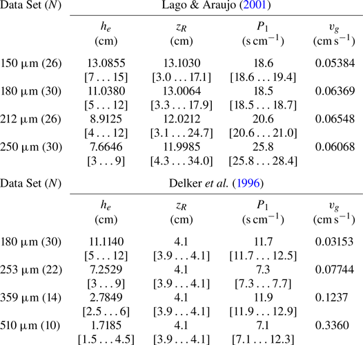
4.2. Lockington–Parlange model predictions

The Lockington–Parlange model with dimensionless capillary-rise height $Z_f$ and time $T$ is given by (3.1) and (3.2). We note that $Z_f$ reaches the dimensionless reservoir height, $Z_R = z_R/(z_R + h_e)$, at a time $T_R$ for which $Q_0=Q_R$. That is,

(4.6)$$\begin{gather} Z_R = \frac{1}{A} \ln \left( \frac{Q_R + 1}{Q_R} \right) + \frac{1}{Q_R + 1}, \end{gather}$$

(4.7)$$\begin{gather}T_R = \ln \left( \frac{Q_R + 1}{Q_R} \right) - \frac{1}{Q_R + 1} + \frac{1}{A \sqrt{1 + 3 \epsilon} } \left[ \frac{1}{Q_R} - \ln \left( \frac{Q_R + 1}{Q_R} \right) \right], \end{gather}$$

where (4.6) determines the value of $Q_R$ for a given reservoir height $Z_R$ and the corresponding time is given by (4.7).

The early time, $0 \le T-T_R \ll 1$, form of $Z_f - Z_R$ is

(4.8)\begin{equation} Z_f - Z_R = Q_R \frac{1 + \dfrac{1}{A} \left( 1 + \dfrac{1}{Q_R} \right)}{1 + \dfrac{1}{A \sqrt{1 + 3 \epsilon} } \left( 1 + \dfrac{1}{Q_R} \right)} \left( T-T_R \right) + O\left( T-T_R \right)^2. \end{equation}

The corresponding dimensional quantities are $z_f - z_R = (Z_f - Z_R) (z_R + h_e)$ and $t-t_R = (T - T_R) (z_R + h_e)/v_g$. Then, the dimensional leading-term in (4.8) is

(4.9)\begin{equation} z_f - z_R \sim v_g \left[ Q_R \frac{1 + \dfrac{1}{A} \left( 1 + \dfrac{1}{Q_R} \right)}{1 + \dfrac{1}{A \sqrt{1 + 3 \epsilon} } \left( 1 + \dfrac{1}{Q_R} \right)}\right] \left( t-t_R \right). \end{equation}

That is, the early-time data is fit by taking $P_1^{LP} = P_1$ where

(4.10)\begin{equation} P_1^{LP} = \frac{1}{v_g Q_R} \frac{1 + \dfrac{1}{A \sqrt{1 + 3 \epsilon} } \left( 1 + \dfrac{1}{Q_R} \right)}{1 + \dfrac{1}{A} \left( 1 + \dfrac{1}{Q_R} \right)}, \end{equation}

which is a non-trivial function of the ratio $h_e/z_R$ (through $Z_R$ and $Q_R$), $A$ and $\epsilon$. When $A \rightarrow \infty$, we find that $Q_R \rightarrow h_e/z_R$ and $P_1^{LP} \rightarrow z_R/(v_g h_e)$ as in the leading behaviour of the Washburn model analogue (4.5).

We fit the full Lockington–Parlange model $z_f - z_R$ versus $t - t_R$ for all times available in the Lago & Araujo (Reference Lago and Araujo2001) and Delker et al. (Reference Delker, Pengra and Wong1996) data sets. Our search space is over the parameters $h_e$, $z_R$, $A$, $\epsilon$ and $P_1$ with ranges as listed in brackets in table 3. The bounds on $P_1$, $z_R$, and $h_e$ are the same as those already identified in the discussion of the Washburn model. The search space for the parameter $A$ was effectively left unconstrained although for technical reasons we typically set bounds $[0 \ldots 100]$. We used $[0 \ldots 1]$ as the search space for the parameter $\epsilon$ with it in mind that the Lockington–Parlange model assumed $\epsilon \ll 1$. The value of $v_g$ was obtained through the condition $P_1^{LP} = P_1$.

Table 3. Lockington–Parlange model parameters $A$, $\epsilon$, $h_e$ and $z_R$ for capillary-rise data of Lago & Araujo (Reference Lago and Araujo2001) and Delker et al. (Reference Delker, Pengra and Wong1996) using $P_1$ in the range indicated in table 1 with the resultant value $v_g$ obtained from the relationship (4.10). The range indicated in the $A$, $\epsilon$, $h_e$, $z_R$ and $P_1$ columns correspond to the allowed search space.

The parameter value estimates for the Lockington–Parlange model are listed in table 3. In some of these cases the constraints on the parameter are active, which generally indicates that one can find solutions with numerically smaller objective function values if these bounds were extended. Two examples of note are the solutions for the Delker et al. (Reference Delker, Pengra and Wong1996) 359 $\mathrm {\mu }$m and 510 $\mathrm {\mu }$m cases which have active lower bounds on $h_e$. In these two cases the Lockington–Parlange model predictions appear to fit the data only moderately well (see figure 4). These graphical comparisons could be improved slightly by allowing significantly smaller values of $h_e$. For example, for the 359 $\mathrm {\mu }$m Delker et al. (Reference Delker, Pengra and Wong1996) data the parameter set [$A=9.32$, $\epsilon = 0.0036$, $h_e = 0.39$ cm, $z_R = 4.1$ cm and $P_1 = 11.9$ s cm$^{-1}$] has $F=3.6056$ which is a graphical and numerical improvement over the case listed in table 3 and shown in figure 4. However, the value $h_e = 0.39$ cm appears to be inconsistent (approximately a factor of 10 too small) with what would be expected using the Jurin scaling and the estimate for $h_e$ for the 180 $\mathrm {\mu }$m bead diameter; that is, $\approx 6.7/2 = 3.35$ cm.

It appears from figure 4 that for the majority of these cases, except for largest two bead diameter results of Delker et al. (Reference Delker, Pengra and Wong1996), the Lockington–Parlange model is able to capture essential features of the dynamics from the early-time, classical dynamics all the way through the long-time, anomalous dynamics, evolution. Lago & Araujo (Reference Lago and Araujo2001) have already reported an estimated range of scaling exponents for their long-time power laws between ${1/20}$ and ${1/4}$. For comparison purposes we have indicated these particular scaling estimates on the graph. For both the Lago & Araujo (Reference Lago and Araujo2001) data and the Delker et al. (Reference Delker, Pengra and Wong1996) data the anomalous scaling in the long-time dynamics seems to lie somewhere in between these values. The speed and ease of use of the Lockington–Parlange model are advantages over the free-boundary model discussed next, although we shall see that the ability to characterize the Delker et al. (Reference Delker, Pengra and Wong1996) large bead data, appears to be an advantage of the free-boundary model.

4.3. Free-boundary model with Brooks–Corey function predictions

Here we compare our model with Brooks–Corey functions for capillary pressure and permeability to the capillary-rise experiments of Lago & Araujo (Reference Lago and Araujo2001) and Delker et al. (Reference Delker, Pengra and Wong1996) These solutions were obtained computationally as follows. An initial condition for the partial differential equation for saturation on $\bar {h}_{\ell }^S < \bar {z} < \bar {h}_{\ell }$ was obtained using the similarity solution. In particular, the similarity solution starts with initial conditions $\bar {h}_{\ell }^S(\bar {t}=0)=\bar {h}_{\ell }(\bar {t}=0)=0$ and is used to advance forward in time to a small but non-zero value $\bar {t}^*$ where $\bar {h}_{\ell }^S(\bar {t}^*)$ and $\bar {h}_{\ell }(\bar {t}^*)$ are non-zero and a saturation profile $S(\bar {z},\bar {t}^*)$ from the similarity solution is also obtained. An example saturation curve from the similarity solution used to start the numerical simulations is shown in figure 5(a). Note that this example has dimensional time $t^* = 0.0081$ s and has $h_{\ell }(t^*) > h_{\ell }^S(t^*) >0$. The partial differential equation was discretized in space over the partially saturated region with $N_{pde}+1$ evenly spaced points. We used a range of values of $N_{pde}$ up to $N_{pde}=2048$. Several example solutions for $S(z,t)$ are shown in figure 5(b). We observe that the saturation decreases monotonically at higher positions in the partially saturated media with the variation more pronounced at later times. This example corresponds to a base-case set of parameters from which we explore the solution dependence on the parameters $S_1$ and $\lambda _{BC}$ further below. Parameter estimation for this model was performed in a similar manner to that done for the Washburn model and the Lockington–Parlange model. Details specific to this model involving the interpretation of parameter $P_1$ and the search space used for parameters $S_1$ and $\lambda _{BC}$ are outlined below.

Figure 5. Panel (a) shows the similarity solution $S(z,t)$ plotted against $z- z_R$ at the time value $t= t^* = 0.0081$ s. This function $S(z,t^*)$, along with the values $h_{\ell }(t^*)$ and $h_{\ell }^S(t^*)$, from the similarity solution are used as the initial conditions (at $t=t^*$) for the numerical integration of the free-boundary problem defined in (2.25), (2.26) and (2.27). Note that the red ‘o’ in (a) at $S=1$ corresponds to $h_{\ell }^S(t^*) - z_R$ (i.e. $z=h_{\ell }^S(t^*)$) while the red ‘x’ in this same plot near $S=0$ corresponds to $h_{\ell }(t^*) - z_R$ (i.e. $z=h_{\ell }(t^*)$). Panel (b) shows the full numerical solution $S(z,t)$ – with initial condition indicated in panel (a) – at various times plotted against the shifted coordinate $z - z_R$. In this plot, the ‘o’ marks at $S=1$ correspond to $h_{\ell }^S(t) - z_R$ at the indicated times while the ‘x’ marks near $S=0$ correspond to $h_{\ell }(t) - z_R$ at those times. The parameter values used for this example are $\lambda _{BC}=3.32$, $S_1=0.01$, $h_e = 9.8$ cm, $P_1 = 18.6$ s cm$^{-1}$ and $z_R = 7.5$ cm, which correspond to the values used for the solid curves in figure 6(a,b).

As a first step in the parameter identification for this free-boundary model we identify a parameter that we can associate with the experimentally identified values of $P_1$ (see table 1) which characterize capillary rise dynamics near the time $t = t_R$ for which $h_{\ell } = z_R$. The local expansion of our dimensionless solution is

(4.11)\begin{equation} \bar{h}_{\ell} - \bar{z}_R \sim \left. \frac{{\rm d} \bar{h}_{\ell}}{{\rm d}\bar{t}} \right|_{\bar{t} = \bar{t}_R} ( \bar{t} - \bar{t}_R), \end{equation}

where from (2.26) we have that

(4.12)\begin{equation} {\mathcal{D}} \equiv \left. \frac{{\rm d} \bar{h}_{\ell}}{{\rm d}\bar{t}} \right|_{\bar{t} = \bar{t}_R} ={-} \frac{1}{\lambda_{BC}} S_1^{1 + 1/\lambda_{BC}} \left. \frac{\partial S}{\partial \bar{z}} \right|_{\bar{z} = \bar{h}_{\ell}(\bar{t}_R)} - \frac{1}{1-\bar{z}_R} S_1^{2 + 2/\lambda_{BC}}. \end{equation}

We do not have an analytical expression for the saturation derivative appearing here but it is computed as part of our solution. In dimensional form we have $t - t_R \sim P_1^{SA} (h_{\ell } - z_R)$ where

(4.13)\begin{equation} P_1^{SA} = \frac{h_e + z_R}{h_e v_g} \frac{1}{ {\mathcal{D}} }. \end{equation}

Before discussing additional details of our model comparison with the Lago & Araujo (Reference Lago and Araujo2001) and Delker et al. (Reference Delker, Pengra and Wong1996) data we explore how the two model parameters $S_1$ and $\lambda _{BC}$ influence the dynamics. Figure 6 shows capillary-rise height $h_{\ell }(t) - z_R$ versus $t-t_R$ as the two parameters $S_1$ and $\lambda _{BC}$ are individually varied. The long-time dynamics are sensitive to both of these parameters. Note that using the equilibrium expressions in (2.17) and (2.18) with the Brooks–Corey expression for capillary pressure in (2.23a,b) gives

(4.14)\begin{equation} h_{\ell}(t \rightarrow \infty) = z_R + h_e \left( \frac{1}{S_1} \right)^{{1}/{\lambda_{BC}}} . \end{equation}

This shows that $h_{\ell }(t \rightarrow \infty ) \rightarrow \infty$ as $S_1 \rightarrow 0$ while $S_1 = 1$ recovers the Washburn equilibrium. These trends can be observed in figure 6. The smaller $S_1$ leads to a higher capillary-rise height. All of our numerical simulations have used non-zero $S_1$ and so all of these predictions eventually reach an equilibrium height. In this particular example in figure 6 the data of Lago & Araujo (Reference Lago and Araujo2001) for the 150 $\mathrm {\mu }$m bead diameter are shown and their final experimental data point has a capillary-rise height of around $26$ cm. For sufficiently small $S_1$ the theoretical equilibrium height $h_{\ell }(t \rightarrow \infty )$ is well above this value. In general, the Lago & Araujo (Reference Lago and Araujo2001) data and the Delker et al. data provide capillary-rise data out to times around 24 hours. We are not aware of experimental data for these systems that could test the model predictions, such as the possibility of an eventual plateau in capillary-rise height, beyond these times.

Figure 6. Panel (a) shows four capillary-rise solutions as $S_1$ varies with $\lambda _{BC}=3.32$, $h_e = 9.8$ cm, $P_1 = 18.6$ s cm$^{-1}$ and $z_R = 7.5$ cm. Panel (b) shows four capillary-rise solutions as $\lambda _{BC}$ varies with $S_1 = 0.01$, $h_e = 9.8$ cm, $P_1 = 18.6$ s cm$^{-1}$ and $z_R = 7.5$ cm. For reference we have also included the Lago & Araujo (Reference Lago and Araujo2001) $150\ \mathrm {\mu }$m data.

Our best parameter estimates in comparison with the Lago & Araujo (Reference Lago and Araujo2001) and Delker et al. (Reference Delker, Pengra and Wong1996) data are listed in table 4 with the corresponding graphical results shown in figure 7. The search space in each case is indicated and for parameters $h_e$, $z_R$ and $P_1$ these bounds are the same as used previously for the Washburn and Lockington–Parlange models. The upper and lower bounds for the parameters $S_1$ and $\lambda _{BC}$ are also listed and were chosen to effectively keep these parameters unconstrained; none of these constraints are active. Again we do not guarantee that the reported solutions are globally optimal in the prescribed feasible set but in all of these cases the graphical comparison with the data is excellent, especially in the long-time, anomalous, regime.

Table 4. Parameter values for $S_1$, $\lambda _{BC}$, $h_e$ and $z_R$ for our free-boundary model with Brooks–Corey functions for capillary rise data of Lago & Araujo (Reference Lago and Araujo2001) and Delker et al. (Reference Delker, Pengra and Wong1996) using the values of $P_1$ indicated by the range given in table 1 with the resultant value $v_g$ obtained from the expression (4.13). The range indicated in the $S_1$, $\lambda _{BC}$, $h_e$, $z_R$ and $P_1$ columns correspond to ranges allowed for these parameters in our parameter search.

Figure 7. Panel (a) shows capillary-rise height versus time predictions with our model using the parameter values listed in table 4 and the Lago & Araujo (Reference Lago and Araujo2001) data. Panel (b) shows capillary-rise height versus time predictions with our model using the parameter values listed in table 4 and the Delker et al. (Reference Delker, Pengra and Wong1996) data.

The solutions reported in tables 3 and 4 along with the graphical counterparts in figures 4 and 7 show that both the Lockington–Parlange and free-boundary models can capture many features of the capillary-rise dynamics for both early- and long-time regimes. We note that there is some variation across models in terms of the predicted values of $h_e$, $v_g$ and $z_R$. As we have shown, the early-time fit establishes a value of the parameter $P_1$ for a given data set, but depending on the model (Washburn, Lockington–Parlange or the free-boundary formulation) the relationships that $h_e$, $v_g$ and $z_R$ have with the parameter $P_1$ differ. That is, other parameters ($A$ and $\epsilon$ for Lockington–Parlange and $\lambda _{BC}$ and $S_1$ for the free-boundary model) also are involved in the corresponding expressions for $P_1$ and, consequently, the fit values of $h_e$, $v_g$ and $z_R$ (if not measured independently in an experiment) are at least slightly model dependent. We have chosen to allow a range for each of these parameters, as noted in the tables. The Lockington–Parlange model perhaps does slightly better numerically for the Lago & Araujo (Reference Lago and Araujo2001) data while the free-boundary model appears to do better for the Delker et al. (Reference Delker, Pengra and Wong1996) data. We note that the two cases corresponding to the largest bead diameter for the Delker et al. (Reference Delker, Pengra and Wong1996) data show that the capillary-rise dynamics has positive concavity. The prediction of the free-boundary model also has this characteristic for these two cases. The 359 $\mathrm {\mu }$m and $510\ \mathrm {\mu }{\rm m}$ predictions suggest that the larger bead diameter prediction reaches a larger capillary-rise height (compare $S_1=0.0007$ for the 359 $\mathrm {\mu }$m case with $S_1 = 0.001$ for the 510 $\mathrm {\mu }$m case) for times beyond where the experimental data is available. We presume this particular observation may change were further experimental data available for these cases beyond the reported final time.

5. Permeability and capillary pressure measures and their dynamic scaling

In the introduction we reviewed scaling laws initially developed for capillary-rise phenomena in partially saturated porous media by Kim et al. (Reference Kim, Ha and Kim2017) and Ha & Kim (Reference Ha and Kim2020). Their arguments suggested that at early times both the capillary pressure and the permeability scale independently of capillary-rise height. At later times there is a capillarity–gravity balance in which capillary pressure scales linearly with height and the permeability scales inversely proportional to capillary-rise height squared. We explore these ideas further here.

In both of the capillary-rise models presented in this work – the Lockington–Parlange model and our free-boundary model with Brooks–Corey functions – the capillary pressure and permeability are defined throughout the partially saturated region (as well as the completely saturated region) and therefore have both spatial and temporal variation. The question then arises that if, for example, the scaling law $k \sim 1/h^2$ holds, where specifically in the partially saturated region does it hold? Throughout the entire partially saturated region, or in some specific region? By examining the computed permeability function through the identification of representative permeability measures over different regions in the partially saturated media we can address this question. For our free-boundary model we discuss analogue capillary pressure measures as well.

We begin with the Lockington–Parlange model where integrals of the permeability can be expressed in simple terms. Since those results were not part of the original work presented in Lockington & Parlange (Reference Lockington and Parlange2004) we provide details in Appendix B. The four permeability measures we use here correspond to mean permeabilities taken from the bottom quarter to the top quarter of the partially saturated region. In particular, we define

(5.1)$$\begin{gather} \bar{K}^{eff}_{I}(t) ={-}\frac{4}{\Delta Z} \int_{0}^{{-}u_1^*} \frac{\exp [A (1+\epsilon) u]}{1+Q_0 \exp [{-}A u] } \,{\rm d}u, \end{gather}$$

(5.2)$$\begin{gather}\bar{K}^{eff}_{II}(t) ={-}\frac{4}{\Delta Z} \int_{{-}u_1^*}^{{-}u_2^*} \frac{\exp [A (1+\epsilon) u]}{1+Q_0 \exp [{-}A u] } \,{\rm d}u, \end{gather}$$

(5.3)$$\begin{gather}\bar{K}^{eff}_{III}(t) ={-}\frac{4}{\Delta Z} \int_{{-}u_2^*}^{{-}u_3^*} \frac{\exp [A (1+\epsilon) u]}{1+Q_0 \exp [{-}A u] } \,{\rm d}u, \end{gather}$$

(5.4)$$\begin{gather}\bar{K}^{eff}_{IV}(t) ={-}\frac{4}{\Delta Z} \int_{{-}u_3^*}^{-\infty} \frac{\exp [A (1+\epsilon) u]}{1+Q_0 \exp [{-}A u] } \,{\rm d}u, \end{gather}$$

where $\Delta Z = Z_f - Z_e$, $Z_e = 1/(Q_0 + 1)$ and $Z_f$ and $Q_0$ are as in (3.1) and (3.2). For $i= 1,2,3$ we have

(5.5)\begin{equation} {-}u_i = \frac{1}{A} \ln \left[{-}Q_0 + (1+Q_0) {\rm e}^{\omega_i} \right],\quad \omega_i ={-} \frac{i}{4} A \Delta Z, \end{equation}

which define the integration limits. We also define an overall effective permeability for the whole partially saturated region which has $\bar {K}^{eff}(t) = ( \bar {K}^{eff}_{I}(t) + \bar {K}^{eff}_{II}(t) + \bar {K}^{eff}_{III}(t) + \bar {K}^{eff}_{IV}(t))/4$. We discuss these results below in the context of similar permeability measures from the free-boundary model.

For the free-boundary model we use the same choices for effective permeability. In this approach, the saturation variable is computed numerically and the corresponding permeability is defined by the Brooks–Corey model in (2.23a,b). In particular, dividing the partially saturated porous material into four quarters leads to

(5.6)$$\begin{gather} \bar{K}^{eff}_{I}(t) = \frac{4}{\bar{h}_{\ell}- \bar{h}_{\ell}^S} \int_{\bar{h}_{\ell}^S}^{\bar{h}_{\ell}^S + (\bar{h}_{\ell}- \bar{h}_{\ell}^S)/4} \bar{k}_{r\ell} (S(z,t)) \,{\rm d}z, \end{gather}$$

(5.7)$$\begin{gather}\bar{K}^{eff}_{II}(t) = \frac{4}{\bar{h}_{\ell}- \bar{h}_{\ell}^S} \int_{\bar{h}_{\ell}^S + (\bar{h}_{\ell}- \bar{h}_{\ell}^S)/4}^{\bar{h}_{\ell}^S + (\bar{h}_{\ell}- \bar{h}_{\ell}^S)/2} \bar{k}_{r\ell} (S(z,t)) \,{\rm d}z, \end{gather}$$

(5.8)$$\begin{gather}\bar{K}^{eff}_{III}(t) = \frac{4}{\bar{h}_{\ell}- \bar{h}_{\ell}^S} \int_{\bar{h}_{\ell}^S + (\bar{h}_{\ell}- \bar{h}_{\ell}^S)/2}^{\bar{h}_{\ell}^S + 3(\bar{h}_{\ell}- \bar{h}_{\ell}^S)/4} \bar{k}_{r\ell} (S(z,t)) \,{\rm d}z, \end{gather}$$

(5.9)$$\begin{gather}\bar{K}^{eff}_{IV}(t) = \frac{4}{\bar{h}_{\ell}- \bar{h}_{\ell}^S} \int_{\bar{h}_{\ell}^S + 3(\bar{h}_{\ell}- \bar{h}_{\ell}^S)/4}^{\bar{h}_{\ell}} \bar{k}_{r\ell} (S(z,t)) \,{\rm d}z. \end{gather}$$

We also examine $\bar {K}^{eff}(t) = ( \bar {K}^{eff}_{I}(t) + \bar {K}^{eff}_{II}(t) + \bar {K}^{eff}_{III}(t) + \bar {K}^{eff}_{IV}(t))/4$ which is the mean over the whole partially saturated region. Analogue measures for capillary pressure with $\bar {k}_{r\ell }$ replaced by $\bar {p}_c$ will also later be discussed.

Figure 8 shows two plots of effective permeability versus capillary-rise height. Figure 8(a) corresponds to the Lockington–Parlange model for the example based on the Lago & Araujo (Reference Lago and Araujo2001) 150 $\mathrm {\mu }$m data. Figure 8(b) corresponds to the free-boundary model for the example based on the Delker et al. (Reference Delker, Pengra and Wong1996) 359 $\mathrm {\mu }$m data. In both examples from top to bottom are the permeability estimates $\bar {K}^{eff}_{I}$ (cyan), $\bar {K}^{eff}_{II}$ (blue), $\bar {K}^{eff}_{III}$ (green) and $\bar {K}^{eff}_{IV}$ (red). The black dashed line shows the mean permeability, $\bar {K}^{eff}$, over the entire partially saturated region. The left-hand vertical dashed line marks approximately the boundary between the early-time classical dynamics and the transition region while the right-hand vertical dashed line marks approximately the boundary between the transition region and the long-time anomalous dynamics. Compare the Lago & Araujo (Reference Lago and Araujo2001) 150 $\mathrm {\mu }$m capillary-rise data and theoretical solution in figure 4 for the Lockington–Parlange model and the Delker et al. (Reference Delker, Pengra and Wong1996) 359 $\mathrm {\mu }$m data and theoretical solution in figure 7 for the free-boundary model. A first observation in figure 8 is that for early times (capillary-rise height to the left of the left-hand dashed line) each of the permeability measures is approximately independent of capillary-rise height. This is consistent with the early-time scaling predictions of Kim, Ha and coworkers. A second observation from figure 8 is that for long times (capillary-rise height to the right of the right-hand vertical dashed, black, line) there is a significant variation of each of the permeability measures with respect to height. The overall mean permeability, $\bar {K}^{eff}$ (black dashed curve), clearly varies strongly with $h$. For the Lockington–Parlange model this overall mean appears to scale less strongly with $h$ than the Kim et al. (Reference Kim, Ha and Kim2017) scaling $k \sim 1/h^2$. For free-boundary model example in figure 8(b) the $k \sim 1/h^2$ appears close to that observed in the lower quarter of the partially saturated regime and also for overall mean permeability in the high range of capillary-rise height. We see that this the overall mean is dominated by the behaviour of the permeability in the lowest region of the partially saturated porous media (cyan curve, $\bar {K}^{eff}_{I}$). Higher up in the partially saturated region, as measured by $\bar {K}^{eff}_{II}$, $\bar {K}^{eff}_{III}$ and $\bar {K}^{eff}_{IV}$, the permeability varies more strongly with capillary-rise height. That is, here $k \sim 1/h^\nu$ with $\nu > 2$. Qualitatively similar results are found for the other Lago & Araujo (Reference Lago and Araujo2001) data as well as for the Delker et al. (Reference Delker, Pengra and Wong1996) data. Additionally, we note that the choice of sampling by quarter-regions is representative of other choices for partitioning the partially saturated region, including pointwise sampling in space. These analyses show that the permeability, as suggested in the scaling arguments of Kim et al. (Reference Kim, Ha and Kim2017) and Ha & Kim (Reference Ha and Kim2020) does indeed change considerably from early time to late time and seems to be an essential difference distinguishing the early-time classical capillary rise dynamics from the long-time anomalous dynamics.

Figure 8. Panel (a) shows different permeability measures for the Lockington–Parlange model versus capillary-rise height for Lago & Araujo (Reference Lago and Araujo2001) $150\ \mathrm {\mu }$m data. Panel (b) shows different permeability measures for the free-boundary model versus capillary-rise height for Delker et al. (Reference Delker, Pengra and Wong1996) $359\ \mathrm {\mu }$m data. In each plot, the thin vertical dashed lines mark the approximate transition heights between the early-, intermediate- and long-time regimes.

5.1. Comparison with Kim et al. (Reference Kim, Ha and Kim2017) data

As a final comparison of the model predictions we examine data from Kim et al. (Reference Kim, Ha and Kim2017) in their figure 2(c) showing capillary rise dynamics of turpentine in a cellulose sponge. This particular data set shows very clearly both the classical $t^{1/2}$ power law at early times as well as the $t^{1/4}$ power law at later times. As such, it offers a good opportunity to test the model predictions in terms of capillary-rise dynamics as well as scaling arguments related to permeability and capillary pressure posed by Kim et al. (Reference Kim, Ha and Kim2017) and Ha & Kim (Reference Ha and Kim2020).

In figure 9(a) we show this Kim et al. (Reference Kim, Ha and Kim2017) data along with the predictions of the Lockington–Parlange model (red curve) and our free boundary model (blue curve). For the Lockington–Parlange model we used $A=1.2918$, $\epsilon = 0.001425$, $h_e = 0.9015$ cm, $v_g = 0.4309$ cm s$^{-1}$ and $z_R=0.01031$ cm. We note that the value of $h_e$ falls approximately where Kim et al. (Reference Kim, Ha and Kim2017) estimate the Jurin height marking the distinction between early stages (solid squares) and late stages (open squares) while $z_R$ is approximately zero. The free-boundary model uses $S_1 = 0.015$, $\lambda _{BC}=1.5$, $h_e=1.6$ cm, $v_g = 0.5625$ cm s$^{-1}$ and $z_R=0.01$ cm. Both models reasonably capture both early- and long-time dynamics.

Figure 9. Panel (a) shows two capillary-rise height predictions (Lockington–Parlange model, red; free-boundary problem, blue) plotted against the data for capillary rise of turpentine in a cellulose sponge from Kim et al. (Reference Kim, Ha and Kim2017) (open and solid squares; see also their figure 2c). Panels (b) and (c) show, for the free-boundary model, various effective capillary pressure measures and permeability measures, respectively, versus capillary-rise height taken over the same four quarters of the partially saturated media.

We recall here two key components of the scaling arguments of Kim, Ha and coworkers that lead to the long-time $t^{1/4}$ power law prediction for capillary-rise height. First, in the partially saturated media there is a balance between capillarity and gravity in partially filled macropores so that $p \sim \sigma /r_g \sim \rho g h$ where $r_g$ is a length scale for the meniscus at the macropore-scale. In particular the capillary pressure is predicted to scale linearly with capillary-rise height, $h$. Second, they argue that the permeability scales with this macropore-scale which together with the capillary-pressure balance gives the prediction that the permeability scales like $k \sim r_g^2 \sim (\sigma / (\rho g h))^2$. We can test these predictions with our solutions.

For the free-boundary model solution shown in figure 9(a) we compute capillary pressure measures of the same form as those in (5.6)–(5.9) except with $\bar {k}_{rl}(S)$ replaced with $\bar {p}_c(S)$ (both using (2.23a,b)). Figure 9(b) shows mean capillary pressures over the lower quarter (cyan), second quarter (blue), third quarter (green), top quarter (red) and entire partially saturated region (black, dashed) versus capillary-rise height. In the early-time regime all of the capillary pressure measures appear to be effectively independent of capillary-rise height. In the long-time regime the overall mean capillary pressure as well as any of the means in the upper three-quarters of the partially saturated region all appear to closely follow a linear scaling with capillary-rise height, confirming a balance between capillarity and gravity in the partially filled macropores. Both early- and long-time observations are consistent with the scaling arguments put forward by Kim et al. (Reference Kim, Ha and Kim2017) and Ha & Kim (Reference Ha and Kim2020). We note that in the lower quarter of the partially saturated media the effective capillary pressure appears to scale more weakly with $h$ (cyan curve); this reflects the fact that at the very bottom of the partially saturated regime the pressure limits to the constant reference pressure $\rho g h_e$.

Also for the free-boundary model solution shown in figure 9(a) we compute mean permeabilities as defined in (5.6)–(5.9): $\bar {K}^{eff}_{I}$ (cyan), $\bar {K}^{eff}_{II}$ (blue), $\bar {K}^{eff}_{III}$ (green), $\bar {K}^{eff}_{IV}$ (red) and $\bar {K}^{eff}$ (black, dashed). These are shown in figure 9(c). We observe that for early times (on the left-hand side of the vertical dashed blue line) all permeability measures are roughly independent of capillary-rise height, consistent with the scaling arguments of Kim et al. (Reference Kim, Ha and Kim2017) and Ha & Kim (Reference Ha and Kim2020). We observe that for the long-time regime (on the right-hand side of the vertical dashed black line) the permeability throughout the partially saturated region decreases strongly with capillary-rise height. For reference, scaling trends $k \sim 1/h^2$ and $k \sim 1/h$ are indicated by the upper and lower triangles. The overall mean permeability, $\bar {K}^{eff}$, (black dashed curve) appears to be dominated by the trends in the lower portion of the partially saturated regime (cyan curve), and both appear to scale with $1/h^\nu$ where $1 < \nu < 2$. The mean permeabilities in the upper portion of the partially saturated regime scale more strongly with height suggesting that the Kim et al. (Reference Kim, Ha and Kim2017) and Ha & Kim (Reference Ha and Kim2020) permeability scaling $k \sim 1/h^2$ is achieved over some intermediate region in the lower portion of the partially saturated media.

Taken together, these observed relationships for the mean capillary pressure and mean permeability with capillary-rise height in the partially saturated porous media, which we compute directly from solutions to our model, appear to support the scaling arguments of Kim et al. (Reference Kim, Ha and Kim2017) and Ha & Kim (Reference Ha and Kim2020).