


1. Introduction
Spontaneous capillary-driven imbibition of liquids into microchannels plays a central role in applications such as lab-on-a-chip devices (Olanrewaju et al. Reference Olanrewaju, Beaugrand, Yafia and Juncker2018; Narayanamurthy et al. Reference Narayanamurthy, Jeroish, Bhuvaneshwari, Bayat, Premkumar, Samsuri and Yusoff2020), heat pipes (Faghri Reference Faghri1995, Reference Faghri2012), evaporative lithography (Lone et al. Reference Lone, Zhang, Vakarelski, Li and Thoroddsen2017) and fabrication of flexible printed electronics (Lone et al. Reference Lone, Zhang, Vakarelski, Li and Thoroddsen2017; Cao et al. Reference Cao, Jochem, Hyun, Francis and Frisbie2018; Jochem et al. Reference Jochem, Suszynski, Frisbie and Francis2018, Reference Jochem, Kolliopoulos, Bidoky, Wang, Kumar, Frisbie and Francis2020). These applications use either closed or open microchannels. A closed microchannel is defined as one where all walls are solid whereas an open microchannel lacks a top.
Early studies by Lucas (Reference Lucas1918) and Washburn (Reference Washburn1921) proposed theoretical models describing the time evolution of the meniscus position  $\hat {z}_M$, where flow is driven by capillary-pressure gradients caused by a circular-arc meniscus front. For horizontal capillary tubes, an analytical solution $\hat {z}_M=\sqrt {\hat {k}\hat {t}}$ is obtained, commonly referred to as the Lucas–Washburn relation, where the mobility parameter $\hat {k}$ can be thought of as a diffusion coefficient driving the growth of the liquid interface. Multiple studies extended the work of Lucas (Reference Lucas1918) and Washburn (Reference Washburn1921) by accounting for inertial (Rideal Reference Rideal1922; Bosanquet Reference Bosanquet1923; Quéré Reference Quéré1997), dynamic contact angle (Siebold et al. Reference Siebold, Nardin, Schultz, Walliser and Oppliger2000; Popescu, Ralston & Sedev Reference Popescu, Ralston and Sedev2008; Ouali et al. Reference Ouali, McHale, Javed, Trabi, Shirtcliffe and Newton2013) and surface roughness (Ouali et al. Reference Ouali, McHale, Javed, Trabi, Shirtcliffe and Newton2013; Xing, Cheng & Zhou Reference Xing, Cheng and Zhou2020) effects, and generalized the Lucas–Washburn relation to arbitrary cross-sectional geometries (Ouali et al. Reference Ouali, McHale, Javed, Trabi, Shirtcliffe and Newton2013; Berthier, Gosselin & Berthier Reference Berthier, Gosselin and Berthier2015). Comparison of model predictions with experiments (Yang et al. Reference Yang, Krasowska, Priest, Popescu and Ralston2011; Ouali et al. Reference Ouali, McHale, Javed, Trabi, Shirtcliffe and Newton2013; Chen Reference Chen2014; Sowers et al. Reference Sowers, Sarkar, Prameela, Izadi and Rajagopalan2016; Kolliopoulos et al. Reference Kolliopoulos, Jochem, Lade, Francis and Kumar2019; Liu et al. Reference Liu, Sun, Wu, Wei and Hou2021) confirms the $\hat {z}_M \sim \hat {t}^{1/2}$ relationship.
Due to advancements in lithographic fabrication techniques and micromoulding, open microchannels with various cross-sectional geometries can be fabricated easily and inexpensively, including rectangular (Yang et al. Reference Yang, Krasowska, Priest, Popescu and Ralston2011; Sowers et al. Reference Sowers, Sarkar, Prameela, Izadi and Rajagopalan2016; Lade et al. Reference Lade, Jochem, Macosko and Francis2018; Kolliopoulos et al. Reference Kolliopoulos, Jochem, Lade, Francis and Kumar2019, Reference Kolliopoulos, Jochem, Johnson, Suszynski, Francis and Kumar2021), trapezoidal (Chen Reference Chen2014), U-shaped (Yang et al. Reference Yang, Krasowska, Priest, Popescu and Ralston2011) and V-shaped (Mann et al. Reference Mann, Romero, Rye and Yost1995; Rye, Mann & Yost Reference Rye, Mann and Yost1996; Yost, Rye & Mann Reference Yost, Rye and Mann1997; Rye, Yost & O'Toole Reference Rye, Yost and O'Toole1998) cross-sections. However, the mechanism for flow in open channels is more complex than for closed channels because the additional free surface due to the lack of a top wall also drives the flow (Romero & Yost Reference Romero and Yost1996; Weislogel & Lichter Reference Weislogel and Lichter1998; Weislogel Reference Weislogel2012; Gurumurthy et al. Reference Gurumurthy, Roisman, Tropea and Garoff2018; White & Troian Reference White and Troian2019; Kolliopoulos et al. Reference Kolliopoulos, Jochem, Johnson, Suszynski, Francis and Kumar2021).
In addition to this complex free-surface morphology, the lack of a top allows evaporation to significantly affect flow if the liquid is volatile. In applications such as microfluidic devices used for diagnostic testing, evaporation can undesirably influence test results. In contrast, in applications such as flexible printed electronics fabrication via the self-aligned capillarity-assisted lithography for electronics (SCALE) process, evaporation is exploited to print conductive inks on flexible substrates which can be integrated with roll-to-roll manufacturing processes, resulting in low-cost and high-throughput device fabrication (Mahajan et al. Reference Mahajan, Hyun, Walker, Rojas, Choi, Lewis, Francis and Frisbie2015; Cao et al. Reference Cao, Jochem, Hyun, Francis and Frisbie2018; Jochem et al. Reference Jochem, Suszynski, Frisbie and Francis2018, Reference Jochem, Kolliopoulos, Bidoky, Wang, Kumar, Frisbie and Francis2020).
Motivated by heat-pipe applications, previous studies have considered the effects of evaporation on steady flow in rectangular (Nilson et al. Reference Nilson, Tchikanda, Griffiths and Martinez2006; Xia, Yang & Wang Reference Xia, Yang and Wang2019) and V-shaped (Khrustalev & Faghri Reference Khrustalev and Faghri1994; Peterson & Ma Reference Peterson and Ma1996; Suman & Hoda Reference Suman and Hoda2005; Markos, Ajaev & Homsy Reference Markos, Ajaev and Homsy2006) channels. Gambaryan-Roisman (Reference Gambaryan-Roisman2019) recently examined the influence of diffusion-limited evaporation on capillary-flow dynamics in V-shaped channels. However, these previous studies focus on pure liquids, whereas many applications rely on capillary flow of liquid solutions or colloidal suspensions.
One of the first studies to investigate the effects of evaporation on capillary flow in open rectangular microchannels was conducted by Lade et al. (Reference Lade, Jochem, Macosko and Francis2018). This study was motivated by the SCALE process (Mahajan et al. Reference Mahajan, Hyun, Walker, Rojas, Choi, Lewis, Francis and Frisbie2015; Cao et al. Reference Cao, Jochem, Hyun, Francis and Frisbie2018; Jochem et al. Reference Jochem, Suszynski, Frisbie and Francis2018, Reference Jochem, Kolliopoulos, Bidoky, Wang, Kumar, Frisbie and Francis2020), which uses evaporation during capillary flow for the fabrication of flexible printed electronics. Uniform deposition of solute suspended in the evaporating liquid is generally required for the electronic devices to function well. The length of travel down a channel and the size of the liquid reservoir feeding the channel are also critical to the design of SCALE circuits. Lade et al. (Reference Lade, Jochem, Macosko and Francis2018) conducted experiments using polymer solutions and the rate of evaporation was controlled using a humidity chamber.
Kolliopoulos et al. (Reference Kolliopoulos, Jochem, Lade, Francis and Kumar2019) extended the Lucas–Washburn model by including the effects of concentration-dependent viscosity and uniform evaporation, and compared model predictions with the experiments of Lade et al. (Reference Lade, Jochem, Macosko and Francis2018). Their model, however, did not account for solute concentration gradients and used the evaporation rate  $\hat {J}$ as a fitting parameter. While scaling relationships obtained from this model for the dependence of the final flow time ( $\hat {t}\sim 1/\hat {J}$) and final liquid-front position ( $\hat {z}_M\sim 1/\hat {J}^{1/2}$) on the rate of evaporation were in good agreement with the experimental observations, there was an ${O}(10-10^2)$ discrepancy between the evaporation rates used to fit the model and the estimates obtained from experiments. This discrepancy was attributed to not accounting for the complex free-surface morphology and the spatial concentration gradients due to solute accumulation at the contact line. Kolliopoulos et al. (Reference Kolliopoulos, Jochem, Lade, Francis and Kumar2019) also assumed an infinite supply of liquid into the channel and did not account for effects from the finite-size reservoir used in the experiments of Lade et al. (Reference Lade, Jochem, Macosko and Francis2018).
In this work we develop a lubrication-theory-based model (§§ 2 and 3) to study capillary flow of evaporating liquid solutions in open rectangular microchannels. The model accounts for the complex free-surface morphology, solvent evaporation, Marangoni flows due to gradients in solute concentration and temperature and finite-size reservoir effects. We initially consider the effect of channel aspect ratio and equilibrium contact angle on the temperature and evaporative mass flux profiles (§ 4.1). We isolate thermal effects by considering a pure solvent (§ 4.2) and investigate solute-concentration effects in a liquid solution (§ 5). Then, model predictions are compared with the capillary-flow experiments of Lade et al. (Reference Lade, Jochem, Macosko and Francis2018) (§ 6), followed by concluding remarks (§ 7).
2. Mathematical model
We consider an incompressible Newtonian liquid solution in an open rectangular channel in contact with an ambient gas phase. The liquid consists of a volatile solvent and a non-volatile solute. We assume the solvent and solute densities are equal such that the liquid has a constant density  $\hat {\rho }$. The liquid has viscosity $\hat {\mu }$ and surface tension $\hat {\sigma }$, which are dependent on the solute concentration $c$ (mass fraction) and liquid temperature $\hat {T}$. It is assumed that the liquid has a constant equilibrium contact angle $\theta _0$ with the channel walls. Evaporation of the solvent is induced by increasing the temperature of the channel walls $\hat {T}_W$ or by decreasing the relative humidity $R_H$ of the ambient gas phase. We assume the liquid thermal conductivity $\hat {k}$ and heat capacity $\hat {C}_p$ are constant. In this work, we use the notation $\hat {f}$ to denote the dimensional version of a variable $f$.
$f$.
2.1. Model geometry
An open rectangular channel with width  $\hat {W}$, height $\hat {H}$ and length $\hat {L}$, connected to a reservoir of radius
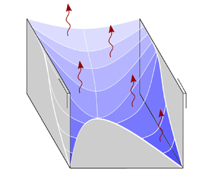
  $\hat {R}$ is depicted in figure 1. The amount of liquid in the reservoir is described using the contact angle on the reservoir sidewall $\theta _R$. The contact line is assumed to be pinned to the top of the reservoir sidewall. As described in Kolliopoulos et al. (Reference Kolliopoulos, Jochem, Johnson, Suszynski, Francis and Kumar2021), the free surface undergoes a transition from that observed in figure 1(a) ( $\lambda \ge \lambda _c$) to that in figure 1(b) ( $\lambda <\lambda _c$). Here, $\lambda =\hat {H}/\hat {W}$ is the channel aspect ratio and $\lambda _c=(1-\sin \theta _0)/2\cos \theta _0$ is the aspect ratio at which the circular upper meniscus contacts the bottom of the rectangular channel while being attached to the top of the channel sidewalls with an equilibrium contact angle $\theta _0$.

Figure 1. Schematic of liquid undergoing capillary flow in an open rectangular channel connected to a circular reservoir for aspect ratios (a)  $\lambda \ge \lambda _c$ and (b) $\lambda <\lambda _c$. Here, $\beta =\arctan (\cos \theta /\cos \theta _0)$ and the finger length is $\tilde {z}_T-\tilde {z}_M$.
Each regime is described using the liquid height  $\hat {a}$ and the contact angle $\theta$ on the channel sidewall. For $\lambda \ge \lambda _c$ (figure 1a), the free-surface morphology is divided into three regimes along the channel length: meniscus deformation $[0,\hat {z}_D]$, meniscus recession $[\hat {z}_D,\hat {z}_M]$ and corner flow $[\hat {z}_M,\hat {z}_T]$. In the meniscus-deformation regime, the upper meniscus curvature at the channel inlet is matched to the liquid–air interface curvature in the reservoir and the upper meniscus curvature increases down the channel length until $\theta (\hat {z}_D,\hat {t})=\theta _0$, while the liquid remains pinned to the top of the channel sidewall $\hat {a}=\hat {H}$.
In the meniscus-recession regime, the contact angle on the sidewall remains constant at  $\theta =\theta _0$ and the liquid height recedes down the sidewall until the upper meniscus contacts the channel bottom $\hat {a}(\hat {z}_M,\hat {t})=\hat {W}\lambda _c$. At this point, the contact angle on the bottom is assumed to reach $\theta _0$ instantaneously. This is the simplest possible assumption, implies a neglect of contact-angle hysteresis, and works well in describing experiments in the absence of evaporation (Kolliopoulos et al. Reference Kolliopoulos, Jochem, Johnson, Suszynski, Francis and Kumar2021). Subsequently, the flow splits into the channel corners, leading to the corner-flow regime. Here, the contact angle on the sidewall and bottom remains constant at $\theta =\theta _0$ and the liquid height further recedes down the sidewall from $\hat {a}(\hat {z}_M,\hat {t})=\hat {W}\lambda _c$ to $\hat {a}(\hat {z}_T,\hat {t})=0$ at the finger tip.
For  $\lambda <\lambda _c$ (figure 1b) the free-surface morphology is also divided into three regimes: meniscus deformation $[0,\hat {z}_M]$, corner transition $[\hat {z}_M,\hat {z}_C]$ and corner flow $[\hat {z}_C,\hat {z}_T]$. In the meniscus-deformation regime, the liquid is pinned to the top of the sidewall ( $\hat {a}=\hat {H}$). The upper meniscus curvature at the channel inlet is matched to the liquid–air interface curvature in the reservoir and the upper meniscus curvature increases down the channel length until $\theta (\hat {z}_M,\hat {t})=\theta _C$ when the upper meniscus touches the channel bottom.
Upon contact with the channel bottom, the contact angle there is assumed to reach  $\theta _0$ instantaneously. The upper meniscus splits into the channel corners, yielding the corner-transition regime. During this stage, the liquid remains pinned to the top of the sidewall ( $\hat {a}=\hat {H}$). To conserve mass, the contact angle at the sidewall $\theta (\hat {z}_M,\hat {t})$ must change from $\theta _C$ to another value denoted $\theta _T$. The contact angle on the sidewall decreases down the channel length until $\theta (\hat {z}_C,\hat {t})=\theta _0$, at which point the flow transitions to the corner-flow regime. Here, $\theta =\theta _0$ and the liquid depins from the top of the sidewall and decreases until $\hat {a}(\hat {z}_T,\hat {t})=0$.
In the following sections we develop a mathematical model for capillary flow of a liquid solution with evaporation considering both  $\lambda \ge \lambda _c$ (figure 1a) and $\lambda <\lambda _c$ (figure 1b), and account for the finite-size reservoir used in experiments (Lade et al. Reference Lade, Jochem, Macosko and Francis2018).
2.2. Hydrodynamics
Mass and momentum conservation for an incompressible Newtonian liquid are governed by
 \begin{align} \boldsymbol{\widehat{\nabla}} \boldsymbol{\cdot} \boldsymbol{\hat{u}}=0 \quad \text{and} \quad \hat{\rho} \left[\frac{\partial \boldsymbol{\hat{u}}}{\partial \hat{t}}+ (\boldsymbol{\hat{u}} \boldsymbol{\cdot} \boldsymbol{\widehat{\nabla}})\boldsymbol{\hat{u}}\right]={-}\boldsymbol{\widehat{\nabla}}\hat{p} +\hat{\mu} \widehat{\nabla}^2 \boldsymbol{\hat{u}} + \hat{\rho} \boldsymbol{\hat{g}}, \end{align}
where  $\boldsymbol {\hat {u}}=(\hat {u},\hat {v},\hat {w})$ is the velocity in Cartesian coordinates $(\hat {x},\hat {y},\hat {z})$, $\hat {p}$ is the liquid pressure and $\boldsymbol {\hat {g}}=(\hat {g}_x,\hat {g}_y,\hat {g}_z)$ is the gravitational acceleration. Along the channel walls, the no-slip and no-penetration conditions require $\boldsymbol {\hat {u}}=0$. The boundary conditions for the jump in normal, transverse tangential, and axial tangential stresses across the liquid–air interface $\hat {h}(\hat {x},\hat {z},\hat {t})$ are
 \begin{align} [\![\boldsymbol{n}\boldsymbol{\cdot} \hat{\boldsymbol{T}}\boldsymbol{\cdot}\boldsymbol{n}]\!]=\hat{\sigma} (\boldsymbol{\widehat{\nabla}}_s \boldsymbol{\cdot} \boldsymbol{n}), \quad [\![\boldsymbol{t}_1\boldsymbol{\cdot} \hat{\boldsymbol{T}}\boldsymbol{\cdot}\boldsymbol{n}]\!]=\boldsymbol{t}_1 \boldsymbol{\cdot} \boldsymbol{\widehat{\nabla}}_s \hat{\sigma}, \quad \text{and} \quad [\![\boldsymbol{t}_2\boldsymbol{\cdot} \hat{\boldsymbol{T}}\boldsymbol{\cdot}\boldsymbol{n}]\!]=\boldsymbol{t}_2 \boldsymbol{\cdot} \boldsymbol{\widehat{\nabla}}_s \hat{\sigma}. \end{align}
Here,  $\hat {\boldsymbol {T}}=-\hat {p}\boldsymbol {I}+\hat {\mu }[\boldsymbol {\widehat {\nabla }}\boldsymbol {\hat {u}}+(\boldsymbol {\widehat {\nabla }}\boldsymbol {\hat {u}})^{\rm T}]$ is the stress tensor, $\boldsymbol {I}$ is the identity tensor, $\boldsymbol {\widehat {\nabla }}_s=\boldsymbol {\widehat {\nabla }}-\boldsymbol {n}(\boldsymbol {n}\boldsymbol {\cdot }\boldsymbol {\widehat {\nabla }})$ is the surface-gradient operator, $\boldsymbol {n}$ is the unit outward normal vector and $\boldsymbol {t}_1$, $\boldsymbol {t}_2$ are the two unit tangent vectors to the interface in the transverse and axial directions, respectively. These vectors are given by
 \begin{equation} \boldsymbol{n}=\frac{(-\hat{h}_{\hat{x}},1,-\hat{h}_{\hat{z}})}{\sqrt{1+\hat{h}_{\hat{x}}^2+\hat{h}_{\hat{z}}^2}},\quad \boldsymbol{t}_1=\frac{(1+\hat{h}_{\hat{z}}^2,\hat{h}_{\hat{x}},-\hat{h}_{\hat{x}}\hat{h}_{\hat{z}})}{\sqrt{(1+\hat{h}_{\hat{z}}^2)^2 +\hat{h}_{\hat{x}}^2 +\hat{h}_{\hat{x}}^2\hat{h}_{\hat{z}}^2}},\quad \boldsymbol{t}_2=\frac{(0,\hat{h}_{\hat{z}},1)}{\sqrt{1+\hat{h}_{\hat{z}}^2}}. \end{equation}
Equations (2.1a) are rendered dimensionless using the following scalings:
 \begin{gather} \left. \begin{gathered} (\hat{x},\hat{y},\hat{z})=\hat{L}(\epsilon x,\epsilon y, z), \enspace (\hat{u},\hat{v},\hat{w})=\hat{U}(\epsilon u,\epsilon v,w), \enspace (\hat{g}_x,\hat{g}_y,\hat{g}_z)=\hat{g}(g_x,g_y,g_z),\\ \hat{t}=(\hat{L}/\hat{U})t, \enspace \epsilon=\hat{H}/\hat{L}, \quad \hat{U}=\epsilon\hat{\sigma}_0/\hat{\mu}_0, \enspace \hat{p}=(\hat{\mu}_0 \hat{U}/\epsilon \hat{H})p, \enspace \hat{\mu}=\hat{\mu}_0M, \enspace \hat{\sigma}=\hat{\sigma}_0\varSigma,\\ \end{gathered} \right\} \end{gather}
where  $\epsilon$ is the ‘slenderness’ parameter, $\hat {U}$ is the viscocapillary velocity, $\hat {\mu }_0$ is the solvent viscosity, $\hat {\sigma }_0$ is the solvent surface tension and $M$ and $\varSigma$ are the dimensionless solution viscosity and surface tension, respectively, defined in § 2.6. The dimensionless numbers that arise are the Reynolds number $Re=\hat {\rho } \hat {U}\hat {H}/\hat {\mu }_0$ (ratio of inertial to viscous forces), the capillary number $Ca=\hat {\mu }_0\hat {U}/\epsilon \hat {\sigma }_0$ (ratio of viscous to surface-tension forces) and the Bond number $Bo=\hat {\rho } \hat {g}\hat {H}^2/\hat {\sigma }_0$ (ratio of gravitational to surface-tension forces). Note that $Ca=1$ based on our choice of $\hat {U}$.
In the limits where  $\epsilon ^2\ll 1$, $\epsilon Re\ll 1$ and $Bo/Ca\ll \epsilon$, (2.1a) reduces to
 \begin{gather} u_x + v_y + w_z =0, \end{gather}
 \begin{gather} p_x = p_y=0, \end{gather}
 \begin{gather} p_z= M(w_{xx} +w_{yy}). \end{gather}
The boundary conditions at the free surface in (2.1b) reduce to
 \begin{gather} p-p_{V,T}={-}\frac{\varSigma}{Ca} \left[\frac{h_{x}}{(1+h_{x}^2)^{1/2}}\right]_x ={-}\frac{\varSigma}{Ca} \kappa, \end{gather}
 \begin{gather} (1-h_x^2)(v_x+u_y) +2h_x({-}u_x+v_y)\,{-}\,(1-h_x^2)h_z w_x \,{-}\, 2h_xh_z w_y\nonumber\\ \hspace{-8pc}={-}h_xh_z(1+h_x^2)^{1/2}\frac{\varSigma_z}{MCa}, \end{gather}
 \begin{gather} w_y-h_x w_x = \frac{\varSigma_z}{MCa}, \end{gather}
where  $p_{V,T}$ is the total pressure in the vapour phase and is assumed constant. Since the leading-order pressure term is independent of $(x,y)$ according to (2.4b), the leading-order curvature term $\kappa$ only depends on $(z,t)$ according to (2.5a).
We note two things about these reduced equations. First, the interface shape at a given  $z$-position is determined by capillary statics (Yang & Homsy Reference Yang and Homsy2006), as can be seen from (2.5a). As a consequence, contact angles can be imposed as boundary conditions without having to specify a slip law. The interface shape slowly varies in the $z$-direction via an evolution equation to be presented in § 2.7. This approach is expected to hold for $\hat {\mu }_0 \hat {U}/\hat {\sigma }_0 \ll 1$. Second, because of the problem we are considering and our choice of variables, $h_x$ is ${O}(1)$, so the $h_x^2$ terms are retained.
As shown by Kolliopoulos et al. (Reference Kolliopoulos, Jochem, Johnson, Suszynski, Francis and Kumar2021), using a condition for the contact-line location on the solid wall, a symmetry condition, and the definition of the contact angle on the sidewall, expressions for  $p(z,t)$ and $h(x,z,t)$ are obtained by integrating (2.5a) twice with respect to $x$, leading to
 \begin{gather} \text{meniscus deformation} \quad \begin{cases} p={-}2\varSigma\lambda\cos\theta(z,t) + p_{V,T}, \\ h=1+\dfrac{\tan\theta(z,t)}{2\lambda}-\left[\dfrac{1}{4\lambda^2\cos^2\theta(z,t)}-x^2\right]^{1/2} , \\ A = \dfrac{1}{4\lambda^2}\left[4\lambda-\dfrac{{\rm \pi}/2-\theta(z,t)}{\cos^2\theta(z,t)}+\tan\theta(z,t)\right], \end{cases} \end{gather}
 \begin{gather} \text{meniscus recession} \quad \begin{cases} p={-}2\varSigma\lambda\cos\theta_0 + p_{V,T}, \\ h=a(z,t)+\dfrac{\tan\theta_0}{2\lambda}-\left[\dfrac{1}{4\lambda^2\cos^2\theta_0}-x^2\right]^{1/2}, \\ A = \dfrac{1}{4\lambda^2}\left[4\lambda a(z,t)-\dfrac{{\rm \pi}/2-\theta_0}{\cos^2\theta_0}+\tan\theta_0\right], \end{cases} \end{gather}
 \begin{gather} \text{corner transition} \quad \begin{cases} p={-}\varSigma[\cos\theta_0-\sin\theta(z,t)] + p_{V,T}, \\ h=\dfrac{\cos\theta\cos\beta}{\cos(\theta+\beta)}-\left[\left(\dfrac{\sin\beta}{\cos(\theta+\beta)}\right)^2-\left(\dfrac{\cos\theta\sin\beta}{\cos(\theta+\beta)}-x-\dfrac{1}{2\lambda}\right)^2\right]^{1/2}, \\ A = \dfrac{B(\theta,\theta_0)}{(\cos\theta_0-\sin\theta)^2}, \end{cases} \end{gather}
 \begin{gather} \text{corner flow} \quad \begin{cases} p={-}\dfrac{\varSigma[\cos\theta_0-\sin\theta_0]}{a(z,t)} + p_{V,T}, \\ h=\dfrac{a\cos\theta_0\cos\frac{\rm \pi}{4}}{\cos(\theta_0+\frac{\rm \pi}{4})}-\left[\left(\dfrac{a\sin\frac{\rm \pi}{4}}{\cos(\theta_0+\frac{\rm \pi}{4})}\right)^2-\left(\dfrac{a\cos\theta_0\sin\frac{\rm \pi}{4}}{\cos(\theta_0+\frac{\rm \pi}{4})}-x-\dfrac{1}{2\lambda}\right)^2\right]^{1/2}, \\ A = \dfrac{a^2B(\theta_0,\theta_0)}{(\cos\theta_0-\sin\theta_0)^2}, \end{cases} \end{gather}
where  $\beta =\arctan (\cos \theta /\cos \theta _0)$ and $A=2\int _{x_1}^{x_2} h\,\mathrm {d}\kern0.7pt x$ is the dimensionless liquid cross-sectional area. Note that $\theta$ and $a$ in (2.6) are dependent on $(z,t)$. The integration bounds for each regime are
 \begin{equation} \left. \begin{aligned} & \text{meniscus deformation:} \quad x_1 =0 \quad \text{and} \quad x_2=\dfrac{1}{2\lambda},\\ & \text{meniscus recession:} \quad x_1 =0 \quad \text{and} \quad x_2=\dfrac{1}{2\lambda},\\ & \text{corner transition:} \quad x_1 = \dfrac{1}{2\lambda} -\dfrac{\cos\theta-\sin\theta_0}{\cos\theta_0-\sin\theta} \quad \text{and} \quad x_2=\dfrac{1}{2\lambda},\\ & \text{corner flow:} \quad x_1 =\dfrac{1}{2\lambda} -a\dfrac{\cos\theta-\sin\theta_0}{\cos\theta_0-\sin\theta} \quad \text{and} \quad x_2=\dfrac{1}{2\lambda}. \end{aligned} \right\} \end{equation}
 The geometric function  $B(\theta,\theta _0)$ in the expressions for $A$ is given by
 \begin{equation} B(\theta,\theta_0)=\theta+\theta_0 -{\rm \pi}/2-\cos\theta(\sin\theta-\cos\theta_0)+\cos\theta_0(\cos\theta-\sin\theta_0). \end{equation}
Equations (2.6) were also used by Kolliopoulos et al. (Reference Kolliopoulos, Jochem, Johnson, Suszynski, Francis and Kumar2021) and in other previous studies (Romero & Yost Reference Romero and Yost1996; Weislogel & Lichter Reference Weislogel and Lichter1998; Tchikanda, Nilson & Griffiths Reference Tchikanda, Nilson and Griffiths2004; Weislogel & Nardin Reference Weislogel and Nardin2005; Nilson et al. Reference Nilson, Tchikanda, Griffiths and Martinez2006; Yang & Homsy Reference Yang and Homsy2006; White & Troian Reference White and Troian2019).
2.3. Evaporation
We assume the liquid is in contact with a gas phase having ambient temperature  $\hat {T}_A$ and relative humidity $R_H$. The gas phase consists of saturated vapour or a mixture of solvent vapour and inert gas (e.g. air), and its velocity is assumed to be negligible. We assume the gas phase density $\hat {\rho }_V$, viscosity $\hat {\mu }_V$, and thermal conductivity $\hat {k}_V$, are much smaller than their liquid counterparts (Burelbach, Bankoff & Davis Reference Burelbach, Bankoff and Davis1988), and the temperature across the liquid–air interface is continuous (Sefiane & Ward Reference Sefiane and Ward2007). These assumptions allow us to describe evaporation using a kinetically limited model focusing only on the liquid phase.
A kinetically limited model is chosen instead of a diffusion-limited model (Gambaryan- Roisman Reference Gambaryan-Roisman2019) for three reasons. First, a kinetically limited model is expected to be more accurate at describing evaporating flow of liquid solutions since the presence of solute at the free surface makes the rate-limiting step more likely to be in the liquid phase (Cazabat & Guéna Reference Cazabat and Guéna2010). Second, kinetically limited models have proven useful in interpreting experiments involving evaporation into an unsaturated environment when the vapour diffuses rapidly away from the evaporating interface even though they were originally developed for evaporation into a saturated environment (Murisic & Kondic Reference Murisic and Kondic2011). Third, a kinetically limited model does not require keeping track of the solvent concentration in the vapour phase, which makes it computationally simpler while still providing qualitatively accurate predictions (Ajaev Reference Ajaev2005; Murisic & Kondic Reference Murisic and Kondic2011). We note that, although a kinetically limited model is expected to provide qualitatively accurate predictions, it is unlikely to produce quantitatively accurate predictions for situations where evaporation is diffusion limited.
Evaporation is modelled using the non-equilibrium Hertz–Knudsen relation based on the kinetic theory of gases (Plesset & Prosperetti Reference Plesset and Prosperetti1976; Moosman & Homsy Reference Moosman and Homsy1980). The evaporative mass flux is described using
 \begin{equation} \hat{j}=\alpha_E\hat{p}_{V}\left(\frac{\hat{R}_g \hat{T}|_{\hat{h}}}{2 {\rm \pi}}\right)^{1/2}\left(\frac{\hat{p}_{V,e}}{\hat{p}_{V}}-1\right), \end{equation}
where  $\alpha _E$ is the thermal accommodation coefficient, $\hat {R}_g$ is the gas constant per unit mass, $\hat {T}|_{\hat {h}}$ is the local liquid–air interface temperature, $\hat {p}_{V}$ is the partial pressure of solvent in the vapour phase and $\hat {p}_{V,e}$ is the equilibrium solvent vapour pressure. Note that we have assumed the thermal accommodation coefficients for evaporation and condensation are equal to $\alpha _E$. Physically, $\alpha _E$ can be thought of as a barrier to phase change, with $\alpha _E=1$ corresponding to no barrier and $\alpha _E=0$ corresponding to no phase change (Persad & Ward Reference Persad and Ward2016). Prior studies have reported values of $\alpha _E$ that vary over several orders of magnitude from ${O}(10^{-6})$ to ${O}(1)$ (Marek & Straub Reference Marek and Straub2001; Murisic & Kondic Reference Murisic and Kondic2011). In this work, we use the accommodation coefficient as a fitting parameter when comparing with experiments, similar to Murisic & Kondic (Reference Murisic and Kondic2011).
According to equilibrium thermodynamics (Moosman & Homsy Reference Moosman and Homsy1980; Ajaev & Homsy Reference Ajaev and Homsy2001; Ajaev Reference Ajaev2005) we can write
 \begin{equation} \ln\left(\frac{\hat{p}_{V,e}}{\hat{p}_V}\right)=\frac{\hat{\mathcal{L}}}{\hat{R}_g}\left(\frac{1}{\hat{T}_V}-\frac{1}{\hat{T}|_{\hat{h}}}\right)+\frac{\hat{p}-\hat{p}_V}{\hat{\rho} \hat{R}_g \hat{T}|_{\hat{h}}}, \end{equation}
where  $\hat {\mathcal {L}}$ is the latent heat and $\hat {T}_V$ is the vapour temperature. The partial pressure of solvent in the vapour phase is calculated using $\hat {p}_V = R_H \hat {p}_S(\hat {T}_A)$ (Cazabat & Guéna Reference Cazabat and Guéna2010; Murisic & Kondic Reference Murisic and Kondic2011), where $R_H$ is the relative humidity, which ranges from 0 to 1, and $\hat {p}_S(\hat {T}_{A})$ is the saturation pressure corresponding to the ambient temperature $\hat {T}_{A}$. Both $\hat {p}_V$ and $\hat {T}_{A}$ in the vapour phase are assumed uniform and constant. The partial pressure of the solvent $\hat {p}_V$ is then used to calculate the vapour temperature $\hat {T}_V$ using the Clausius–Clapeyron equation (Murisic & Kondic Reference Murisic and Kondic2011). Note that for $R_H=1$ (which corresponds to a vapour phase saturated with solvent), $\hat {p}_V=\hat {p}_S$ and $\hat {T}_V=\hat {T}_A$.
We rescale (2.10) and (2.9) using
 \begin{equation} \hat{p}=(\hat{\mu}_0 \hat{U}/\epsilon \hat{H})p, \quad \hat{T} = \hat{T}_V+T\Delta\hat{T}, \quad \Delta\hat{T}=\hat{T}_W-\hat{T}_V, \quad \text{and} \quad \hat{j}=(\hat{k}\Delta\hat{T}/\hat{\mathcal{L}}\hat{H})j, \end{equation}
where  $\hat {T}_W$ is the temperature of the channel walls, and substitute (2.10) into (2.9), assuming $\ln (\hat {p}_{V,e}/\hat {p}_V)\approx \hat {p}_{V,e}/\hat {p}_V -1$ and $\sqrt {\hat {T}|_{\hat {h}}} \approx \sqrt {\hat {T}_V}$. The resulting expression for the evaporative mass flux is
 \begin{equation} Kj=\delta (p-p_V)+T|_h, \end{equation}
where  $K=\hat {k}\sqrt {2{\rm \pi} \hat {R}_g^3\hat {T}_V^5}/\hat {p}_V\hat {\mathcal {L}}^2\hat {H}\alpha _E$ is the Knudsen number (ratio of interfacial to bulk heat transfer resistance), which is essentially the inverse of the Biot number, and $\delta =\hat {\mu }_0\hat {U}\hat {T}_V/\hat {\rho }\epsilon \hat {H}\hat {\mathcal {L}}\Delta \hat {T}$ accounts for the effects of pressure variation on the local interface temperature (Ajaev Reference Ajaev2005). From (2.12) it can be seen that the evaporative mass flux $j$ is proportional to deviations from $p_V$ and $\hat {T}_V$. Note that $\delta$ is typically ${O}(10^{-4}-10^{-6})$ compared with $T|_h$ which is ${O}(1)$, so contributions of the $\delta (p-p_V)$ term in (2.12) are typically neglected (Markos et al. Reference Markos, Ajaev and Homsy2006; Murisic & Kondic Reference Murisic and Kondic2011). However, these contributions become significant near the finger tip as $a\rightarrow 0$, where $p\rightarrow -\infty$ as seen in (2.6d).
2.4. Energy transport
Energy conservation is governed by
 \begin{equation} \hat{\rho}\hat{C}_p\left[\frac{\partial \hat{T}}{\partial \hat{t}} + \boldsymbol{\hat{u}} \boldsymbol{\cdot} \boldsymbol{\widehat{\nabla}}\hat{T}\right] = \hat{k} \widehat{\nabla}^2 \hat{T}. \end{equation}
For simplicity, we consider the limiting case where heat conduction in the channel walls is neglected, and assume that the channel walls are held at a constant temperature  $\hat {T}_W$. The energy balance at the liquid–air interface is
 \begin{equation} \hat{\mathcal{L}}\hat{j}={-}\boldsymbol{n} \boldsymbol{\cdot} \hat{k} \boldsymbol{\widehat{\nabla}}\hat{T}. \end{equation}
We render (2.13) dimensionless using the scalings in (2.3) and (2.11a–d). The dimensionless numbers that arise are the Reynolds number  $Re$ (see § 2.2) and the Prandtl number $Pr=\hat {\mu }_0\hat {C}_p/\hat {k}$ (ratio of momentum to thermal diffusivity).
In the limits of  $\epsilon ^2\ll 1$ and $\epsilon Re Pr\ll 1$, the leading-order energy-transport equation is
 \begin{equation} T_{xx} + T_{yy} = 0, \end{equation}
subject to
 \begin{equation} T = 1 \quad \text{at solid boundaries} \quad \text{and} \quad j (1+h_x^2)^{1/2} = h_xT_x - T_y \quad \text{at free surface}, \end{equation}
where  $j$ is determined using (2.12). The total evaporative mass flux for a given channel cross-section is defined as
 \begin{equation} \tilde{J}=\int_S j\,\mathrm{d}S = 2\int_{x_1}^{x_2} j (1+h_x^2)^{1/2} \,\mathrm{d} x, \end{equation}
where  $x_1$ and $x_2$ are given by (2.7). The liquid–air interface arc length is given by
 \begin{equation} S = \begin{cases} \dfrac{{\rm \pi} - 2\theta}{\lambda\cos\theta} \quad \text{in meniscus-deformation regime}, \\ \dfrac{{\rm \pi} - 2\theta_0}{\lambda\cos\theta_0} \quad \text{in meniscus-recession regime}, \\ \dfrac{(2{\rm \pi} - 4\theta-4\beta)\sin\beta}{\cos(\theta+\beta)} \quad \text{in corner-transition regime}, \\ \dfrac{({\rm \pi} - 4\theta)a\sin{\rm \pi}/4}{\cos(\theta+{\rm \pi}/4)} \quad \text{in corner-flow regime}, \end{cases} \end{equation}
where  $\theta$ and $a$ are dependent on $(z,t)$ and the cross-sectional-averaged dimensionless temperature is defined as
 \begin{equation} \bar{T}=\frac{1}{A}\int_A T\,\mathrm{d}A, \end{equation}
where  $A$ is the liquid cross-sectional area from (2.6).
2.5. Solute transport
A convection–diffusion equation governs the transport of solute
 \begin{equation} \frac{\partial c}{\partial \hat{t}} + \boldsymbol{\hat{u}} \boldsymbol{\cdot} \boldsymbol{\widehat{\nabla}} c= \hat{D} \widehat{\nabla}^2 c, \end{equation}
where  $c$ is the solute concentration (mass fraction) and $\hat {D}$ is the diffusion coefficient, which is assumed to be constant. We impose no-flux boundary conditions
 \begin{gather} \hat{D}(\boldsymbol{n}\boldsymbol{\cdot} \boldsymbol{\widehat{\nabla}})c = 0 \quad \text{at solid boundaries}, \end{gather}
 \begin{gather} \hat{D}(\boldsymbol{n}\boldsymbol{\cdot} \boldsymbol{\widehat{\nabla}})c = c(\boldsymbol{\hat{u}}-\boldsymbol{\hat{u}_I}) \boldsymbol{\cdot} \boldsymbol{n} = c \hat{j}/\hat{\rho} \quad \text{at free surface}, \end{gather}
where  $\boldsymbol {\hat {u}_I}$ is the liquid–air interface velocity and $\hat {j}$ is the local evaporative mass flux. Using the scalings in (2.3), (2.19a) becomes
 \begin{equation} \epsilon^2 Pe (c_t + uc_x + v c_y + wc_z) = c_{xx} + c_{yy}+\epsilon^2 c_{zz}, \end{equation}
where  $Pe=\hat {U}\hat {L}/\hat {D}$ is the Péclet number (ratio of convective to diffusive transport rates). Similarly, the no-flux boundary conditions become
 \begin{gather} (\boldsymbol{n}\boldsymbol{\cdot} \boldsymbol{\nabla})c = 0 \quad \text{at solid boundaries}, \end{gather}
 \begin{gather} -h_x c_x + c_y - \epsilon^2 h_z c_z = \epsilon^2 Pe cEj(1+h_x^2)^{1/2} \quad \text{at free surface}, \end{gather}
where  $E=\hat {k}\Delta \hat {T}/\hat {\rho }\hat {\mathcal {L}}\hat {H}\epsilon \hat {U}$ is the evaporation number (ratio of characteristic capillary to evaporation times).
To simplify (2.20a) further, we assume solute transport in the  $x$ and $y$ directions is dominated by diffusion ( $\epsilon ^2 Pe \ll 1$). As proposed by Jensen & Grotberg (Reference Jensen and Grotberg1993), we asymptotically expand the concentration in terms of $\epsilon ^2 Pe$, obtaining $c(x,y,z,t) = c_0(z,t) + \epsilon ^2 Pe c_1(x,y,z,t)$, where we assume $\int _A c_1 \, \mathrm {d}A=0$. This allows us to define the cross-sectional-averaged concentration as
 \begin{equation} \bar{c}= \frac{1}{A}\int_A c \,\mathrm{d}A = c_0(z,t). \end{equation}
We apply cross-sectional averaging to (2.20a) and replace the  $c_1$ terms using the no-flux condition at the free surface in (2.20c). In the limit of $\epsilon ^2 \ll 1$, we obtain the following evolution equation for $\bar {c}$:
 \begin{equation} \bar{c}_{t} + \bar{w} \bar{c}_{z} = \frac{1}{PeA}(A\bar{c}_{z})_z + \frac{\bar{c}}{A}E\tilde{J}, \end{equation}
where  $\bar {w}$ is the cross-sectional-averaged velocity (which will be obtained from (2.28)), $A$ is the dimensionless cross-sectional area from (2.6), and $\tilde {J}$ is the total cross-sectional evaporative mass flux in a given channel cross-section from (2.16).
2.6. Constitutive equations for viscosity and surface tension
The constitutive equations for viscosity  $M$ and surface tension $\varSigma$ depend on the liquid solution we choose to study. In this work, we use aqueous poly(vinyl alcohol) (PVA) solutions and compare model predictions with capillary-flow experiments conducted by Lade et al. (Reference Lade, Jochem, Macosko and Francis2018). An empirical model proposed by Patton (Reference Patton1964) is used to capture the dependence of the viscosity on $\bar {T}$ and $\bar {c}$ through
 \begin{equation} \log M = \dfrac{\bar{c}}{k_a(\bar{T})+\bar{c}k_b(\bar{T})}, \end{equation}
where
 \begin{equation} \left. \begin{aligned} k_a(\bar{T}) & = 1.28\times10^{{-}5}(\hat{T}_V+\bar{T}\Delta\hat{T})+1.59\times10^{{-}2},\\ k_b(\bar{T}) & = 3.83\times10^{{-}4}(\hat{T}_V+\bar{T}\Delta\hat{T})-2.47\times10^{{-}2}. \end{aligned} \right\} \end{equation}
The  $k_a(\bar {T})$ and $k_b(\bar {T})$ functions were reported by Lade et al. (Reference Lade, Jochem, Macosko and Francis2018) after fitting the empirical model to rheological data of PVA solutions for a range of temperatures and concentrations. In (2.23a), increasing the solute concentration can increase the viscosity by orders of magnitude, and increasing the temperature decreases the viscosity but does not change its order of magnitude. Similar models can be used to describe any solution or colloidal suspension where the shear viscosity is the dominant rheological parameter.
The effects of  $\bar {T}$ and $\bar {c}$ on the surface tension are modelled using
 \begin{equation} \varSigma = 1 - Ma_c\bar{c}^{1/2} - Ma_T \bar{T}, \end{equation}
where  $Ma_c=\hat {\gamma }_c \epsilon /\hat {\mu }_0 \hat {U}$ is the solutal Marangoni number and $Ma_T=\hat {\gamma }_T\Delta \hat {T}\epsilon /\hat {\mu }_0 \hat {U}$ is the thermal Marangoni number, which are ratios of surface-tension-gradient forces to viscous forces, and $\hat {\gamma }_c$ and $\hat {\gamma }_T$ are experimentally obtained constants. We assume the temperature at the liquid–air interface does not deviate much from the vapour temperature, which allows us to write the surface tension as a linear function of $\bar {T}$ (Burelbach et al. Reference Burelbach, Bankoff and Davis1988; Gramlich et al. Reference Gramlich, Kalliadasis, Homsy and Messer2002; Ajaev Reference Ajaev2005; Craster, Matar & Sefiane Reference Craster, Matar and Sefiane2009). Many prior studies assume a dilute solution and use a linearized surface-tension dependence on the concentration (e.g. Lam & Benson Reference Lam and Benson1970; Pham, Cheng & Kumar Reference Pham, Cheng and Kumar2017); this would yield results that are qualitatively similar to those obtained using (2.24). Comparison of the empirical models in (2.23a) and (2.24) with the experimental results of Lade et al. (Reference Lade, Jochem, Macosko and Francis2018) is found in the supplementary material available at https://doi.org/10.1017/jfm.2022.140.
2.7. Liquid height evolution
We begin with the no-flux boundary condition at the free surface given by
 \begin{equation} (\boldsymbol{\hat{u}}-\boldsymbol{\hat{u}_I}) \boldsymbol{\cdot} \boldsymbol{n} = \hat{j}/\hat{\rho}, \end{equation}
where the velocity of the liquid–air interface is  $\boldsymbol {\hat {u}_I}=(0,\hat {h}_{\hat {t}},0)$. Using the scalings in (2.3) and (2.11a–d), (2.25) becomes
 \begin{equation} {-}uh_x+v-wh_z-h_t=Ej(1+h_x^2+\epsilon^2h_z^2)^{1/2}. \end{equation}
 We apply cross-sectional averaging to the mass conservation equation (2.4a) and replace the  $u$ and $v$ terms using (2.26), thus obtaining
 \begin{equation} A_t={-}(\bar{w} A)_z - E\tilde{J}, \end{equation}
where for each regime, the dimensionless liquid cross-sectional area  $A=2\int _{x_1}^{x_2} h\,\mathrm {d} x$ is given by (2.6), $\bar {w}=A^{-1}\int _A w\,\mathrm {d}A$ is the cross-sectional-averaged velocity and $\tilde {J}$ is the total evaporative mass flux in a given channel cross-section from (2.16). Equation (2.27) is the mass-balance equation derived by Lenormand & Zarcone (Reference Lenormand and Zarcone1984), relating the time derivative of the dimensionless liquid cross-sectional area $A$ to the gradient in the dimensionless flux $Q=\int _A w\,\mathrm {d}A =\bar {w} A$, with an additional term accounting for mass lost due to solvent evaporation.
The velocity in (2.27) can be decomposed as follows:
 \begin{equation} \bar{w} = \bar{w}_{ca} + \bar{w}_{cg} + \bar{w}_{tg}, \end{equation}
where each contribution in each regime (figure 1) is expressed in (2.29). Each component corresponds to a different mechanism acting on the liquid to drive flow. Here,  $\bar {w}_{ca}$ is the velocity due to capillary effects, while $\bar {w}_{cg}$ and $\bar {w}_{tg}$ correspond to the effects of Marangoni stresses. Specifically, $\bar {w}_{cg}$ is due to solute concentration gradients and $\bar {w}_{tg}$ is due to thermal gradients. For each regime these contributions are given by
 $$\begin{gather} \bar{w}_{ca} ={-}\dfrac{\bar{U}^c_{D}}{M}p_z, \quad \bar{w}_{cg} = \dfrac{\bar{U}^g_{D}}{M}\dfrac{\partial\varSigma}{\partial\bar{c}}\bar{c}_z, \quad \bar{w}_{tg} = \dfrac{\bar{U}^g_{D}}{M}\dfrac{\partial\varSigma}{\partial\bar{T}}\bar{T}_z, \quad \text{meniscus deformation}, \end{gather}$$
 $$\begin{gather}\bar{w}_{ca} ={-}\dfrac{\bar{U}^c_{R}}{M}p_z, \quad \bar{w}_{cg} = \dfrac{\bar{U}^g_{R}}{M}\dfrac{\partial\varSigma}{\partial\bar{c}}\bar{c}_z, \quad \bar{w}_{tg} = \dfrac{\bar{U}^g_{R}}{M}\dfrac{\partial\varSigma}{\partial\bar{T}}\bar{T}_z, \quad \text{meniscus recession}, \end{gather}$$
 $$\begin{gather}\bar{w}_{ca} ={-}\dfrac{\bar{U}^c_{T}}{M}p_z, \quad \bar{w}_{cg} = \dfrac{\bar{U}^g_{T}}{M}\dfrac{\partial\varSigma}{\partial\bar{c}}\bar{c}_z, \quad \bar{w}_{tg} = \dfrac{\bar{U}^g_{T}}{M}\dfrac{\partial\varSigma}{\partial\bar{T}}\bar{T}_z, \quad \text{corner transition}, \end{gather}$$
 $$\begin{gather}\bar{w}_{ca} ={-}a^2\dfrac{\bar{U}^c_{C}}{M}p_z, \quad \bar{w}_{cg} = \dfrac{\bar{U}^g_{C}}{M}\dfrac{\partial\varSigma}{\partial\bar{c}}\bar{c}_z, \quad \bar{w}_{tg} = a\dfrac{\bar{U}^g_{C}}{M}\dfrac{\partial\varSigma}{\partial\bar{T}}\bar{T}_z, \quad \text{corner flow}, \end{gather}$$
where  $\bar {U}^c_{i}$ and $\bar {U}^g_{i}$ are rescaled cross-sectional-averaged dimensionless velocities, with the subscript $i$ being equal to $D,R,T$ or $C$ for the meniscus-deformation, meniscus-recession, corner-transition and corner-flow regimes, respectively. Details of the calculation of $\bar {U}^c_{i}$ and $\bar {U}^g_{i}$ can be found in the supplementary material. The expressions for $M$ and $\varSigma$ are given by (2.23a) and (2.24), respectively.
Consistent with prior studies considering horizontal rectangular channels, we neglect the meniscus-recession regime (i.e.  $z_D=z_M$) where $\bar {w}_{ca}=0$. This is because the transverse curvature gradients are zero (constant $p$ in (2.6b)) and the only contribution to $\bar {w}_{ca}$ is from ${O}(\epsilon ^2)$ axial curvature gradients, which we did not account for. The transition from the meniscus-deformation regime to the corner-flow regime (for $\lambda >\lambda _c$) is treated as a jump in the dimensionless liquid height $a(z,t)$ (Nilson et al. Reference Nilson, Tchikanda, Griffiths and Martinez2006; Kolliopoulos et al. Reference Kolliopoulos, Jochem, Johnson, Suszynski, Francis and Kumar2021).
2.8. Reservoir
Liquid is supplied to the microchannel from a cylindrical reservoir of radius  $\hat {R}$ and height $\hat {H}$, and the liquid–air interface in the reservoir is assumed to be axisymmetric. The channel inlet is assumed to have a negligible influence on the liquid–air interface in the reservoir. The reservoir aspect ratio is $\lambda _R=\hat {H}/\hat {R}$ and the cylindrical coordinates of the reservoir are scaled using $(\hat {r},\hat {y},\phi )=(\hat {R}r,\hat {H} y,\phi )$.
2.8.1. Hydrodynamics
Following a similar procedure to the one described in § 2.2, the normal stress balance in (2.1b) reduces to the Young–Laplace equation,
 \begin{equation} p-p_{V,T}={-}\frac{\varSigma \lambda_R^2}{Ca} \left[\frac{h_{rr}}{(1+\lambda_R^2h_{r}^2)^{3/2}}+\frac{h_r}{r(1+\lambda_R^2h_{r}^2)^{1/2}}\right]. \end{equation}
Using (2.30) in combination with a condition for the contact-line location on the solid wall ( $h=1$, at $r=1$), a symmetry condition at the reservoir centre ( $h_r=0$, at $r=0$) and the definition of the contact angle $\theta _R$ on the solid wall ( $\lambda _Rh_r/[1+\lambda _R^2 h_r^2]^{1/2}=\cos \theta _R$, at $r=1$), we obtain the following leading-order expressions for pressure $p(t)$ and liquid–air interface profile $h(r,t)$ in the reservoir:
 \begin{gather} p={-}2\varSigma\lambda_R\cos\theta_R(t)+p_{V,T}, \end{gather}
 \begin{gather} h=1+\dfrac{\tan\theta_R(t)}{\lambda_R}-\frac{1}{\lambda_R}\left[\dfrac{1}{\cos^2\theta_R(t)}-r^2\right]^{1/2}. \end{gather}
2.8.2. Energy transport
Similar to § 2.4, we consider energy conservation in the limit of  $\lambda _R Re Pr\ll 1$, resulting in
 \begin{equation} \frac{\lambda_R^2}{r}\left(rT_r\right)_r+T_{yy}=0, \end{equation}
subject to
 \begin{equation} T = 1 \quad \text{at solid boundaries}, \quad \text{and} \quad j (1+\lambda_R^2h_r^2)^{1/2} = \lambda_R^2 h_rT_r - T_y \quad \text{at free surface}. \end{equation}
Note that in the limit of  $\lambda _R\rightarrow 0$, (2.32) solved along with (2.12) results in the evaporation models used for axisymmetric droplets and thin films, where $j = (1+\delta (p-p_V))/(K + h)$ (Ajaev & Homsy Reference Ajaev and Homsy2001; Ajaev Reference Ajaev2005; Pham & Kumar Reference Pham and Kumar2017, Reference Pham and Kumar2019).
The dimensionless total evaporative mass flux for a given reservoir cross-section is defined as
 \begin{equation} \tilde{J}_R=\int_{S_R} j\,\mathrm{d}S_R=\int_0^1 j (1+\lambda_R^2h_r^2)^{1/2}r\,\mathrm{d}r. \end{equation}
The liquid–air interface arc length of the reservoir cross-section is given by
 \begin{equation} S_R = \dfrac{1}{2}+\dfrac{1}{2}\left(\dfrac{1-\sin\theta_R(t)}{\cos\theta_R(t)}\right)^2. \end{equation}
2.8.3. Liquid volume evolution
The dimensionless liquid volume in the reservoir  $V_R=2\int hr\,\mathrm {d}r$ is
 \begin{equation} V_R = 1 - \frac{1-\sin\theta_R(t)}{6\lambda_R \cos\theta_R(t)}\left[3+\left(\frac{1-\sin\theta_R(t)}{\cos\theta_R(t)}\right)^2\right], \end{equation}
where  $V_R$ is scaled by the reservoir volume ${\rm \pi} \hat {R}^2 \hat {H}$. The ratio of channel to reservoir volume is $f_R = \lambda _R^2/ {\rm \pi}\epsilon \lambda$. The reservoir is considered depleted when the liquid–air interface contacts the reservoir bottom (i.e. $h(r=0)=0$ which corresponds to $\theta _R=\arcsin ((1-\lambda _R^2)/(1+\lambda _R^2))$ and $V_R=(3-{\rm \pi} \epsilon \lambda f_R)/6$).
We model the evolution of  $V_R$ through the following total mass balance:
 \begin{equation} \left(V_R\right)_t=\left.-f_R\lambda\bar{w} A\right|_{z=0}-2E\tilde{J}_R, \end{equation}
where the rate of change of liquid volume in the reservoir is equal to the liquid flux into the channel plus the liquid lost to evaporation. Evaporation is accounted for through the total evaporative mass flux for a given reservoir cross-section  $\tilde {J}_R$ using (2.33).
2.8.4. Solute transport
The solute concentration in the reservoir  $c_R$ is assumed to be spatially uniform and its evolution is modelled using the following species mass balance:
 \begin{equation} \left(c_RV_R\right)_t=\left.-f_R\lambda\bar{w} \bar{c}A\right|_{z=0}, \end{equation}
where the rate of change of solute mass in the reservoir is equal to the solute mass flux into the channel.
3. Numerical methods
3.1. Boundary conditions
At the channel inlet ( $z=0$; see figure 1), the pressure and solute concentration are matched to the reservoir pressure and solute concentration, respectively, and the liquid height is assumed to be pinned to the top of the channel sidewall. This results in the following conditions at the channel inlet:
 \begin{equation} \theta(0,t) = \cos^{{-}1}\left[\lambda_R\cos\theta_R(t)/\lambda\right], \quad a(0,t) = 1, \quad \text{and} \quad \bar{c}(0,t) = c_R(t). \end{equation}
Note that the condition on the contact angle at the channel inlet is obtained by matching the pressure in (2.6a) and (2.31a).
For  $\lambda \geq \lambda _c$, at the transition from the meniscus-deformation to corner-flow regime ( $z=z_M$), we impose the following boundary conditions:
 \begin{equation} \left. \begin{aligned} \theta(z_M^-,t) & =\theta(z_M^+,t)=\theta_0, \quad a(z_M^-,t)=1, \quad a(z_M^+,t)=\lambda_c/\lambda,\\ \bar{c}(z_M^-,t) & =\bar{c}(z_M^+,t), \quad \text{and} \quad \left. A\bar{c}_z\right|_{z=z_M^-}=\left.A\bar{c}_z\right|_{z=z_M^+}, \end{aligned} \right\} \end{equation}
where the boundary conditions on  $\theta$ and $a$ are discussed in § 2.1 and the boundary conditions on $\bar {c}$ physically represent mass continuity with no accumulation at the interface between the two regimes.
For  $\lambda <\lambda _c$, at the transition from the meniscus-deformation to corner-transition regime ( $z=z_M$), we impose the following boundary conditions
 \begin{equation} \left. \begin{aligned} \theta(z_M^-,t) & =\theta_C, \quad\theta(z_M^+,t)=\theta_T , \quad a(z_M^-,t)=a(z_M^+,t)=1,\\ \bar{c}(z_M^-,t) & =\bar{c}(z_M^+,t), \quad \text{and} \quad \left.A\bar{c}_z\right|_{z=z_M^-}=\left.A\bar{c}_z\right|_{z=z_M^+}. \end{aligned} \right\} \end{equation}
Here,  $\theta _C= \arcsin [(1-4\lambda ^2)/(1+4\lambda ^2)]$ is the critical angle at which the upper meniscus touches the channel bottom and $\theta _T$ (§ 2.1) is the angle determined (via Newton's method) by setting $A(z_M^-,t)=A(z_M^+,t)$ to conserve mass. At the transition from the corner-transition to corner-flow regime ( $z=z_C$), we impose the following boundary conditions:
 \begin{equation} \left. \begin{aligned} \theta(z_C^-,t) & =\theta(z_C^+,t)=\theta_0 , \quad a(z_C^-,t)=a(z_C^+,t)=1,\\ \bar{c}(z_C^-,t) & =\bar{c}(z_C^+,t), \quad \text{and} \quad \left. A\bar{c}_z\right|_{z=z_C^-}=\left.A\bar{c}_z\right|_{z=z_C^+}. \end{aligned} \right\} \end{equation}
 Finally, at the end of the corner-flow regime ( $z=z_T$) we impose
 \begin{equation} \theta(z_T,t) = \theta_0, \quad a(z_T,t) = 0, \quad \text{and} \quad \bar{c}_z(z_T,t)=0. \end{equation}
The boundary condition on  $\bar {c}$ in (3.5a–c) corresponds to no flux. The boundary conditions in (3.2)–(3.5a–c) for the contact angle $\theta$ and the liquid height $a$ on the channel sidewall were also used by Kolliopoulos et al. (Reference Kolliopoulos, Jochem, Johnson, Suszynski, Francis and Kumar2021).
3.2. Initial conditions
Initial conditions for  $\theta (z,t_0)$, $a(z,t_0)$, $z_M(t_0)$, $z_C(t_0)$ and $z_T(t_0)$ are generated using the similarity solutions reported by Kolliopoulos et al. (Reference Kolliopoulos, Jochem, Johnson, Suszynski, Francis and Kumar2021) in the absence of evaporation ( $E=0$). The reported solutions are in terms of the self-similar variable $\eta =z/\sqrt {t}$, so we determine the initial interface profile and its axial coordinates $z=\eta \sqrt {t_0}$ by setting $t_0=10^{-4}$. The chosen $t_0$ does not influence our results since total flow times are ${O}(10-10^2)$. Additionally, we assume the reservoir is initially fully filled and the solute concentration is uniform in the reservoir and channel. Hence,
 \begin{equation} V_R(t_0) = 1, \quad c_R(t_0) = C_0, \quad \text{and} \quad \bar{c}(z,t_0) = C_0. \end{equation}
3.3. Solution procedure
The rescaled cross-sectional-averaged dimensionless velocities  $\bar {U}_i^c$ and $\bar {U}_i^g$ in (2.29) are calculated as discussed in the supplementary material. Velocity fields are numerically solved for with a Galerkin finite-element method using quadratic basis functions (Kolliopoulos et al. Reference Kolliopoulos, Jochem, Johnson, Suszynski, Francis and Kumar2021). Results for $\bar {U}_D^c$ and $\bar {U}_T^c$ are found to be in agreement with results of Tchikanda et al. (Reference Tchikanda, Nilson and Griffiths2004) and Weislogel & Nardin (Reference Weislogel and Nardin2005), respectively. Results for $\bar {U}_C^c$ agree with results of Ayyaswamy, Catton & Edwards (Reference Ayyaswamy, Catton and Edwards1974), Ransohoff & Radke (Reference Ransohoff and Radke1988) and Yang & Homsy (Reference Yang and Homsy2006). Additionally, results for $\bar {U}_D^g$ and $\bar {U}_C^g$ are in agreement with results of Tchikanda et al. (Reference Tchikanda, Nilson and Griffiths2004) and Yang & Homsy (Reference Yang and Homsy2006), respectively.
Rather than consider effects of  $a(z,t)$ and $\theta (z,t)$ on $\bar {U}_i^c$ and $\bar {U}_i^g$ separately, we consider the dependence of $\bar {U}_i^c$ and $\bar {U}_i^g$ on the liquid saturation $\lambda A$ (ratio of channel cross-sectional area filled with liquid to total channel cross-sectional area). These rescaled cross-sectional-averaged dimensionless velocities $\bar {U}_i^c(\lambda A)$ and $\bar {U}_i^g(\lambda A)$ are fitted with Chebyshev polynomials of the first kind using the least-squares method and then applied to calculate the cross-sectional-averaged dimensionless velocity components of $\bar {w}$ in (2.29).
The dimensionless total evaporative mass fluxes and cross-sectional-averaged dimensionless temperatures for the channel and reservoir are calculated as discussed in § 2.4 and § 2.8.2, respectively. Temperature fields are numerically solved for with a Galerkin finite-element method using quadratic basis functions. Results for  $\tilde {J}$ in the corner-flow regime agree with results of Markos et al. (Reference Markos, Ajaev and Homsy2006). Results for $\tilde {J}(\lambda A)$ and $\bar {T}(\lambda A)$ in each regime, and $\tilde {J}_R(V_R)$ and $\bar {T}(V_R)$ for the reservoir, are fitted with Chebyshev polynomials of the first kind using the least-squares method and then applied in (2.27), (2.22), (2.36) and (2.37).
For  $\lambda \ge \lambda _c$, the system of equations consists of (2.27) and (2.22) for each regime in the channel (meniscus-deformation and corner-flow regimes), and (2.36) and (2.37) for the reservoir. Additionally, the positions of the moving regime boundaries are determined using the global continuity equation assuming no accumulation at the interface between two regimes, as discussed by Kolliopoulos et al. (Reference Kolliopoulos, Jochem, Johnson, Suszynski, Francis and Kumar2021). The general form of the global continuity equation at the interface at position $z_i$ is
 \begin{equation} \left[\int_A \boldsymbol{n} \boldsymbol{\cdot} (\boldsymbol{u}-\boldsymbol{u_I}) \,\mathrm{d}A \right]_{z=z_i^-}=\left[\int_A \boldsymbol{n} \boldsymbol{\cdot} (\boldsymbol{u}-\boldsymbol{u_I}) \,\mathrm{d}A \right]_{z=z_i^+} \quad \text{at } z = z_i, \end{equation}
where  $\boldsymbol {n}=(0,0,1)$ is the unit normal to the interface, $\boldsymbol {u} = (u,v,w)$ is the dimensionless liquid velocity, $\boldsymbol {u_I} = (0, 0, \textrm {d}z_i/\textrm {d}t)$ is the interface velocity at position $z_i$ and $A$ is the liquid cross-sectional area at position $z_i$. For the meniscus position $z_M$ and finger tip position $z_T$, (3.7) reduces to
 \begin{equation} \left[A\bar{w} - A\frac{{\rm d}z_M}{{\rm d}t}\right]_{z=z_M^-} = \left[A\bar{w} - A\frac{{\rm d}z_M}{{\rm d}t}\right]_{z=z_M^+} \quad \text{at } z = z_M, \end{equation}
and
 \begin{equation} \left.\bar{w}\right|_{z=z_T^-} = \frac{{\rm d}z_T}{{\rm d}t} \quad \text{at } z = z_T. \end{equation}
 For  $\lambda <\lambda _c$, the system of equations consists of (2.27) and (2.22) for each regime in the channel (meniscus-deformation, corner-transition and corner-flow regimes), along with (2.36) and (2.37) for the reservoir. In addition to the global continuity equations in (3.8) to determine $z_M$ and $z_T$, we use
 \begin{equation} \left[A\bar{w} - A\frac{{\rm d}z_C}{{\rm d}t}\right]_{z=z_C^-} = \left[A\bar{w} - A\frac{{\rm d}z_C}{{\rm d}t}\right]_{z=z_C^+} \quad \text{at } z = z_C, \end{equation}
to determine  $z_C$.
The spatial derivatives in both systems of equations are approximated with second-order centred finite differences. The resulting discretized systems of ordinary differential equations are solved using the fully implicit, variable-step and variable-order ode15i solver in MATLAB.
Numerical solutions for the dimensionless total evaporative mass flux  $\tilde {J}(\lambda A)$ and cross-sectional-averaged dimensionless temperature $\bar {T}(\lambda A)$ for the channel and their dependence on the channel aspect ratio $\lambda$ and equilibrium contact angle $\theta _0$ are presented first (§ 4.1). Using these numerical solutions we then consider capillary flow of an evaporating pure solvent (§ 4.2) and liquid solution (§ 5) for $\lambda \ge \lambda _c$ and $\lambda <\lambda _c$. Finally, model predictions for aqueous PVA solutions are compared with experimental results of Lade et al. (Reference Lade, Jochem, Macosko and Francis2018) (§ 6).
4. Results: pure solvents
4.1. Evaporative mass flux
As discussed in § 2.1, the free-surface morphology is determined by the liquid height  $a(z,t)$ and the contact angle $\theta (z,t)$ on the channel sidewall (figure 1). However, rather than consider effects of $a(z,t)$ and $\theta (z,t)$ on the dimensionless total evaporative mass flux $\tilde {J}$ and the cross-sectional-averaged dimensionless temperature $\bar {T}$ separately, we consider the dependence of $\tilde {J}$ and $\bar {T}$ on the liquid saturation $\lambda A$ (ratio of channel cross-sectional area filled with liquid to total channel cross-sectional area). Since for a given microchannel $\lambda$ is constant, we vary $A$ to obtain $\tilde {J}(\lambda A)$ and $\bar {T}(\lambda A)$ for the channel cross-sections seen in figure 1. Note that $\lambda A = 1$ corresponds to a fully filled channel cross-section ( $\theta ={\rm \pi} /2$) and $\lambda A=0$ corresponds to an empty channel cross-section ( $a=0$).
Numerical solutions for  $\tilde {J}(\lambda A)$ and $\bar {T}(\lambda A)$ are obtained using (2.16) and (2.18), respectively, after solving (2.15) as discussed in § 3.3. Motivated by the experiments of Lade et al. (Reference Lade, Jochem, Macosko and Francis2018), we consider water as the solvent. Typical dimensional parameter values are shown in table 1 and order-of-magnitude estimates of key dimensionless parameters are given in table 2. In this section we choose representative parameter values $R_H=1$, $\Delta \hat {T}=40$ K, $\hat {H}=50\,\mathrm {\mu }$m and $\alpha _E=5\times 10^{-3}$, since changes in these parameters do no qualitatively change the results. The dimensionless parameters $K$ and $\delta$ are calculated based on values in table 1.
Table 1. Typical dimensional parameter values at 298 K and 1 atm (Lade et al. Reference Lade, Jochem, Macosko and Francis2018; Kolliopoulos et al. Reference Kolliopoulos, Jochem, Lade, Francis and Kumar2019). Contact angles are for a substrate made of NOA73 (UV-curable adhesive used by Lade et al. (Reference Lade, Jochem, Macosko and Francis2018) to fabricate microchannels).

Table 2. Order-of-magnitude estimates of key dimensionless parameters calculated using parameter values in table 1.

In figures 2(a) and 2(b), we consider  $\tilde {J}(\lambda A)$ for different channel aspect ratios $\lambda$ and equilibrium contact angles $\theta _0$, respectively. Solid lines represent the numerical results and symbols represent the bounds of each regime in figure 1. For $\lambda \ge \lambda _c$, decreasing $\lambda A$ leads to the transition from the meniscus-deformation regime to the corner-flow regime (circles), where a jump in $\lambda A$ (dotted lines) is observed due to neglecting the meniscus-recession regime as discussed in § 2.7. In the corner-flow regime, $\lambda A$ continues to decrease until $\lambda A=0$, corresponding to the finger tip. For $\lambda <\lambda _c$, decreasing $\lambda A$ results in the transition from the meniscus-deformation regime to the corner-transition regime (circles) and further decreasing $\lambda A$ results in the transition from the corner-transition regime to the corner-flow regime (squares).

Figure 2. Dimensionless total evaporative mass flux  $\tilde {J}$ as a function of liquid saturation $\lambda A$ for different (a) channel aspect ratios $\lambda$ and (b) equilibrium contact angles $\theta _0$. Cross-sectional-averaged dimensionless temperature $\bar {T}$ as a function of liquid saturation $\lambda A$ for different (c) channel aspect ratios $\lambda$ and (d) equilibrium contact angles $\theta _0$. Solid lines represent numerical results, dotted lines represent jumps in various quantities and symbols represent the bounds of each regime. Results are for $R_H=1$, $K=4.88$, $\delta =4.36\times 10^{-6}$ and $\alpha _E=5\times 10^{-3}$.
In both figures 2(a) and 2(b),  $\tilde {J}$ is a non-monotonic function of $\lambda A$. In the meniscus-deformation regime, decreasing $\lambda A$ increases $\tilde {J}$ because the liquid–air interface approaches the channel bottom and the liquid–air interface arc length $S$ (see (2.17)) increases. For $\lambda <\lambda _c$, a jump in $\tilde {J}$ is observed at the transition from the meniscus-deformation regime to the corner-transition regime (circles) due to the difference in $S$ caused by the difference in contact angles on the channel sidewall and bottom on either side of the transition (see § 2.1). Finally, in the corner-transition regime and corner-flow regime, decreasing $\lambda A$ decreases $\tilde {J}$ due to the decrease in $S$.
$S$.
In figures 2(c) and 2(d), we consider  $\bar {T}(\lambda A)$ for different channel aspect ratios $\lambda$ and equilibrium contact angles $\theta _0$, respectively. Unlike $\tilde {J}$, there is a monotonic increase in $\bar {T}$ with decreasing $\lambda A$, due to the liquid–air interface moving closer to the channel bottom.
In prior studies, the pressure contributions to the local interface temperature are neglected (Markos et al. Reference Markos, Ajaev and Homsy2006) by neglecting  $\delta (p-p_V)$ in (2.12). This assumption, along with rescaling the liquid–air interface arc length as $S'=S/a$, where $a$ is the liquid height on the channel sidewall, allows for $\tilde {J}$ in the corner-flow regime to be expressed as
 \begin{equation} \tilde{J} = \frac{a}{a_C} \tilde{J}(\lambda A_C), \end{equation}
where
 $$\begin{gather} A_C = \dfrac{B(\theta_0,\theta_0)a_C^2}{(\cos\theta_0-\sin\theta_0)^2}, \end{gather}$$
 $$\begin{gather}a_C = \begin{cases} \lambda/\lambda_c, & \text{if } \lambda \ge \lambda_c,\\ 1, & \text{if } \lambda < \lambda_c, \end{cases} \end{gather}$$
where  $\tilde {J}(\lambda A_C)$ is the dimensionless total evaporative mass flux at the beginning of the corner-flow regime. Neglecting $\delta (p-p_V)$ in (2.12) also allows for $\bar {T}$ in the corner-flow regime to be written as
 \begin{equation} \bar{T} = \frac{a}{a_C}\left[\bar{T}(\lambda A_C) - 1\right] + 1, \end{equation}
where  $\bar {T}(\lambda A_C)$ is the cross-sectional-averaged dimensionless temperature at the beginning of the corner-flow regime.
In figure 3, we examine the effect of neglecting the pressure contributions to the local interface temperature in the corner-flow regime and their influence on  $\tilde {J}$ and $\bar {T}$. We compare numerical results (circles), which include the $\delta (p-p_V)$ terms, with the expressions for $\tilde {J}$ and $\bar {T}$ (lines) in (4.1a) and (4.2), respectively. In both figures 3(a) and 3(b), (4.1a) and (4.2) agree with the numerical results for larger $a$ but overpredict the numerical results for smaller $a$. Pressure contributions to the local interface temperature are expected to become important as the $\delta (p-p_V)$ term in (2.12) becomes ${O}(1)$. Since the results in figure 3 are for $\delta =4.36\times 10^{-6}$, using (2.6d) suggests that the $\delta (p-p_V)$ term becomes important when $a<\delta$, which is consistent with our observations (see dashed lines in figure 3). Therefore, the effects of pressure on the local interface temperature must be accounted for near the finger tip as $a\rightarrow 0$.

Figure 3. Normalized (a) total evaporative mass flux  $\tilde {J}$ and (b) cross-sectional-averaged dimensionless temperature $\bar {T}$ in the corner-flow regime as a function of the liquid height on the channel sidewalls $a$. Filled symbols represent numerical results, solid lines represent predictions of (a) (4.1a) and (b) (4.2), and dashed lines represent $a=\delta$. Each $\lambda$ includes results for $\theta _0=10^{\circ }, 20^{\circ }$ and $30^{\circ }$. The parameter values are $R_H=1$, $K=4.88$, $\delta =4.36\times 10^{-6}$ and $\alpha _E=5\times 10^{-3}$.

Figure 4. Dimensionless total evaporative mass flux in the reservoir  $\tilde {J}_R$ as a function of the reservoir liquid volume $V_R$ for different channel-to-reservoir volume ratios $f_R$. The parameter values are $R_H=1$, $K=4.88$, $\delta =4.36\times 10^{-6}$ and $\alpha _E=5\times 10^{-3}$.
Numerical solutions for the dimensionless total evaporative mass flux in the reservoir  $\tilde {J}_R$ are obtained using (2.33), after solving (2.32) as discussed in § 3.3. In figure 4 the total dimensionless evaporative mass flux in the reservoir $\tilde {J}_R$ as a function of the liquid volume in the reservoir $V_R$ is shown for different reservoir sizes. Here, $V_R<1$ and $V_R>1$ correspond to an underfilled and overfilled reservoir, respectively. Note that the contact line is assumed to be pinned to the top of the reservoir sidewall. Decreasing $V_R$ (decreasing $\theta _R$ in (2.35)) results in a monotonic increase in $\tilde {J}_R$ because the liquid–air interface approaches the reservoir bottom and the liquid–air interface arc length $S_R$ (see (2.34)) increases. The effect of the reservoir size is probed using the channel-to-reservoir volume ratio $f_R=\lambda _R^2/{\rm \pi} \epsilon \lambda$, where an increase in $f_R$ ( $\lambda _R$ increases) leads to an increase in $\tilde {J}_R$ since the contribution to evaporation from the reservoir sidewalls increases.
4.2. Capillary flow
We now use results of § 4.1 to study pure water in an open rectangular channel, which allows us to isolate the influence of thermal effects on the flow. Two key dimensionless parameters that arise are the thermal Marangoni number  $Ma_T$ and the evaporation number $E$ (table 2). Thermal Marangoni effects are retained ( $Ma_T=6.39 \times 10^{-2}$) for completeness, although qualitatively similar results are obtained in the absence of thermal Marangoni effects ( $Ma_T=0$) (see figure 8c). The slenderness parameter $\epsilon$ is fixed to a representative value based on the quantities given in table 1. We present numerical solutions of the contact angle $\theta (z,t)$ and the liquid height $a(z,t)$ on the channel sidewall for $\lambda >\lambda _c$ and $\lambda <\lambda _c$ in figures 5 and 6, respectively. Solutions for $\lambda >\lambda _c$ and $\lambda <\lambda _c$ are obtained by solving (2.27) for each regime in figure 1. These solutions are valid for intermediate times, when channel entrance and end effects can be neglected.

Figure 5. Evolution of (a) contact angle on channel sidewall  $\theta$, (b) liquid height on channel sidewall $a$ and (c) finger tip position $z_T$ and meniscus position $z_M$. The parameter values are $\theta _0=19.9^{\circ }$, $\lambda =0.5$ ( $\lambda _c=0.35$), $\epsilon = 1.7\times 10^{-3}$, $f_R=0$, $C_0 = 0$, $R_H=1$, $E = 0.93$, $Ma_T = 6.39\times 10^{-2}$, $K = 4.88$, $\delta = 4.36\times 10^{-6}$ and $\alpha _E=5\times 10^{-3}$.
We initially consider results for  $\lambda >\lambda _c$ in figures 5(a) and 5(b). Here, we assume an infinite reservoir ( $f_R=0$), so we do not include (2.36) in our governing equations. The inlet conditions are $\theta (0,t)=90^\circ$ and $a(0,t)=1$ corresponding to a fully filled channel cross-section. Moving down the length of the channel, $\theta (z,t)$ decreases monotonically while $a(z,t)=1$, and at the meniscus position $z_M$ (circles) the flow transitions from the meniscus-deformation regime to the corner-flow regime (figure 1a). A jump in $a(z_M,t)$ (dashed lines) is observed at the transition in figure 5(b) because the meniscus-recession regime is neglected as discussed in § 2.7. In the corner-flow regime, $\theta (z,t)=\theta _0$ and $a(z,t)$ decreases monotonically until $a(z_T,t)=0$ at the finger tip position $z_T$ (triangles).
The evolution of the meniscus position  $z_M$ and finger tip position $z_T$ is shown in figure 5(c), where both asymptotically approach their maximum values corresponding to the steady-state solution of (2.27). At this steady-state capillary flow is balanced by evaporation due to the infinite supply of liquid at the channel inlet from the reservoir. The evolution of $z_M$ and $z_T$ is qualitatively different from that observed in the absence of evaporation, where $z_M$ and $z_T$ scale as $\sim t^{1/2}$ (Kolliopoulos et al. Reference Kolliopoulos, Jochem, Johnson, Suszynski, Francis and Kumar2021). This deviation from the Lucas–Washburn scaling for the finger tip position $z_T$ was also observed by Gambaryan-Roisman (Reference Gambaryan-Roisman2019) in calculations involving V-shaped channels.
We now consider the case  $\lambda <\lambda _c$ in figures 6(a) and 6(b). Moving down the length of the channel, $\theta (z,t)$ decreases monotonically while $a(z,t)=1$. At the meniscus position $z_M$, the flow transitions from the meniscus-deformation regime to the corner-transition regime (figure 1b). A jump in $\theta (z_M,t)$ (circles) is observed at the transition in figure 6(a) because when the upper meniscus touches the channel bottom it is assumed that the contact angle at the channel bottom instantaneously reaches $\theta _0$. Thus, to conserve mass, the contact angle on the channel sidewall increases as discussed in § 2.1.

Figure 6. Evolution of (a) contact angle on channel sidewall  $\theta$, (b) liquid height on channel sidewall $a$ and (c) finger tip position $z_T$, finger depinning position $z_C$ and meniscus position $z_M$. The parameter values are $\theta _0=19.9^{\circ }$, $\lambda =0.25$ ( $\lambda _c=0.35$), $\epsilon = 1.7\times 10^{-3}$, $f_R=0$, $C_0 = 0$, $R_H=1$, $E = 0.93$, $Ma_T = 6.39\times 10^{-2}$, $K = 4.88$, $\delta = 4.36\times 10^{-6}$ and $\alpha _E=5\times 10^{-3}$.
In the corner-transition regime (segment from circle to square),  $\theta (z,t)$ continues to monotonically decrease while $a(z,t)=1$. At the finger depinning position $z_C$ (squares), the flow transitions from the corner-transition regime to the corner-flow regime (figure 1b). In the corner-flow regime, $\theta (z,t)=\theta _0$ and $a(z,t)$ decreases monotonically until $a(z_T,t)=0$ at the finger tip position $z_T$ (triangles). It is evident from figure 6(c) that $z_M$, $z_C$ and $z_T$ deviate from the Lucas–Washburn scaling for $\lambda <\lambda _c$ as well and asymptotically approach their maximum values corresponding to the steady-state solution of (2.27).
Results for  $\theta (z,t)$ and $a(z,t)$ from figures 5 and 6 are used in (2.6) to determine the evolution of the three-dimensional liquid height profile $h(x,z,t)$ in the channel, whose top view is depicted in figures 7(a) ( $\lambda >\lambda _c$) and 7(b) ( $\lambda <\lambda _c$), with $t=30$ being in the steady-state regime. For larger $\lambda$ (figure 7a) we observe shorter fingers and longer flow distances compared with smaller $\lambda$ (figure 7b). While here we considered water with $\theta _0=19.9^\circ$ ( $\lambda _c=0.35$), qualitatively similar profiles are seen for liquids with $\theta _0<{\rm \pi} /4$. For liquids with $\theta _0\ge {\rm \pi}/4$ finger formation is not observed (Concus & Finn Reference Concus and Finn1969).

Figure 7. Evolution of liquid height profile  $h$ (top view) for (a) $\lambda =0.5$ and (b) $\lambda =0.25$. The corresponding parameter values are given in the captions of figures 5 and 6, respectively. Discontinuities in $h$ are caused by discontinuities in $\theta$ and $a$ seen in figures 5 and 6.
We now examine the effect of channel aspect ratio  $\lambda$, evaporation number $E$, thermal Marangoni number $Ma_T$ and channel-to-reservoir volume ratio $f_R$ on the maximum values of $z_T$, $z_C$ and $z_M$. From figure 8(a) it is seen that when $\lambda \gg \lambda _c$ ( $\lambda _c=0.35$) the size of the meniscus-deformation regime size dominates that of the corner-flow regime (i.e. $z_M>z_T-z_M$ in figure 1a). With decreasing $\lambda$, the finger length $z_T-z_M$ increases monotonically. However, with decreasing $\lambda$ the meniscus position $z_M$ increases and then decreases. When $\lambda$ drops below $\lambda _c=0.35$, the corner-transition regime appears, and as $\lambda$ is further decreased $z_T-z_M$ continues to increase. These trends are observed for other $\theta _0$ and are consistent with trends observed by Kolliopoulos et al. (Reference Kolliopoulos, Jochem, Johnson, Suszynski, Francis and Kumar2021) in the absence of evaporation. Therefore, there are optimal channel aspect ratios $\lambda$ for maximizing the total flow distance of the finger tip and meniscus.

Figure 8. Final finger tip position  $z_T$, finger depinning position $z_C$ and meniscus position $z_M$ as a function of (a) channel aspect ratio $\lambda$, (b) evaporation number $E$, (c) thermal Marangoni number $Ma_T$ and (d) channel-to-reservoir volume ratio $f_R$. Unless denoted otherwise, the parameter values are $\theta _0=19.9^{\circ }$ ( $\lambda _c=0.35$), $\epsilon = 1.7\times 10^{-3}$, $f_R=0$, $C_0 = 0$, $R_H=1$, $E = 0.93$, $Ma_T = 6.39\times 10^{-2}$, $K = 4.88$, $\delta = 4.36\times 10^{-6}$ and $\alpha _E=5\times 10^{-3}$.
In the absence of evaporation ( $E=0$) the liquid reaches the end of the channel ( $z=1$). Figure 8(b) shows that increasing the evaporation number $E$ (increasing the substrate temperature $T_W$ or lowering the relative humidity $R_H$) monotonically decreases the maximum values of $z_T$, $z_C$ and $z_M$. These maximum values are found to scale as $\sim E^{-1/2}$, which is consistent with studies of uniform evaporation in open rectangular channels (Nilson et al. Reference Nilson, Tchikanda, Griffiths and Martinez2006; Kolliopoulos et al. Reference Kolliopoulos, Jochem, Lade, Francis and Kumar2019), and uniform and diffusion-limited evaporation in V-shaped channels (Gambaryan-Roisman Reference Gambaryan-Roisman2019).
The thermal Marangoni number  $Ma_T$ controls the magnitude of the surface-tension- gradient forces caused by thermal gradients. In figure 8(c) it is shown that the maximum values of $z_T$, $z_C$ and $z_M$ for all $\lambda$ decrease with increasing $Ma_T$. This is because the cross-sectional-averaged temperature $\bar {T}$ increases down the length of the channel (figures 2c and 2d) causing the surface tension $\varSigma$ to decrease due to (2.24). Decreasing $\varSigma$ decreases the magnitude of the capillary-pressure gradients in $\bar {w}_{ca}$ (which drive flow) and increases the magnitude of the thermal Marangoni stresses in $\bar {w}_{tg}$ (which inhibit flow), thus reducing the axial velocity and propagation of the liquid front. Hence, increasing $Ma_T$ decreases the axial velocity and leads to shorter flow distances.
The channel-to-reservoir volume ratio  $f_R$ provides a measure of the relative size of the channel compared with the reservoir. We examine the case where the reservoir is initially fully filled ( $V_R=1$) and consider the reservoir to be depleted when the liquid–air interface contacts the reservoir bottom ( $V_R=(3-{\rm \pi} \epsilon \lambda f_R)/6$). In figure 8(d), we consider the finite-size reservoir effects with and without evaporation by including (2.36) in our governing equations. To fully fill the channel and avoid depletion of the reservoir in the absence of evaporation requires at the maximum $f_R=3/(6-{\rm \pi} \epsilon \lambda )\approx 1/2$. Note that if the reservoir is initially overfilled, then the maximum $f_R$ required to avoid reservoir depletion increases (e.g. initial $V_R=3/2$ requires $f_R=6/(6-{\rm \pi} \epsilon \lambda )\approx 1$). As depicted in figure 8(d), for $E=0$ and $f_R\ll 1/2$ the reservoir size has negligible effect on $z_T$ and $z_M$ and the liquid reaches the end of the channel ( $z=1$). However, when $f_R>1/2$ a decrease in the total flow distances is observed due to depletion of the reservoir, and further increasing $f_R$ results in a monotonic decrease in $z_T$ and $z_M$.
In the presence of evaporation ( $E>0$; red lines), the flow distances are significantly reduced due to faster depletion of the reservoir relative to the case where evaporation is absent ( $E=0$; blue lines). We isolate the influence of the reservoir depletion due to evaporation by comparing results for finite-size reservoirs ( $f_R>0$; red lines) with those obtained assuming an infinite reservoir ( $f_R=0$; green lines). Shorter flow distances are observed for all $f_R>0$ compared with $f_R=0$, because in the limit of $f_R\rightarrow 0$, the evaporative mass flux in the reservoir $\tilde {J}_R$ is non-zero and asymptotically approaches the thin-film limit of $\tilde {J}_R=1/(2K+2)$ due to the finite reservoir height $\hat {H}$, while $\tilde {J}_R=0$ for $f_R=0$. Therefore, reservoir depletion results in flow termination for all $f_R>0$ prior to what would be observed for $f_R=0$. While in this comparison we considered $\lambda =0.5$ ( $\lambda >\lambda _c$), similar trends are seen for $\lambda <\lambda _c$.

Figure 9. Evolution of finger tip position  $z_T$ and meniscus position $z_M$ for a pure solvent ( $C_0=0$, $Ma_c=0$), a liquid solution without solutal Marangoni flows ( $C_0=0.03$, $Ma_c=0$) and a liquid solution with solutal Marangoni flows ( $C_0=0.03$, $Ma_c=0.54$). For $C_0=0.03$, results for $z_T$ and $z_M$ nearly overlap. The parameter values are $\theta _0=24.9^{\circ }$ ( $\lambda _c=0.32$), $\lambda =0.5$, $\epsilon = 1.7\times 10^{-3}$, $f_R=0$, $R_H=0.45$, $E = 0.265$, $Ma_T = 1.81\times 10^{-2}$, $K = 9.89$, $\delta = 1.5\times 10^{-5}$, $\alpha _E=5\times 10^{-3}$ and $Pe = 4.3\times 10^{6}$.
5. Results: liquid solutions
Here, we consider the influence of solute-concentration gradients that arise during the flow of an evaporating liquid solution, using 3 wt $\%$ aqueous PVA solutions as an example motivated by the experiments of Lade et al. (Reference Lade, Jochem, Macosko and Francis2018). The polymer solution viscosity and surface tension are given by the constitutive equations (2.23a) and (2.24), respectively. In this section we chose representative parameter values $R_H=0.45$, $\Delta \hat {T}=11$ K, $\hat {H}=50\,\mathrm {\mu }$m, $\alpha _E=5\times 10^{-3}$ and $\epsilon =1.7\times 10^{-3}$ (table 1). Two additional dimensionless parameters that arise are the solutal Marangoni number $Ma_c$ and the Péclet number $Pe$ (table 2).
The addition of solute affects both the viscosity and surface tension, so we initially consider their effects separately. In figure 9, we present numerical solutions of the evolution of the finger tip position  $z_T$ and meniscus position $z_M$ of a pure solvent, a liquid solution with a constant surface tension, and a liquid solution with a concentration-dependent surface tension. Solutions are obtained by solving (2.27) and (2.22) for each regime in figure 1.
Including a concentration-dependent viscosity significantly decreases the finger tip and meniscus positions, and including solutal Marangoni effects further decreases the finger tip and meniscus positions. However, it is evident from figure 9 that the concentration-dependent viscosity is primarily responsible for the change in the finger tip and meniscus evolution for this polymer solution. An increase in the solute concentration near the meniscus and fingers due to solute evaporation causes an increase in the local viscosity which inhibits flow (see figure 10). The axial temperature variations do influence the viscosity when  $C_0>0$, although their effect is negligible compared with that from the solute concentration variations (see (2.23a)). Qualitatively similar results are expected for colloidal suspensions where the viscosity diverges ( $M\rightarrow \infty$) as the particle concentration approaches the maximum packing fraction. Solutal Marangoni effects are expected to be primarily responsible for the change in the finger tip and meniscus evolution for surfactant solutions, where the presence of surfactants typically does not significantly influence the bulk viscosity (Yiantsios & Higgins Reference Yiantsios and Higgins2010).

Figure 10. Evolution of (a) contact angle on channel sidewall  $\theta$, (b) liquid height on channel sidewall $a$, (c) cross-sectional-averaged concentration $\bar {c}$ and (d) finger tip position $z_T$ and meniscus position $z_M$. Results for $z_T$ and $z_M$ nearly overlap. The parameter values are $\theta _0=24.9^{\circ }$ ( $\lambda _c=0.32$), $\lambda =0.5$, $\epsilon = 1.7\times 10^{-3}$, $f_R=0$, $C_0 = 0.03$, $R_H=0.45$, $E = 0.26$, $Ma_T = 1.81\times 10^{-2}$, $K = 9.89$, $\delta = 1.5\times 10^{-5}$, $\alpha _E=5\times 10^{-3}$, $Ma_c= 0.54$ and $Pe = 4.3\times 10^{6}$.
We present numerical solutions of the contact angle  $\theta (z,t)$ and the liquid height $a(z,t)$ on the channel sidewall for $\lambda >\lambda _c$ and $\lambda <\lambda _c$ in figures 10 and 11, respectively. Solutions are obtained by solving (2.27) and (2.22) for each regime in figure 1. For $\lambda >\lambda _c$, the $\theta (z,t)$ and $a(z,t)$ profiles in figures 10(a) and 10(b) are qualitatively similar for most of the flow domain to those obtained for a pure solvent in figure 5, except in the fingers. This is caused by an increase in solute concentration at the meniscus position and fingers depicted in figure 10(c), which locally increases the viscosity and reduces the finger size. This results in the flow being dominated by the meniscus-deformation regime as is shown in the three-dimensional free-surface profiles in figure 12(a), where the finger size is negligible.

Figure 11. Evolution of (a) contact angle on channel sidewall  $\theta$, (b) liquid height on channel sidewall $a$, (c) cross-sectional-averaged concentration $\bar {c}$ and (d) finger tip position $z_T$, finger depinning position $z_C$ and meniscus position $z_M$. The parameter values are $\theta _0=24.9^{\circ }$ ( $\lambda _c=0.32$), $\lambda =0.25$, $\epsilon = 1.7\times 10^{-3}$, $f_R=0$, $C_0 = 0.03$, $R_H=0.45$, $E = 0.265$, $Ma_T = 1.81\times 10^{-2}$, $K = 9.89$, $\delta = 1.5\times 10^{-5}$, $\alpha _E=5\times 10^{-3}$, $Ma_c= 0.54$ and $Pe = 4.3\times 10^{6}$.
Similar to the pure-liquid case, the finger tip position  $z_T$ and meniscus position $z_M$ approach an asymptotic plateau seen in figure 10(d). However, the underlying cause is quite different. For a pure liquid, a steady state is reached when capillary flow is balanced by evaporation. For a polymer solution, the local increase in viscosity due to solute accumulation at the liquid front is what causes termination of the flow.
For  $\lambda <\lambda _c$, qualitative differences are observed between the polymer solution (figure 11) and the pure liquid (figure 6). Like the case where $\lambda >\lambda _c$, the $\theta (z,t)$ and $a(z,t)$ profiles in figures 11(a) and 11(b) are qualitatively similar for most of the flow domain to those obtained for a pure liquid in figure 6, except in the fingers. The increase in solute concentration near the meniscus position and fingers (figure 11c) results in a local increase in viscosity, hindering the flow in the fingers. Similar to $\lambda >\lambda _c$, the finger tip position $z_T$, finger depinning position $z_C$, and meniscus position $z_M$ approach an asymptotic plateau (figure 11d) due to the local increase in viscosity caused by solute accumulation at the liquid front, which results in flow termination. This local increase in viscosity influences the three-dimensional free-surface profiles in figure 12(b), where the finger size is negligible.

Figure 12. Evolution of liquid height profile  $h$ (top view) for (a) $\lambda =0.5$ and (b) $\lambda =0.25$. The corresponding parameter values are given in the captions of figures 10 and 11, respectively. Discontinuities in $h$ are caused by discontinuities in $\theta$ and $a$ seen in figures 10 and 11.
We consider the effect of the Péclet number  $Pe$ and the solutal Marangoni number $Ma_c$ on the maximum values of $z_T$, $z_C$ and $z_M$ in figures 13(a) and 13(b), respectively. The Péclet number controls the ratio of convective to diffusive solute mass transport, where larger $Pe$ signifies weaker solute diffusion. Thus, increasing $Pe$ in figure 13(a) leads to a decrease in the maximum values of $z_T$, $z_C$ and $z_M$, since increasing $Pe$ (reducing solute diffusion) leads to larger solute concentration gradients near the meniscus and fingers.

Figure 13. Final finger tip  $z_T$, finger depinning $z_C$ and meniscus position $z_M$ as a function of (a) Péclet number $Pe$ and (b) solutal Marangoni number $Ma_c$. Unless denoted otherwise, the parameter values are $\theta _0=24.9^{\circ }$ ( $\lambda _c=0.32$), $\epsilon = 1.7\times 10^{-3}$, $f_R=0$, $C_0 = 0.03$, $R_H=0.45$, $E = 0.265$, $Ma_T = 1.81\times 10^{-2}$, $K = 9.89$, $\delta = 1.5\times 10^{-5}$, $\alpha _E=5\times 10^{-3}$, $Ma_c= 0.54$ and $Pe = 4.3\times 10^{6}$.
The solutal Marangoni number  $Ma_c$ controls the magnitude of the surface-tension-gradient forces caused by solute-concentration gradients. The cross-sectional-averaged concentration $\bar {c}$ increases down the length of the channel (figures 10c and 11c), causing the surface tension $\varSigma$ to decrease due to (2.24). Decreasing $\varSigma$ decreases the magnitude of the capillary-pressure gradients in $\bar {w}_{ca}$ (which drive flow) and increases the magnitude of the solutal Marangoni stresses in $\bar {w}_{cg}$ (which inhibit flow), thus reducing the axial velocity and propagation of the liquid front. Hence, increasing $Ma_c$ in figure 13(b) leads to a decrease in the maximum values of $z_T$, $z_C$ and $z_M$.

Figure 14. (a) Comparison of solute concentration  $\bar {c}$ and solute distribution $\bar {c}A$ profiles for different $\lambda$ at the maximum flow distance. Effect of solutal Marangoni number $Ma_c$ on solute distribution profile $\bar {c}A$ for (b) $\lambda =0.5$ ( $\lambda >\lambda _c$) and (c) $\lambda = 0.25$ ( $\lambda <\lambda _c$). Unless denoted otherwise, the parameter values are $\theta _0=24.9^{\circ }$ ( $\lambda _c=0.32$), $\epsilon = 1.7\times 10^{-3}$, $f_R=0$, $R_H=0.45$, $E = 0.265$, $Ma_c = 0.7$, $Ma_T = 1.81\times 10^{-2}$, $K = 9.89$, $\delta = 1.5\times 10^{-5}$, $\alpha _E=5\times 10^{-3}$ and $Pe = 4.3\times 10^{6}$.
It is important to differentiate between the concentration profiles  $\bar {c}$ depicted in figures 10(c) and 11(c) and the final solute deposition pattern resulting from the solvent evaporation. The reason these can be qualitatively different is because the solute concentration is the ratio between the amount of solute and the amount of solution. Therefore, a high solute concentration can be obtained with a small amount of solute and a small amount of solution. Prior studies on droplets (Deegan et al. Reference Deegan, Bakajin, Dupont, Huber, Nagel and Witten2000; Wray et al. Reference Wray, Papageorgiou, Craster, Sefiane and Matar2014; Pham & Kumar Reference Pham and Kumar2017, Reference Pham and Kumar2019) and thin films (Warner, Craster & Matar Reference Warner, Craster and Matar2003) have demonstrated that a better measure of the eventual solute deposition pattern is the solute area density $\bar {c}h$. In our system, the solute deposition is characterized by the solute linear density $\bar {c}A$ because our concentration is cross-sectionally averaged, in contrast to the height-averaged concentration considered in droplets and thin films.
In figure 14(a) we compare the final concentration  $\bar {c}$ from figures 10(c) and 11(c) with the final solute distribution $\bar {c}A$ for $\lambda >\lambda _c$ and $\lambda <\lambda _c$. There is a significant qualitative difference in the $\bar {c}$ and $\bar {c}A$ profiles. The concentration profiles suggest an accumulation of solute near the meniscus position (circles) and in the fingers (between circles and triangles), for $\lambda >\lambda _c$ and $\lambda <\lambda _c$. However, the distribution profiles demonstrate that the solute accumulates the most before the meniscus position (circles) and the amount of solute in the fingers is significantly less than that upstream of the meniscus position. These solute distribution profiles are in qualitative agreement with the deposition patterns observed by Lade et al. (Reference Lade, Jochem, Macosko and Francis2018) for capillary flow and evaporation of PVA solutions (see figure 8 in Lade et al. Reference Lade, Jochem, Macosko and Francis2018).
In figures 14(b) ( $\lambda >\lambda _c$) and 14(c) ( $\lambda <\lambda _c$) we compare $\bar {c}A$ profiles for different solutal Marangoni numbers $Ma_c$. In both cases it is observed that the solute accumulation can be reduced significantly by increasing the solutal Marangoni number $Ma_c$. Increasing $Ma_c$ reduces the axial velocity and propagation of the liquid front as shown in figure 13(b) but also reduces the convection of solute, leading to a more uniform solute deposition pattern. This suggests a trade-off between obtaining longer flow distances and uniform deposition patterns. Additional calculations (not shown here) reveal that solute distribution profiles also tend to become more uniform as the thermal Marangoni number $Ma_T$ increases because the thermal Marangoni stresses drive flow away from the meniscus and fingers (§ 4.2).

Figure 15. Effect of relative humidity  $R_H$ on evolution of meniscus position $z_M$ for (a) $\lambda = 0.94$ and (b) $\lambda = 0.23$. Note that $\lambda _c=0.32$. Symbols represent experimental results of Lade et al. (Reference Lade, Jochem, Macosko and Francis2018) and solid lines represent lubrication-theory-based model predictions using the accommodation coefficient $\alpha _E$ as a fitting parameter (see table 3). Parameter values are calculated using table 1 and can be found in the supplementary material.
6. Comparison with experiments
Kolliopoulos et al. (Reference Kolliopoulos, Jochem, Lade, Francis and Kumar2019) studied capillary flow and evaporation in open rectangular microchannels by extending the Lucas–Washburn model to include effects of concentration- dependent viscosity and uniform evaporation, and compared model predictions with experiments by Lade et al. (Reference Lade, Jochem, Macosko and Francis2018). Evaporative mass flux values used to fit the model to the experiments by Lade et al. (Reference Lade, Jochem, Macosko and Francis2018) were  ${O}(10-10^2)$ larger than estimates obtained from the experiments. The discrepancy was attributed to assuming a flat free surface and not accounting for axial concentration gradients in the model.
Here, we account for the effects of evaporation on capillary flow by using the accommodation coefficient  $\alpha _E$ as the only fitting parameter to match the predicted final meniscus position $z_M$ to that experimentally observed by Lade et al. (Reference Lade, Jochem, Macosko and Francis2018). (All other parameters are determined using the values in table 1 and can be found in the supplementary material.) The comparison of the meniscus position evolution $z_M$ is depicted in figures 15(a) ( $\lambda >\lambda _c$) and 15(b) ( $\lambda <\lambda _c$) for different relative humidities $R_H$. Symbols represent experimental results of Lade et al. (Reference Lade, Jochem, Macosko and Francis2018) and model predictions are shown in solid lines. In general, good agreement is observed between the model predictions and the experimental results. The model predicts that the meniscus position increases at a faster rate than what is observed in the experiments, and that the total flow distance is reached sooner. This is likely due to channel roughness in the experiments that arises due to the fabrication process (Lade et al. Reference Lade, Jochem, Macosko and Francis2018), which is not accounted for in the model. Xing et al. (Reference Xing, Cheng and Zhou2020) combined theory and experiment to demonstrate that channel roughness can cause significant inhibition of capillary flow in U-shaped channels in the absence of evaporation. However, the channel roughness in the experiments by Lade et al. (Reference Lade, Jochem, Macosko and Francis2018) was likely not as pronounced as that in the study by Xing et al. (Reference Xing, Cheng and Zhou2020) based on micrographs of the channels and the channel fabrication methods reported in each study.
Lade et al. (Reference Lade, Jochem, Macosko and Francis2018) obtained estimates for the evaporative mass flux  $\bar {J}_{exp}$ in the capillary-flow experiments by measuring the mass loss in a cylindrical dish under the same experimental conditions. We note that the cylindrical dish ( $\hat {R} = 2.875$ mm, $\hat {H}=1.25$ mm) is considerably larger than the channel reservoir ( $\hat {R} = 1.5$ mm, $\hat {H}=46.8\,\mathrm {\mu }$m) used in the capillary-flow experiments. We compare these estimates for $\bar {J}_{exp}$ with the time-averaged mass flux for the reservoir $\bar {J}_R$ and the channel $\bar {J}_C$, which are given by
 \begin{gather} \bar{J}_R=\dfrac{1}{t_F}\int_{0}^{t_F}\dfrac{\tilde{J}_R}{S_R} \,{\rm d}t, \end{gather}
 \begin{gather} \bar{J}_C=\dfrac{1}{t_F}\int_{0}^{t_F}\left[\dfrac{1}{z_T}\int_{0}^{z_T}\dfrac{\tilde{J}}{S} \,{\rm d}z\right] \,{\rm d}t, \end{gather}
where  $t_F$ is the total flow time.
This comparison is given in table 3 for different relative humidities  $R_H$ and different channel aspect ratios $\lambda$, along with the values of $\alpha _E$ used in figure 15. Table 3 illustrates that the flux values for both the reservoir $\bar {J}_R$ and channel $\bar {J}_C$ are comparable to the experimentally measured values $\bar {J}_{exp}$, suggesting that the kinetically limited evaporation model provides physically reasonable predictions.
Table 3. Dimensionless evaporative mass flux values from experiments  $\bar {J}_{exp}$ by Lade et al. (Reference Lade, Jochem, Macosko and Francis2018) for different relative humidities $R_H$ and aspect ratios $\lambda$ are compared with model predictions of the dimensionless evaporative mass flux values for the reservoir $\bar {J}_R$ and channel $\bar {J}_C$ by using the accommodation coefficient $\alpha _E$ as a fitting parameter.

As discussed previously, the accommodation coefficients used in the literature vary over several orders of magnitude from  ${O}$(10 $^{-6}$) to ${O}$(1) (Marek & Straub Reference Marek and Straub2001; Murisic & Kondic Reference Murisic and Kondic2011; Persad & Ward Reference Persad and Ward2016), with $\alpha _E=1$ corresponding to no barrier to phase change and $\alpha _E=0$ corresponding to no phase change. In addition, interfaces that are considered contaminated typically have $\alpha _E\ll 1$ (Cazabat & Guéna Reference Cazabat and Guéna2010; Murisic & Kondic Reference Murisic and Kondic2011), since contaminants likely hinder the phase change of the volatile species. The $\alpha _E$ values in table 3 are within the range of values used in the literature and their order of magnitude seems reasonable since PVA at the liquid–air interface may act like a contaminant.
In figure 15 and table 3 we account for thermal and solutal Marangoni flows which influence the flow dynamics (figures 8c and 13b). The channel-to-reservoir volume ratio in these experiments is  $f_R=0.21$ ( $\lambda =0.94$) and $f_R=0.85$ ( $\lambda =0.23$), so reservoir depletion significantly influences the maximum meniscus position $z_M$ (figure 8d). Fitting the model to experiments by solely accounting for the concentration-dependent viscosity and assuming the surface tension is constant (neglecting Marangoni stresses) and an infinite reservoir size ( $f_R=0$) yields accommodation coefficients and mass flux values having the same order of magnitude as those listed in table 3. The sensitivity of the results to the value of $\alpha _E$ is characterized in the supplementary material. This indicates that the dominant effect inhibiting the flow is the concentration-dependent viscosity, which increases near the meniscus position and fingers due to the increase in solute concentration caused by solvent evaporation (figure 9).
7. Conclusions
In this work we develop a lubrication-theory-based model to examine capillary flow of evaporating liquid solutions in open rectangular microchannels. In addition to describing the complex free-surface morphology, the model accounts for non-uniform solvent evaporation, Marangoni flows due to gradients in solute concentration and temperature, and the effects of a finite-size reservoir connected to the microchannel. These latter factors were not considered by Kolliopoulos et al. (Reference Kolliopoulos, Jochem, Johnson, Suszynski, Francis and Kumar2021) who focused on non-volatile liquids, and by Kolliopoulos et al. (Reference Kolliopoulos, Jochem, Lade, Francis and Kumar2019) where very simplified descriptions of fluid flow and evaporation were employed.
Thermal effects on the flow dynamics are elucidated by considering a pure solvent. The flow is shown to asymptotically approach a steady state where capillary flow is balanced by evaporation when the reservoir is infinite. The dependence of the maximum finger tip, finger depinning, and meniscus positions at steady state on the channel aspect ratio  $\lambda$, evaporation number $E$ and thermal Marangoni number $Ma_T$ is presented. For finite-size reservoirs, a steady state is not obtained and the critical reservoir size is identified for which reservoir depletion results in reduced maximum flow distances compared with the infinite reservoir case.
Solute-concentration effects on the flow dynamics are examined by considering aqueous PVA solutions. Rather than approaching a steady state, the flow terminates due to a local increase in viscosity caused by an increase in solute concentration at the liquid front. As a consequence, fingers are suppressed. Notably, stronger Marangoni flows are found to lead to more uniform solute deposition patterns, which is important for applications involving printed electronics, where uniform solute deposition is needed for electronic devices to function well.
Finally, model predictions of the meniscus position evolution are compared with capillary-flow experiments conducted by Lade et al. (Reference Lade, Jochem, Macosko and Francis2018). Results demonstrate that the lubrication-theory-based model captures the evolution of the meniscus position seen in experiments, and the evaporative mass flux values obtained from the kinetically limited model are comparable to the experimental estimates of Lade et al. (Reference Lade, Jochem, Macosko and Francis2018).
Results from our lubrication-theory-based model reveal significant qualitative differences in capillary flow of evaporating pure solvents and liquid solutions, and advance fundamental physical understanding of the flow dynamics. This understanding is vital for improving and optimizing a number of technological applications such as lab-on-a-chip devices, where evaporation is generally undesirable, as well as evaporative lithography and printed electronics manufacturing, where evaporation is exploited. The results of the present work provide a foundation for designing additional experiments to more thoroughly test the model predictions, as well as for conducting direct numerical simulations to explore phenomena and parameter regimes beyond the scope of the present model.
Supplementary material
Supplementary material is available at https://doi.org/10.1017/jfm.2022.140.
Acknowledgments
The authors thank D. Frisbie for helpful discussions.
Funding
This work was supported by the National Science Foundation (NSF) under Grant Nos. CMMI-1634263 and CMMI-2038722. K.S.J. acknowledges support from the NSF Graduate Research Fellowship Program under Grant No. DGE-1348264.
Declaration of interests
The authors report no conflict of interest.


 Open access