


1. Introduction
The process of deep ocean mixing has attracted much research attention owing to the importance of the thermohaline circulation in regulating global climate and the exchange of CO2 between ocean and atmosphere. Following pioneering work by Munk, who proposed that the density profile in the interior of the ocean was controlled by a balance between turbulent diffusive mixing and upwelling, there have been many theoretical, field and experimental studies to explore the origin of the turbulent mixing (Osborn Reference Osborn1980; Ivey & Corcos Reference Ivey and Corcos1982; Thorpe Reference Thorpe1982; Winters et al. Reference Winters, Lombard, Riley and D'Asaro1995; Polzin et al. Reference Polzin, Toole, Ledwell and Schmitt1997; Ledwell, Watson & Law Reference Ledwell, Watson and Law1998; Ledwell et al. Reference Ledwell, Montgomery, Polzin, St. Laurent, Schmitt and Toole2000; Watson et al. Reference Watson, Ledwell, Messias, King, Mackay, Meredith, Mills and Naveira Garabato2013; Ferrari et al. Reference Ferrari, Mashayek, McDougall, Nikurashin and Campin2016; Naveira Garabato et al. Reference Naveira Garabato2019; Caulfield Reference Caulfield2021; Howland, Taylor & Caulfield Reference Howland, Taylor and Caulfield2021; Mashayek, Caulfield & Alford Reference Mashayek, Caulfield and Alford2021). Field data show that there is mixing throughout the water column, but with some regions having more intense mixing (Polzin et al. Reference Polzin, Toole, Ledwell and Schmitt1997; Ledwell et al. Reference Ledwell, Montgomery, Polzin, St. Laurent, Schmitt and Toole2000; Sheen, White & Hobbs Reference Sheen, White and Hobbs2009; Waterhouse et al. Reference Waterhouse2014) and so there is interest in the potential effects of these differences in mixing on the flow and the structure of the upwelling in the deep ocean. In this context, we define mixing as the local homogenisation of the properties of different parcels of fluid which are brought together, as may arise following turbulent stirring of a fluid. The rate of such turbulent mixing is often parameterised by an eddy diffusivity, which models the flux along a gradient of the quantity being mixed. For oceanic applications, the eddy diffusivity across isopycnals, known as the diapycnal diffusivity, is much smaller than that along isopycnals. Fluid may also move across isopycnals, and such a flow is known as the diapycnal velocity: motion across isopycnals requires the density of the fluid to adjust and this may result, for example, from gradients of the diapycnal diffusive flux (McDougall Reference McDougall1984). As well as their role in the deep ocean circulation, there has been recent interest in the role of diapycnal diffusivity and diapycnal velocity on the transport of passive tracers such as ocean nutrients (Spingys et al. Reference Spingys, Williams, Tuerena, Garabato, Vic, Forryan and Sharples2021; Ellison, Cimoli & Mayashek Reference Ellison, Cimoli and Mayashek2022).
Numerical studies have shown that, with a mixing parameterisation in which the turbulent diffusivity is intensified along the boundaries, there is an intensified upwelling near the boundaries and an associated downwelling develops in the interior of a basin (Ferrari et al. Reference Ferrari, Mashayek, McDougall, Nikurashin and Campin2016; de Lavergne et al. Reference de Lavergne, Madec, Sommer, Nurser and Garabato2016; McDougall & Ferrari Reference McDougall and Ferrari2017). There have been many laboratory experiments investigating the overturning circulation that develops from surface buoyancy forcing with mechanical mixing in a closed basin (Mullarney, Griffiths & Hughes Reference Mullarney, Griffiths and Hughes2004; Stewart, Hughes & Griffiths Reference Stewart, Hughes and Griffiths2012; Matusik & Llewellyn Smith Reference Matusik and Llewellyn Smith2019). It is therefore of interest to investigate how the circulation changes when mixing is confined to one region of the tank and this is the focus of the present work.
In Part 1 (Li & Woods Reference Li and Woods2023), we explored the effect of boundary mixing on the flux of buoyancy and tracer in a closed basin in which there was a constant vertical flux of buoyancy but no imposed net vertical flow, presenting a series of new experiments and a theoretical model for the transport of buoyancy and tracer. We found that the diffusive buoyancy flux was transported primarily through the turbulent mixing in the boundary mixing region, and the interior fluid remained quiescent. Since the vertical density gradient was horizontally uniform in the system, the interior fluid was also stratified. One conclusion of that study was that measurements of the local flux of passive tracer may not be representative of the basin scale fluxes in a system in which there are large spatial variations in the rate of mixing. When the buoyancy flux supplied at the lower boundary was changed, the divergence of the turbulent diffusive flux in the boundary region resulted in a change in buoyancy of the fluid in the boundary region, and this induced a net vertical flow in the boundary region. In turn, this induced an equal and opposite flow in the interior. Isopycnals in the interior and boundary region thereby adjusted to the evolving buoyancy flux through the system.
It is not clear how the presence of a net upwelling may influence this picture of buoyancy transport driven by boundary mixing, or how the net upwelling is partitioned between the interior of the basin and the boundary mixing region. In the oceans, spatially varying buoyancy forcing occurs across the surface and drives the downwelling of dense waters in high latitude regions. As these waters downwell, additional fluid is entrained (Orsi, Johnson & Bullister Reference Orsi, Johnson and Bullister1999), which in turn drives a depth-varying upwelling in the interior of the ocean. The upwelling branch of the ocean overturning is significant in determining the vertical stratification, and is set by an intricate balance between the advective and diffusive flux (Munk Reference Munk1966). In this paper, we investigate the interaction between boundary mixing, a net upward buoyancy flux and a net upwelling, and we compare the flow and transport processes with the original picture presented by Munk (Reference Munk1966), in which the mixing was effectively uniform across the basin. Our experiments do not model the secondary, depth-varying downwelling convection of the deep ocean: we focus on the case in which the net upflow is independent of depth, simulated through the net supply of fluid and buoyancy at the base of the tank and the net removal of fluid and buoyancy from the surface. The experimental arrangement represents an idealisation of some of the significant processes that drive the thermohaline circulation: turbulent mixing is generated through mechanical stirring, and the buoyancy forcings at the base and surface of the system are modelled through the direct supply and removal of fluid into and out of the tank.
We first investigate the steady-state stratification and dynamics in § 3. It is shown that the vertical salinity stratification follows the original Munk model according to the bulk diffusivity  $\bar {\kappa }$ and net upwelling $\bar {w}$, irrespective of whether the mixing is horizontally uniform across the basin or localised near the boundary region. However, in the case of boundary mixing, we find that the upwelling occurs primarily in the boundary mixing region, and fluid in the interior of the tank does not mix or have any net movement, even if there is a net upwelling through the system as a whole. In the case of horizontally uniform mixing across the tank, the upwelling occurs uniformly throughout the tank. We present a model of this dynamics in § 4.
We then explore how the system evolves as the buoyancy flux supplied at the base of the tank increases or decreases, presenting a series of new experiments to describe the transport of buoyancy and fluid in the transient regime as the stratification in the interior fluid evolves. We develop and test a theoretical model for the mixing, building on the model of Part 1, to account for the upwelling. We describe how the system evolves as the buoyancy flux supplied to the base of the tank increases (§§ 5 and 6) or decreases (§§ 7 and 8).
We draw some conclusions and discuss the relevance of these results for observations of mixing in the ocean in § 9.
2. Experimental apparatus
The experiments presented in this paper involve mechanical mixing of a salt-stratified fluid by a horizontally oscillating rake. The key feature of the experiments is that a steady upward volume flux in addition to a buoyancy flux is supplied at the base of the tank  $z = 0$ cm, and a volume and buoyancy flux is removed from the tank at the surface $z = 55$ cm.
We investigate both the steady-state stratification and also the transient evolution of the stratification in which there is either (a) a gain or (b) a loss of buoyancy flux, and in which the mixing occurs near the boundary (‘boundary mixing’ (BM)), or uniformly throughout the tank (‘whole-tank mixing’ (WT)).
The experimental set-up is nearly identical to that shown in Part 1. For clarity, we describe the key features of the apparatus, but the specific details may be found in that paper. The experimental tank is of length  $L = 120$ cm, width $B = 10$ cm, height 60 cm and is filled with fluid which is kept constant at a depth of 55 cm. The vertical rake comprises vertical bars of diameter $d = 1$ cm spaced $1$ cm apart. It travels a distance $a$ at a speed $U$ that has an associated effective turbulent eddy diffusivity $\bar {\kappa }$ which has been calibrated a priori in Part 1. With WT, the rake travels a distance $a = 95$ cm at a constant speed $U = (6.3 \pm 0.2)\ \text {cms}^{-1}$ which produces a tank-averaged diffusivity $\bar {\kappa }_{WT, S} = ( 0.06 \pm 0.005)\ \text {cm}^2\ \text {s}^{-1}$, or alternatively at a quicker speed $U = (13.1 \pm 0.3)\ \text {cms}^{-1}$ which produces a tank-averaged diffusivity $\bar {\kappa }_{WT, F} = ( 0.29 \pm 0.6)\ \text {cm}^2\ \text {s}^{-1}$. With BM, the rake travels a distance $a = 10.6$ cm at an approximately constant speed $U = ( 13.1 \pm 0.66 )\ \text {cms}^{-1}$, which produces a horizontally averaged effective diffusivity across the whole tank $\bar {\kappa }_{BM} = ( 0.09 \pm 0.01 )\ \text {cm}^2\ \text {s}^{-1}$.
In each experiment, a buoyancy flux is supplied by injecting fluid of salinity  $S_B$ at a rate $Q_B$ at the base of the tank and fresh water with salinity $S_T \sim 0$ at the surface at a rate $Q_T$. Fluid is extracted from the top of the tank at a matched rate $Q_B + Q_T$, resulting in a net upflow at a rate $Q_B$ averaged across the tank.
First, we present a series of experiments investigating the steady-state system. In this case, the salinity,  $S_B = S_0 = (0.082 \pm 0.001)$ gcm $^{-3}$, is fixed and we examine the stratification that forms with different flow rates $Q_B$ and $Q_T$ and with the different mixing methods.
Secondly, we present experiments in which the flow rates are fixed,  $Q_B = (5.6 \pm 0.6)\ \text {cm}^3\ \text {s}^{-1},\ Q_T = (4.7 \pm 0.6)\ \text {cm}^3\ \text {s}^{-1}$, and the salinity of fluid injected at the base of the tank is changed, which leads to an adjustment of the stratification. In one case, the tank is initially filled with fresh water and fluid of salinity $S_B = S_0$ is supplied to the base of the tank, leading to a gradual increase in the salinity of the fluid as it becomes vertically stratified and evolves to a new steady state. In the other case, an experiment is carried out in which a steady stratification is first established where fluid of salinity $S_B = S_0$ is injected at the base of the tank, and then the salinity of the injected fluid is gradually decreased. In the initial steady state, the salinity of the fluid near the base of the tank is very similar to that of the injected fluid. As such, care must be taken so that, on decreasing the salinity of the fluid supplied to the base, this fluid is not immediately buoyant upon its injection. Thus the salinity of the injected fluid is chosen to decrease linearly and slowly in time (by means of double bucket, cf. Oster Reference Oster1965) as described by the relation
 \begin{equation} S_B = S_0 \left(1 - \varDelta \frac{t}{T}\right)\!, \end{equation}
where  $\varDelta = 0.32$ and $T = 405$ min for experiment 13 and $\varDelta = 0.29$ and $T = 390$ min for experiment 14. The mixing again occurs either through localised mixing at the boundary or WT. It is worth noting that this method of increasing or decreasing the buoyancy flux supplied to the tank is used to simplify the experiments so that there is a smooth evolution of the stratification of the fluid in the tank. The parameters used for these experiments are summarised in table 1.
Table 1. Parameters used in the presented experiments. The mixing type can be (a) locally intensified, denoted as BM or (b) uniformly distributed, denoted as WT. Here,  $S_0 = 0.082$ gcm $^{-3}$ is constant in each experiment. Note that, for experiments 11–14, the diffusivity, $\kappa$ is $0.09 \pm 0.01$ cm $^2$ s $^{-1}$ in the case of BM and $0.06 \pm 0.005$ cm $^2$ s $^{-1}$ in the case of WT.

In addition, during the experiments, horizontal lines of dye are injected into the tank and followed in time to observe the flow. To produce a line of dye in the interior of the tank, the experiment is temporarily stopped, fluid is extracted from the tank, mixed with dye, its density is checked and, if necessary, is adjusted so that it matches its original density and then reinjected back to form a line of dye at the same depth in the tank.
3. Steady-state experiment observations
We have carried out a series of laboratory experiments to compare the salinity structure that develops as the ratio of the flux associated with advection and diffusion,  $\gamma = {\bar {w}H}/{\bar {\kappa }}$ varies, where $\bar {w} = {Q_B}/{A}$ is the mean upwelling rate and $A$ is the cross-sectional area of the tank. In this section, we present data for $\gamma = 7.1, 3.4, 2.4, 0.7, 0.5$.
The system is deemed to have reached steady state if there are no changes to the vertical salt stratification or the salinity of the extracted fluid over a period of 2 hours in a similar method to that presented in Part 1.
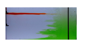
First, we illustrate the flow that occurs in steady state. In figure 1 we present a series of images showing how a pulse of dye injected into the flow evolves in time when the system is in steady state. In the case of WT, the dye is released into the interior of the tank. Panel (a) illustrates the evolution of this dye over a period of 10 min, showing both vertical and lateral mixing. Figure 1(c) shows a time series of a vertical line in the tank, converted to false colour, to illustrate how the dye spreads vertically through the tank during the experiment. This is compared with the theoretical solution (see § 4 for the model) for the position of the peak of the dye concentration as it evolves in time, which is plotted in a red dashed line. We see that the dye rises at a rate consistent with the mean upwelling rate  $\bar {w}$.

Figure 1. Illustration and quantification of the mixing of dye in the case of (a,c) WT and (b,d,e) BM, showing the differences in the mixing process. (a,b) Colour photographs of a front view of the experimental tank, showing the evolution of a patch of dye as it is mixed. Schematic summaries show (a) fluid subject to the same uniform upwelling and mixing throughout the tank; and (b) fluid upwelling and mixing only in the BM region, whose boundary is marked by vertically layered intrusion structures. (a) Photographs are shown at times of 0, 20, 60, 120, 300 and 600 s after the dye has been released. (b) Photographs show the evolution of dye (bi) at times 0, 66 and 133 min after the release of red dye and (b) 20 s and 2, 6 min after the release of green dye. (c–e) Time series of horizontally averaged sections containing dye, where dye intensity is shown in false colour and in which dye, normalised at maximum intensity to 1, is shown red–yellow–green–blue for decreasing dye concentration. Overlain is a red dashed line showing the peak of the spreading of tracer in a numerical calculation (see § 4). These panels show the horizontally averaging of dye in: (c) a 30 cm wide section on the left side of the tank showing the mixing of red dye in the case of WT, (d) a narrow section in the turbulent mixing region showing the mixing of green dye, (e) a narrow section in the middle of the tank, containing the tip of the dye at  $t = 0\,\text {min}$, showing the mixing of the red dye in the case of boundary mixing.
In the case of BM (figure 1b), a pulse of red tracer is again released into the interior of the tank. We see that this dye maintains the same vertical position and remains horizontal throughout the 190 min of the experiment (figure 1e). On the other hand, a pulse of tracer injected into the boundary region, shown in green, mixes rapidly in the vertical direction (figure 1d) as it rises through the mixing region. The left-hand interface of the turbulently mixing dye is marked by vertically layered intrusion structures which move into and out of the BM region, although a distinct interface is kept between the clear and green fluid. These intrusions grow in length over a much longer time scale than the time scale taken for the dye to mix vertically and upwell through the depth of the tank. The theoretical solution for the location of the centre of the pulse of dye, if all the fluid travels through the boundary region of length  $L_B = 30$ cm with an enhanced upwelling rate $\bar {w}({L}/{L_B})$ and diffusivity $\kappa _B = \bar {\kappa }({L}/{L_B})$, is shown for comparison (red, dashed, see § 4).
In each experiment we measure the vertical salinity profile in steady state. The normalised profiles are shown in figure 2(a) and further discussed in § 4.

Figure 2. (a) Vertical profiles of normalised buoyancy as a function of depth. The different ratios of the averaged upwelling to diffusivity  $\gamma = {\bar {w} H}/{\bar {\kappa }}$ are indicated by the colours: $\gamma = 7.1$ (blue), $\gamma = 3.4$ (red), $\gamma = 2.4$ (green) and $\gamma = 0.7$ (purple). Experimental data for both the cases of BM (dashed) and interior mixing (dotted) are compared with the predictions of the steady-state model (solid). (b) Scatter plot showing the ratio of salinity flux implied by the salinity profile as described in the text, $F_s$, plotted as a function of the experimental salinity flux. Ten experiments are shown in which the mixing scenario is either WT (red) or boundary mixing (yellow).
4. Steady-state model
In Part 1 we found that the salinity in the tank is horizontally uniform and may be described according to a one-dimensional diffusion model ((6.4), Part 1). The resulting steady vertical salinity structure in the tank was a result of the balance between the turbulent diffusive and advective fluxes at each depth in the tank.
4.1. Governing equations
We again assume that the salinity is horizontally uniform. In the case of WT, the upwelling rate is the volume flux into the bottom of the tank averaged over the cross-sectional area,  $\bar {w} = {Q_B}/{BL}$ and we assume the bulk diffusivity $\bar {\kappa }$ takes the value as measured in the previous experiments (see Part 1). In steady state, we expect a balance between the advective and diffusive fluxes so that the steady-state salinity, $\tilde {S}$, is given by
 \begin{equation} \frac{Q_B}{BL}\frac{\partial \tilde{S}}{\partial z} = \bar{\kappa} \frac{\partial^2 \tilde{S}}{{\partial z}^2}. \end{equation}
 With BM, the interior region has length  $L_I$ and is quiescent with negligible diffusivity $\kappa _I \approx 0$. The boundary region has length $L_B$ with an effective turbulent diffusivity $\kappa _B$. As demonstrated by the motion of the dye in the interior and in the boundary region (§ 3), the upwelling in the system occurs in the boundary mixing region, and so we expect $w_B = {Q_B}/{BL_B}$. The salinity in the boundary region is expected to follow the advection–diffusion balance
 \begin{equation} \frac{Q_B}{BL_B} \frac{\partial \tilde{S}}{\partial z} = \kappa_B \frac{\partial^2 \tilde{S}}{{\partial z}^2}. \end{equation}
We note that (4.1) and (4.2) are equivalent if  $\kappa _B L_B = \bar {\kappa } L$.
Equations (4.1) and (4.2) have solution for the salinity (cf. Munk Reference Munk1966)
 \begin{equation} \tilde{S}(z) = S_0' + (S_1' - S_0') \frac{ \exp\left(\dfrac{ \bar{w} (z - z_0) }{ \bar{\kappa} } \right) - 1 }{ \exp\left( \dfrac{ \bar{w}H }{ \bar{\kappa} }\right) - 1}, \end{equation}
where  $S = S_0'$ at $z=z_0$, $S = S_1'$ at $z=z_1$ and $H = z_1 - z_0$.
4.2. Comparison with experimental data
In the experiments the injection of fluid leads to additional turbulent mixing in the regions near the upper and lower boundaries of the tank, and so the effective turbulent mixing is different in detail from that produced purely by the movement of the rake.
In comparing the model salinity profiles (4.3) with the experimental data, we therefore work with the salinity data collected in the tank from a depth 5 cm above the base to a depth 5 cm below the surface (50 cm above the base). Once the system has reached steady state, the time-averaged salinity  $\bar {S}(z)$ at each depth from $z = 5$ to $z = 50$ cm is compared with (4.3) and the values $S_0'$ and $S_1'$ are systematically varied to find the minimum least squares error, defined by
 \begin{equation} \text{Error} = \sqrt{\frac{1}{n-3}\sum_{i=2}^{n-2} \left[ \frac{\bar{S}(z_i) - S_1'}{S_0' - S_1'} - \left( 1 - \frac{ \exp\left( \dfrac{ \bar{w} (z_i - z_0) }{ \bar{\kappa} } \right) - 1 }{ \exp\left(\dfrac{ \bar{w}H }{ \bar{\kappa} }\right) - 1} \right)\right]^2}, \end{equation}
where  $n$ is the total number of samples, taken at 5 cm intervals.
The experimental data are then rescaled according to the relation
 \begin{equation} s(z) = \frac{\bar{S}(z) - S_1'}{S_0' - S_1'}, \end{equation}
and this is shown in figure 2(a) as a function of depth in the tank for experiments in which  $\gamma = 7.1$ (blue), $\gamma = 3.4$ (red), $\gamma = 2.4$ (green) and $\gamma = 0.7$ (purple). We also show the theoretical best-fit Munk profiles (4.3), $\tilde {S}(z)$ for each case. In each case, these profiles have a least squares error smaller than 5 % with a mean least squares error of 3.5 %.
The best-fit profile,  $\tilde {S}$, has an associated salinity flux $F_s = Q_B\tilde {S} - \bar {\kappa } A ({\partial \tilde {S}}/{\partial z})$. In figure 2(b) we show that the salinity flux $F_s$ is very similar to the salinity flux $Q_BS_B$ which is supplied at the base of the tank, and this provides a consistency check on the model. The small difference in the salinity flux associated with the best fit empirical salinity profile and the salinity flux supplied at the base of the tank (figure 2(b)) is consistent with the small errors in the experiment associated with fluctuations in the pump flow rate with time. This is measured at various times in the experiment, and introduces an error of order 7 % over the course of the experiment, coupled with errors of 1 %–2 % using the refractometer to measure salinity.
4.3. Boundary conditions
As noted in the previous subsection, additional mixing processes occur at the top and the bottom boundaries. If we assume that the diffusivity  $\bar {\kappa }$ is constant vertically through the tank then we can apply the boundary conditions at the top and base of the tank to derive an idealised solution. In this subsection, we quantify the error between the idealised solution and the empirical salinity profiles.
At the base of the tank, the sum of the advective and diffusive fluxes within the tank,  $-\bar {\kappa } B L_B \frac {\partial S}{\partial z}(0,t) + Q_BS(0, t)$, matches the source of salinity supplied $Q_BS_B$
 \begin{equation} -\bar{\kappa} BL\frac{\partial S}{\partial z}(0,t) = Q_B(S_B - \tilde{S}(0, t)). \end{equation}
 At the surface of the tank, the advective and diffusive flux in the tank matches the flux of salinity removed from the tank,  $(Q_B + Q_T) S(H,t)$
 \begin{equation} -\bar{\kappa} BL\frac{\partial S}{\partial z}(H,t) = Q_T( \tilde{S}(H, t) - S_T). \end{equation}
 Assuming that the salinity follows the Munk profile (4.3), it follows that the values  $S_0'$ and $S_1'$ are
 \begin{equation} \begin{bmatrix} S_1' \\ S_0' \end{bmatrix}= \frac{1}{1 - (b - 1)(a - 1)} \begin{bmatrix} bS_B + (1 - b)aS_T\\ (1 - a)bS_B + aS_T \end{bmatrix}, \end{equation}
where  $\bar {w}_T = {Q_T}/{BL}$, $a = ({(1 - \exp ({\bar {w}H}/{\bar {\kappa }}))}/{\exp ({\bar {w}H}/{\bar {\kappa }})}) ({\bar {w}_T}/{\bar {w}})$ and $b = 1 - \exp ({\bar {w}H}/{\bar {\kappa }})$. For completeness, we have included $S_T$, the salinity of the injected fluid, but this is normally fresh water.
When we compare these theoretical salinity profiles with the experimental salinity profiles from  $z = 5$ to $z = 45$ cm, the root-mean-square error is less than 10 % for each value of $\gamma$, where the least squares error is defined by
 \begin{equation} \text{Error} = \frac{\sqrt{\dfrac{1}{n-3}\displaystyle\sum_{i=2}^{n-2} (\bar{S}(z_i) - \tilde{S}(z_i))^2}}{\dfrac{1}{n-3}\displaystyle\sum_{i=2}^{n-2} \bar{S}(z_i)}, \end{equation}
where  $n$ is the total number of samples of the vertical salinity profile.
In later sections of this paper we focus on the flow that develops when the buoyancy fluxes supplied to the system are changed. When modelling these flows, we continue with these idealised boundary conditions (4.6) and (4.7) assuming that the diffusivity is a constant, and noting that an error of up to 10 % in the salinity profiles may arise as a result.
4.4. Dye evolution
In the case of WT, we hypothesise that dye released into the tank with concentration  $C$ evolves according to the diffusion equation with the same diffusivity, $\bar {\kappa }$, and upwelling, $\bar {w}$,
 \begin{equation} \frac{\partial C}{\partial t} + \bar{w} \frac{\partial C}{\partial z} = \bar{\kappa} \frac{\partial^2 C}{{\partial z}^2}. \end{equation}
At the base of the tank, there is no supply of dye into the tank
 \begin{equation} -\bar{\kappa} B L\frac{\partial C}{\partial z}(0,t) + Q_B C(0, t) = 0. \end{equation}
At the surface of the tank, the advective and diffusive flux in the tank matches the removal of dye from the tank at a rate,  $(Q_B + Q_T) C(H,t)$
 \begin{equation} -\bar{\kappa} B L\frac{\partial C}{\partial z}(H,t) = Q_TC(H, t). \end{equation}
We have solved this equation with the above boundary conditions to explore the mixing and the motion of a pulse of dye injected into the tank. We assume for simplicity that the diffusion is constant throughout the depth of the tank. The position of the centre of mass of the dye pulse is shown in figures 1(c) and 1(d) for the case of full interior mixing (figure 1c) and BM, where the pulse of dye is released in the BM region (figure 1d). It is seen that the model is in reasonable agreement with the experimental data for the location of the centre of the dye pulse as a function of time. In each case, we use the value for the diffusivity obtained from Part 1.
5. Increase in buoyancy: experimental observations
We present the data and observations for the transient experiments in which there is a net gain in the total buoyancy in the system. Starting with a tank filled with fresh water, fluid of constant salinity  $S_B = S_0$ is injected into the bottom of the tank at a constant flow rate $Q_B$, which leads to a continuous increase in the salinity of the system until the stratification reaches a steady-state distribution. We describe two experiments in which the mixing occurs either across the entirety of the tank or in which the mixing is confined to one region of the tank. In both experiments, fluid is injected at a rate of $5.6\ \text {cm}^3\ \text {s}^{-1}$, and ventilates the volume of the tank over a time scale of ${AH}/{Q_B} \approx 3.5\ \text {h}$. The salinity injected at the base of the system is transported through the tank by a combination of advective and diffusive fluxes, and the ratio of these fluxes is described by the non-dimensional number $\gamma = {\bar {w}H}/{\kappa }$. In the experiment with BM (experiment 11), $\gamma = 2.9$ and in the case of WT (experiment 12), $\gamma = 4.3$.
In figure 3 we show a series of salinity profiles at various intervals throughout the duration of the experiments as the system transitions towards steady state, for experiments (a) 11 and (b) 12 with (a) BM and (b) WT. In both cases, the system reaches steady state after approximately 7 hours. In comparing the two experiments, the diffusive component of the transport is larger in the experiment with BM. We see in (a) that as the system gains salinity over time, the profiles remain approximately linear and the resulting steady-state salinity profile has a more linear shape. In the experiment with WT, the salinity gain in the system at first remains concentrated in the lower depths of the tank, and reaches the upper depths of the tank only towards the later stages in the transition to steady state. The salinity profile in the tank has a lower 30 cm layer of almost constant salinity above which there is a surface layer with a sharp salinity gradient.

Figure 3. Salinity profiles in time from the experiments with an increase of salinity in the system in the case of (a) BM (experiment 11) and (b) WT (experiment 12). Salinity profiles are chronologically ordered in colour (blue, red, purple) and are textured within each colour (solid cross, solid circle, dashed cross, dashed circle).
5.1. Boundary mixing case
In the case of BM, we release two lines of red and green dye at heights 45 and  $25\ \text {cm}$ respectively into the tank interior to image the flow. The stratification evolves for 90 min before the dye is added so that there is some stratification throughout the tank. In figure 4(a-ii)–(a-vi) we display a series of photographs showing the evolution of the dye as the experiment progresses. We see that the dye in the tank interior does not undergo mixing and also that the upwelling in the tank is horizontally uniform as the lines of dye remain horizontal. From its release at $t = 90\,\text {min}$, the red dye upwells in the tank interior and reaches the surface of the system over the first twenty minutes. At the surface of the fluid, there is a strong horizontal current in which the red dye is transported from the interior to the BM region. In the boundary region, the red dye can be seen to mix vertically across the height of the tank, and some of the red fluid detrains from this region at all heights. The green line of dye is released 25 cm above the base and then upwells from its depth of release to the surface of the tank in a similar fashion to the red dye, with the travel occurring over a duration of 75 min. The horizontal line of green dye can be seen to first contract and later expand in the horizontal direction as it upwells, which can be seen in (a-ii)–(a-v).

Figure 4. Overview of the experimental observations in the case in which the buoyancy in the system increases, in the case of (a) BM, experiment 11, and (b) WT, experiment 12. The times displayed are as measured from the beginning of the experiment when initially filled with fresh water. (i) Schematics of the flow dynamics. (a-ii)–(a-vi) True-colour photographs of the experimental domain at times  $t = (a\text {-ii})\ 90$, $(a\text {-iii})\ 110$, $(a\text {-iv})\ 150$, $(a\text {-v})\ 165$, $(a\text {-vi}) 190\,\text {min}$. (a-vii) True-colour time series of a vertical line within the interior, containing the lines of red and green dye, overlain with the experimental isopycnals. (b-ii)–(b-vi) Dye concentration, represented in false colour, of the experimental domain at times $t = (b\text {-ii})\ 140$, $(b\text {-iii})\ 142$, $(b\text {-iv})\ 155$, $(b\text {-v})\ 170$, $(b\text {-vi})\ 200\,\text {min}$. The location of the mixing rake can be seen in the images as a vertical red bar and its position from image subtraction can be seen as a vertical blue bar. (b-vii) False-colour time series of the horizontally averaged dye concentration over the left-hand section of the tank containing the line of dye. Overlain is a red dashed line showing the peak of the spreading of tracer in a numerical calculation.
In panel (a-vii) we present a time series of a vertical line containing the red and green dyes over time and overlay it with the isopycnals from the salinity profiles presented in figure 3. The rise of the lines of both the red and green dyes closely follows the rise of their adjacent isopycnals. Over the first 100 min of the dye study, the isopycnals rise in height at a rate approximately independent of height, and we note that there remains a distinct boundary between the dyed fluid and its surrounding clear fluid. We infer from this that the changing stratification drives the advection of interior fluid so that that the parcels of fluid remain neutrally buoyant, and entrainment and detrainment occur to conserve volume with respect to this depth-varying process. It is important to note that this process occurs with a net transport of volume from the base of the tank to the surface. The flow dynamics is summarised schematically in (a-i).
5.2. Whole-tank mixing case
In figure 4(b-ii)–(b-vi) we present a similar dye study for the case of WT in which a line of dye is released at a height of 25 cm to showcase the flow. Over the first 30 min of the study, the dye can be seen to mix both laterally and vertically.
In (b-vii) we present the time series of a horizontally averaged vertical section of the tank, of width spanning approximately 80 cm from the left-hand portion of the tank, showing the spatial evolution of the dye. This is compared with the numerically calculated solution (the model used was introduced in § 4.4), where the initial distribution of the dye is approximated by a Gaussian curve with best-fit values for its centre of mass and width. The height of maximum concentration of this solution is overlain on top of the time series in a red, dashed line, and we see that this numerical model with a diffusive flux with constant diffusivity  $\bar {\kappa } = 0.06\ \text {cm}^2\ \text {s}^{-1}$ is consistent with the experimental evolution of the dye. It can be noted that the background density stratification evolves significantly over the two hour period, yet the mixing of the dye that occurs remains consistent with a diffusive model with constant diffusivity.
6. Increase in buoyancy: model
In this section we apply the theoretical model presented in § 4 to the experiments described in § 5 to investigate the motion of interior dyed fluid as well as the changing stratification. We saw that, with a changing stratification in the case of BM, the interior fluid parcels sink or rise at the same rate as the isopycnals, giving rise to a velocity perturbation in the interior and a counter-flow in the BM region.
6.1. Governing equations
We modify the model to include the time-dependent terms. In the case of WT, using the values for the upwelling rate  $\bar {w}$ and diffusivity $\bar {\kappa }$, we expect the salinity $S(z,t)$ to evolve according to the advection–diffusion equation
 \begin{equation} \frac{\partial S}{\partial t} + \frac{Q_B}{BL}\frac{\partial S}{\partial z} = \bar{\kappa} \frac{\partial^2 S}{{\partial z}^2}. \end{equation}
 As shown earlier in § 3, in steady state and in the case of BM, there is a constant net upwelling rate  ${Q_B}/{BL_B}$ that occurs primarily through the boundary region in our experiments. The contribution of mixing from the mechanical stirring in the boundary region dominates that from the molecular diffusivity in the interior region. We therefore expect that any transient evolution of the density field associated with changes in the buoyancy flux will be affected by an additional flow in the BM region with an equal and opposite flow in the interior. We denote this additional transient flow by $W_I$ and $W_B$ in the interior and boundary regions, respectively, with no net additional flow, as given by
 \begin{equation} W_IL_I + W_BL_B = 0. \end{equation}
The convergence of this flow drives intrusions from the boundary region into the interior, as given by
 \begin{equation} \frac{\partial}{\partial z} (W_BL_B) =-U =- \frac{\partial}{\partial z} (W_IL_I), \end{equation}
where  $U$ is the lateral flow from the boundary region into the interior.
We continue by considering the flux balance on a fluid slice in the boundary region where the salinity  $S_B$ is described by
 \begin{equation} \frac{\partial}{\partial t}(L_B S_B) + \frac{\partial}{\partial z}\left(\frac{Q_B}{B}S_B + W_B L_B S \right) - \frac{\partial}{\partial z} \left( L_B \kappa_B \frac{\partial S_B}{\partial z} \right) =-US_B,\quad L_I \leq x \leq L_I + L_B. \end{equation}
Combining this with (6.3) leads to the result
 \begin{equation} \frac{\partial S_B}{\partial t} + \left( \frac{Q_B}{BL_B} + W_B(z,t) \right)\frac{\partial S_B}{\partial z} = \kappa_B \frac{\partial^2 S_B}{{\partial z}^2},\quad L_{I} \leq x \leq L_{I} + L_{B}. \end{equation}
The same approach for the interior with negligible diffusivity leads to a similar result
 \begin{equation} \frac{\partial S_I}{\partial t} + W_{I}(z,t)\frac{\partial S_I}{\partial z} = 0,\quad x \leq L_{I}. \end{equation}
 The salinity is assumed to remain uniform horizontally  $S_I = S_B = S(z, t)$ with the exception of boundary layers which form at the surface and basal boundaries, where fluid transfer is strongly influenced by horizontal advective fluxes. By considering a fluid slice across the domain, the net advective flux has an average upwelling rate $\bar {w} = {Q}/{BL}$, and by adding (6.5) multiplied by the length $L_B$ and its complement (6.6) multiplied by $L_I$, we find that salinity in the tank evolves according to
 \begin{equation} \frac{\partial S}{\partial t} + \frac{Q_B}{B(L_I + L_B)}\frac{\partial S}{\partial z} = \frac{\kappa_B L_{B}}{L_I + L_B} \frac{\partial^2 S}{{\partial z}^2}, \end{equation}
with tank-averaged diffusivity  $\bar {\kappa } = {\kappa L_B}/{(L_I + L_B)}$.
The boundary conditions we use are as described in § 4.3.
Equation (6.6) suggests that the interior vertical velocity perturbation
 \begin{equation} W_I =-\frac{\displaystyle\dfrac{\partial S}{\partial t}}{\displaystyle\dfrac{\partial S}{\partial z}},\end{equation}
is a result of interior fluid parcels following the changing isopycnals.
We now compare the predictions of this model with experimental data relating to both the evolution of the salinity and also the migration of fluid surfaces in the case that a steady buoyancy flux is supplied to the base of an initially uniform layer of fluid. As seen in § 4, in this experiment, the system eventually converges to a steady state, which is described by the Munk solution.
6.2. Boundary mixing flow predictions
In the BM experiments presented in § 5, we saw that the dyed fluid in the interior of the tank upwelled at the same rate as the isopycnals, along with a horizontal compression of the fluid parcels. In figure 5(a) we present the time series (originally shown in figure 4(a-vii)) of a vertical line within the interior, showing the depths of the dye as a function of time. We then plot the isopycnals found from the numerical solution of the model presented in the previous subsection as a function of time. As may be seen in figure 5, the ascent of the isopycnals mirrors the migration of the dye.

Figure 5. (a) Time series of a vertical line, during experiment 11, within the interior showing the vertical depths of the red and green lines of dye as a function of time (repeated from figure 4a-vii) overlain with isopycnals from the analytical model. (b) Collage of the green lines of dye taken from images at the times  $t = 90, 110, 130, 150, 165\,\text {min}$, overlain onto the image from $t = 90\,\text {min}$. Overlain (white) is the prediction of the particle path, with the initial position taken to be the tip of the green dye at $t = 90\,\text {min}$.
The rise of the lines of the dye suggests that the upwelling speed within the interior of the tank remains horizontally uniform. By local mass conservation, the lateral speed
 \begin{equation} U_I =-\frac{\partial W_I}{\partial z} (x - x_0), \end{equation}
where  $U_I = 0$ on the left boundary, $x = x_0$, and the particle path with initial position $\boldsymbol {x_0}$ at time $t$ may be predicted by
 \begin{equation} \boldsymbol{x}(t) = \boldsymbol{x}_0 + \int_0^t\boldsymbol{u}_I(\boldsymbol{x}(t), t)\,{\rm d}{t}. \end{equation}
 In figure 5(b) we present a collage of the green lines of dye, taken from images at the times  $t = 90, 110, 130, 150, 165\,\text {min}$, overlain onto the image at $t = 90\,\text {min}$. Overlain onto this collage, in white, is the particle path taken from integrating (6.10). The model appears to provide a reasonable representation of the observations, predicting the initial lateral leftward movement of the dye, as well as the eventual rightward movement.
6.3. Comparison of salinity profiles
In figure 6 we compare the experimental measurements of the salinity with the theoretical solution in the case of BM (experiment 11, (a)) at the times  $t =$ (blue) $30$, (red) $120$, (magenta) $180$, (green) 450 min and in the case of WT (experiment 12, panel b) at times $t =$ (blue) $50$, (red) $135$, (magenta) $280$, (green) 400 min. The least squares error between the theoretical and measured salinity profiles remains below 10 % in the case of WT and below 8 % in the case of BM and this is consistent with the error between the empirical and model steady-state solutions presented in § 4 assuming the diffusivity is constant over the whole depth of the tank.

Figure 6. (a) Comparison of the (dashed) theoretical and (solid) experimental salinity profiles in the case of (a) BM and (b) WT. The salinity profiles are shown at times (a)  $t =$ (blue) $30$, (red) $120$, (magenta) $180$, (green) 450 min and (b) $t =$ (blue) $50$, (red) $135$, (magenta) $280$, (green) 400 min.
7. Decrease in buoyancy: experimental observations
In § 5, the experiments started from an initially fresh system and saline water was injected into the bottom of the tank, leading to an increase in the buoyancy of the system with time. In this section, we present two experiments in which there is a gradual decrease in the buoyancy flux supplied to the system and again compare the two cases in which the tank has local mixing or is uniformly mixed throughout.
The stratification initially follows the steady Munk profile, where the fluid is pumped into the base of the tank at rate  $Q_B$ with salinity $S_B = S_0$ and fresh water with salinity $S_T = 0$ is pumped into the top of the tank at a rate $Q_T$, and fluid is extracted from the surface of the tank at rate $Q_B + Q_T$. The salinity of the injected fluid then decreases slowly and linearly in time as previously given by (2.1)
 \begin{equation} S_B(t) = S_0 \left(1 - \varDelta \frac{t}{T}\right)\!, \end{equation}
where the values  $\varDelta$ and $T$ are those described in table 1.
In figure 7 we plot the salinity profiles taken at intervals throughout the duration of the experiment. In both experiments, as time progresses, the salinity of the injected fluid is reduced to below that of the salinity at the base of the tank. This leads to an additional effect where the injected fluid becomes unstable on injection into the tank and we find a well-mixed layer forming at the bottom of the system with a depth that grows in time.

Figure 7. Salinity profiles in time from the experiments with a net decrease of salinity in the system in the case of (a) BM (experiment 13) and (b) WT (experiment 14). Salinity profiles are chronologically ordered by colour (blue, red, purple, grey) and are textured within each colour (solid cross, solid circle, dashed cross, dashed circle).
7.1. Boundary mixing case
When the mixing occurs through BM, the values used are  $\varDelta = 0.29$ and $T = 390\,\text {min}$. Two lines of red and green are dyes are injected into interior of the tank at time $t = 0\,\text {min}$. In figure 8 we illustrate the flow that occurs over the duration of the experiment by showing a series of images of the tank detailing the evolution of the two lines of dye (red and green) in the interior fluid.

Figure 8. Overview of the experimental observations in the case of BM and when the net buoyancy decreases. Displayed times are measured from the beginning of the experiment when the ramp down of injected salinity occurs. (a-i) Schematic of the flow dynamics. (a-ii)–(a-x) True-colour photographs of the experimental domain at times  $t = (a\text {-ii})\ 0$, $(a\text {-iii})\ 73$, $(a\text {-iv})\ 123$, $(a\text {-v})\ 151$, $(a\text {-vi})\ 171$, $(a\text {-vii})\ 218$, $(a\text {-vii})\ 332$, $(a\text {-ix})\ 377$, $(a\text {-vi})\ 405\,\text {min}$. (b) True-colour time series of a vertical line within the interior, containing the lines of red and green dye, overlain with the experimental isopycnals.
For the first 70 min of the experiment, we see that the lines of dye remain at approximately the same vertical height. We also see some horizontal spreading, where the red dye appears to spread out laterally whilst the green dye contracts. The green dye downwells over the next 100 min, slowly at first and gradually faster once the green dye approaches the bottom of the tank. While the green dye downwells, it can be seen to contract horizontally towards the left side of the tank and the axis through the dye seems to remain horizontal. Throughout this process the dye does not appear to mix and maintains an interface with the clear fluid. Once the green dye approaches the bottom of the tank, intrusion structures begin to appear within the green dye. This can be seen more clearly at  $t = 171$ min, at which point the green dye travels quickly along the bottom of the tank, is mixed up in the turbulent mixing region and intrudes back into the tank. Over this duration the red dye moves approximately three centimetres vertically downwards. From $t = 171$ to $t = 405\,\text {min}$, the red dye downwells in a similar fashion to the green dye by downwelling and shortening in the horizontal direction. Furthermore, horizontal gradients in the dye concentration begin to form within the intruded green dye over the period of time $218\,\text {min} < t < 377\,\text {min}$, suggesting that the regions closer to the mixing grid have a quicker ventilation time than the dye in the interior.
In figure 8 we present a time series of a vertical line within the interior, showing the depths of the dye as a function of time. We then overlay the isopycnals from the experimental salinity profiles on top. The lines of dye follow the isopycnals, suggesting that, in this case, interior parcels of fluid sink in line with falling isopycnals to remain neutrally buoyant, in a similar fashion to the experiments presented in §§ 5 and 6.
7.2. Whole-tank mixing case
When the mixing occurs through whole tank mixing, the experimental parameters in (2.1) are  $\varDelta = 0.32$ and $T = 405\,\text {min}$. At time $t = 165\,\text {min}$ a line of red dye is injected into the interior of the tank at an approximate depth of $z = 28$ cm. At this time, the fluid is buoyant upon injection and undergoes unstable convection. In figure 9(a), we plot a series of images showing the mixing of the dye from the time it is injected until $t = 190\,\text {min}$. The dye mixes laterally and vertically for the first 3 min. At $t = 175\,\text {min}$, we see that the portion of dye towards the middle of the tank upwells while the dye on the left-hand side of the tank appears to have downwelled slightly. This flow pattern continues past $t = 180\,\text {min}$ and, at $t = 190\,\text {min}$, we can see that a portion of dye has sunk into the bottom-left corner of the tank while the rest of the dye is approximately horizontally uniform and has upwelled in the tank interior. In figure 9(b) we show a time series of a vertical line in the tank showing the mixing of the dye. In (b-i) this vertical line is taken in the left portion of the dye patch, and here the dye appears to be slowly downwelling as the experiment progresses. In (b-ii) we repeat this for the dye in the middle of the dye patch and here the dye upwells as the experiment progresses, consistent with the mean rate $\bar {w}$.

Figure 9. Overview of the experimental observations in the case of WT and when the net buoyancy decreases. (a-i)–(a-v) True-colour photographs of the experimental domain at times  $t = (a\text {-i})\ 165$, $(a\text {-ii})\ 168$, $(a\text {-iii})\ 175$, $(a\text {-iv})\ 180$, $(a\text {-v})\ 190$. (b) False-colour time series of a vertical line on the (i) left side and (ii) middle of the dye patch, showing the mixing of the dye. In (b-ii) the peak of the numerically calculated evolution of a Gaussian is overlain (red, dashed) onto the time series.
8. Decrease in buoyancy: model
In § 7, we saw that in the case that the buoyancy decreases, interior fluid downwells.
We found that, once the salinity of the injected fluid into the base of the tank reduces below that of the fluid at the base of the tank, unstable convection develops following injection. When this occurs, a well-mixed layer of height  $h_m(t)$ forms at the base of the tank with salinity $S = S(h_m,t)$. As time progresses, the depth of this layer grows due to the net loss of salinity in the system.
To account for this additional process of mixing, we adapt the model of § 6. When the salinity of the input fluid  $S_B(t)$ decreases to below that of the salinity at the base of the tank, $S_B(t) < S(0,t)$, we change the boundary condition at the base of the tank to
 \begin{equation} \frac{\partial S}{\partial z}(0,t) = 0. \end{equation}
We account for the subsequent growth of the well-mixed layer  $h_m$ according to the relation
 \begin{equation} \frac{\partial [h_mS(h_m,t)]}{\partial t} = \bar{w}(S_B - S(h_m, t)). \end{equation}
8.1. Boundary mixing flow predictions
In figure 10(a) we present the time series (originally shown in figure 8b) of a vertical line within the interior, showing the depths of the dye as a function of time. However, now we also plot the isopycnals found from the theoretical model as a function of time and find that these mirror the vertical rise of the dye lines. In § 6.2 we calculated the interior velocity, given by (6.8), and used local mass conservation to calculate the lateral velocity. The particle path can be integrated, as given by (6.10), where we use  $x_0 = 2$ cm in (6.9). In figure 10(b) we take a series of images from experiment 14 at given intervals and collage the lines of green dye onto a single image. Starting with the initial position of the tip of the lower portion of the green dye at $t = 0$ min, the particle path is then overlain on top of the collage in white. Our model prediction of the flow is consistent with the lateral compression of the green dye as it downwells towards the corner.

Figure 10. (a) Time series of a vertical line, during experiment 13, within the interior showing the vertical depths of the red and green lines of dye as a function of time (repeated from figure 8b) overlain with isopycnals from the numerical model. (b) Collage of the green lines of dye taken from images at the times  $t = 0, 73, 123, 151\,\text {min}$, overlain onto the image from $t = 0\,\text {min}$. Overlain (white) is the prediction of the particle path, with the initial position taken to be the tip of the green dye at $t = 0\,\text {min}$.
8.2. Comparison of salinity profiles
We compare the experimental salinity profiles and the theoretical solution in the case of BM in figure 11(a) and in the case of WT in figure 11(b). The error in both cases remains approximately constant at 5 % in the case of BM and 3 % in the case of WT. This provides support for the theoretical picture we have developed of the flow and evolution of the salinity associated with the transient BM.

Figure 11. Comparison of the experimental (solid) and theoretical (dashed) salinity profiles in the case of (a, experiment 13) at the times  $t =$ (blue) $0$, (red) $135$, (magenta) $285$, (green) 405 min and in the case of BM (b, experiment 14) at the times $t =$ (blue) $0$, (red) $160$, (magenta) $270$, (green) 390 min.
9. Discussion
In this paper we have investigated the interaction of a mean upwelling through a closed basin with a vertical buoyancy flux, in two cases in which the fluid is either mixed at the same rate across the basin by a rake which oscillates across the whole basin, representing the WT regime, or by a rake which oscillates near one vertical boundary, leading to the BM regime.
In steady state, we found that, in the case with WT, upwelling and vertical mixing occurred at the same rate throughout the tank. In the case of BM, the upwelling and turbulent diffusive buoyancy transport are primarily confined to the BM region. We presented a series of experiments systematically varying the bulk upwelling and the bulk diffusivity and found that the steady vertical salinity structure is independent of the type of mixing, whether it is distributed across the tank or confined to one portion of the tank. The stratification is set by an intricate balance between the upward advection of salinity balancing the loss of salinity through diffusive mixing such that the total flux of salinity is conserved at each depth in the tank, and this is determined by the ratio of the bulk upwelling,  $\bar {w}$, to the bulk diffusive flux, ${\bar {\kappa }}/{H}$, forming the non-dimensional number ${\bar {w}H}/{\bar {\kappa }}$. In more general situations in which the turbulent mixing varies horizontally in space across a basin, then for the isopycnals to remain horizontal, the local balance between the vertical advection and diffusion of salinity must match the same balance satisfied by the bulk properties. This implies that the local upwelling rate $w_i$, in regions $i$ with length $L_i$ and diffusivity $\kappa _i$, where regions have constant width, satisfies the relation
 \begin{equation} \frac{w_i}{\kappa_i} = \frac{\bar{w}}{\bar{\kappa}}, \end{equation}
where the bulk upwelling rate is the mean of the upwelling in the different regions
 \begin{equation} \bar{w} = \frac{Q_B}{A} = \frac{\displaystyle\sum_i w_i L_i}{\displaystyle\sum_i L_i}, \end{equation}
and the bulk diffusivity is the mean of the diffusivity in the different regions
 \begin{equation} \bar{\kappa} = \frac{\displaystyle\sum_i \kappa_i L_i}{\displaystyle\sum_i L_i}, \end{equation}
such that these bulk parameters describe the advective and diffusive transport across the whole system.
We presented an extension to the analytical model first presented in Part 1 (Li & Woods Reference Li and Woods2023) that describes the dynamics in systems with a changing stratification where, in the case of boundary mixing, the tank is partitioned into two regions where one region contains diffusive mixing and where the second region has no mixing. This was able to accurately predict the vertical and horizontal flow that developed in the interior region of the tank. It was also able to predict the evolution of the salinity with reasonable accuracy, noting the model simplification that the turbulent diffusivity is constant through the vertical depth of the tank and to the boundaries.
Our experiments of the transient mixing also suggest that this distribution of upwelling persists when the salinity fluxes supplied at the vertical boundaries of the system change, although with additional transient flows that are a result of the changing stratification. In the case of BM, a change in the forcing buoyancy fluxes leads to a change in the buoyancy stratification of the fluid in the BM zone such that the diffusive flux is divergent; in turn this drives an additional flow in the boundary region such that the advective flux balances the divergence of the diffusive flux. By mass conservation, this drives an equal and opposite flow in the interior. We show that the interior fluid can either upwell or downwell, either of which occurs in the presence of a net upwelling through the system, and that the flow of fluid in the interior is instead dependent on the changes that are occurring to the stratification. In the case of an increase in buoyancy of the system, interior fluid becomes buoyant over time and upwells through the domain, consistent with the net ventilation. In the case of a decrease in buoyancy of the system, interior fluid loses buoyancy and instead downwells, opposing the direction of net ventilation in a manner consistent with the picture described by Ferrari et al. (Reference Ferrari, Mashayek, McDougall, Nikurashin and Campin2016).
The processes described in this paper provide new insight into stratified mixing in a closed and ventilated basin, especially when the mixing intensity is not uniform in space. A key learning is that the local upwelling is correlated to the local vertical diffusivity in both steady and transitioning systems: the isopycnals in our experiment are horizontal, and the local upwelling and diffusive mixing that we have investigated may be interpreted as the diapycnal velocity and diapycnal diffusion. This result may be crucial for informing field experiments using a tracer to determine ocean scale mixing; our results suggest that the advective and diffusive flux of tracer across isopycnals depends critically on its location. In addition, our experiments have identified that local regions of intense mixing may dominate the overall vertical transport of buoyancy, and the horizontal continuity of isopycnals leads to the density gradient produced in these regions being mirrored elsewhere, even though the mixing is weaker in those regions. This result illustrates the importance of quantifying local variations in the mixing intensity in terms of assessing the mean and variance of the residence time of water, and its associated properties such as dissolved CO2 content, as the water passes through the deep overturning circulation.
Declaration of interests
The authors report no conflict of interest.


 Open access