


1. Introduction
We investigate solid particle suspension, where flow advects particles and vortices shedding from particles can change surrounding flow. Such fluid–particle interactions play essential roles in many flow systems. In particular, the enhancement and attenuation of turbulence by the addition of solid particles are important in industrial and environmental flows. However, there remain many unsolved scientific issues on the complex phenomena. In fact, although turbulence modulation due to solid particles is a classical issue in fluid mechanics back to the seminal experiments by Tsuji & Morikawa (Reference Tsuji and Morikawa1982) and Tsuji, Morikawa & Shiomi (Reference Tsuji, Morikawa and Shiomi1984) about 40 years ago, there is no clear conclusion even for the most fundamental question: i.e. what determines the condition for the turbulence modulation? Gore & Crowe (Reference Gore and Crowe1989) proposed a criterion on this issue by compiling data for particulate turbulent pipe flow and a jet. They concluded that turbulence was enhanced (or attenuated) if the ratio  $D/L$, with $D$ and $L$ being the particle diameter and the integral length ( $L=0.2\times \text {(pipe radius)}$ for pipe flow, and $L=0.039\times \text {(distance from the exit)}$ for a jet), is larger (or smaller) than $0.1$ because larger particles produce turbulence in their wake, while smaller ones acquire their energy from large-scale vortices. Since then, even recently experiments with newer techniques such as particle tracking (Cisse et al. Reference Cisse, Saw, Gibert, Bodenschatz and Bec2015) and particle image velocimetry (Hoque et al. Reference Hoque, Mitra, Sathe, Joshi and Evans2016) were conducted. However, the Gore & Crowe (Reference Gore and Crowe1989) picture still holds, although Hoque et al. (Reference Hoque, Mitra, Sathe, Joshi and Evans2016), for example, proposed a more accurate estimation of the criterion of the enhancement and attenuation of homogeneous turbulence.
Numerical simulations have been playing important roles in the investigation of this complex phenomenon with many control parameters. Elghobashi & Truesdell (Reference Elghobashi and Truesdell1993) and Elghobashi (Reference Elghobashi1994) conducted numerical simulations of particulate turbulence. Their simulations were conducted with pointwise particles that obey the Maxey & Riley (Reference Maxey and Riley1983) equation, and they showed the importance of the normalized particle velocity relaxation time (i.e. the Stokes number). Although continuum approaches (Crowe, Troutt & Chung Reference Crowe, Troutt and Chung1996) were also used, we have to resolve flow around each particle to treat fluid–particle interactions accurately. Numerical methods for such direct numerical simulations (DNS) with finite-size particles were proposed in this century (Kajishima et al. Reference Kajishima, Takiguch, Hamasaki and Miyake2001; ten Cate et al. Reference ten Cate, Derksen, Portela and Akker2004; Burton & Eaton Reference Burton and Eaton2005; Uhlmann Reference Uhlmann2005). For example, Kajishima et al. (Reference Kajishima, Takiguch, Hamasaki and Miyake2001) demonstrated numerically turbulence enhancement by finite-size particles. Since then, numerical schemes (Maxey Reference Maxey2017) have been developing to more easily and accurately treat the no-slip boundary condition on particles’ surface. Thanks to these developments, many authors recently conducted DNS of particulate turbulence under realistic boundary conditions: for example, channel flow (Uhlmann Reference Uhlmann2008; Shao, Wu & Yu Reference Shao, Wu and Yu2012; Picano, Breugem & Brandt Reference Picano, Breugem and Brandt2015; Costa et al. Reference Costa, Picano, Brandt and Breugem2016, Reference Costa, Picano, Brandt and Breugem2018; Fornari et al. Reference Fornari, Formenti, Picano and Brandt2016; Wang et al. Reference Wang, Peng, Guo and Yu2016; Peng, Ayala & Wang Reference Peng, Ayala and Wang2019), pipe flow (Peng & Wang Reference Peng and Wang2019), duct flow (Lin et al. Reference Lin, Yu, Shao and Wang2017) and Couette flow (Wang, Abbas & Climent Reference Wang, Abbas and Climent2017).
In the present study, as a first step towards the complete clarification, prediction and control of the interaction between solid particles and turbulence, we examine the simplest case: namely, the modulation of turbulence by finite-size solid spherical particles in a periodic cube. Many authors (ten Cate et al. Reference ten Cate, Derksen, Portela and Akker2004; Homann & Bec Reference Homann and Bec2010; Lucci, Ferrante & Elghobashi Reference Lucci, Ferrante and Elghobashi2010, Reference Lucci, Ferrante and Elghobashi2011; Yeo et al. Reference Yeo, Dong, Climent and Maxey2010; Gao, Li & Wang Reference Gao, Li and Wang2013; Wang et al. Reference Wang, Ayala, Gao, Andersen and Mathews2014; Schneiders, Meinke & Schröder Reference Schneiders, Meinke and Schröder2017; Uhlmann & Chouippe Reference Uhlmann and Chouippe2017) studied numerically behaviours of finite-size particles in periodic turbulence. Concerning turbulent modulation, ten Cate et al. (Reference ten Cate, Derksen, Portela and Akker2004) conducted DNS of forced turbulence of particle suspension to demonstrate the enhancement of energy dissipation due to the excitation of particle-size flow. In particular, they showed that the energy spectrum was enhanced for wavenumber  $k$ larger than the pivot wavenumber $k_p\approx 0.72k_d$, with $k_d=2{\rm \pi} /D$ being the wavenumber corresponding to the particle diameter $D$, whereas it was attenuated for $k< k_p$. Similar modulation of the energy spectrum was also observed by Yeo et al. (Reference Yeo, Dong, Climent and Maxey2010), Gao et al. (Reference Gao, Li and Wang2013) and Wang et al. (Reference Wang, Ayala, Gao, Andersen and Mathews2014). An important observation in these studies is that the pivot wavenumber $k_p$ is approximately proportional to $k_d$ in forced turbulence (ten Cate et al. Reference ten Cate, Derksen, Portela and Akker2004; Yeo et al. Reference Yeo, Dong, Climent and Maxey2010), though $k_d/k_p$ varies in decaying turbulence (Gao et al. Reference Gao, Li and Wang2013). The importance of particle size was also emphasized by Lucci et al. (Reference Lucci, Ferrante and Elghobashi2010, Reference Lucci, Ferrante and Elghobashi2011). More concretely, Lucci et al. (Reference Lucci, Ferrante and Elghobashi2011) demonstrated numerically that the decay rate of turbulence depended on the particle size even if the Stokes number was identical. Gao et al. (Reference Gao, Li and Wang2013) demonstrated similar results, although they also emphasized the impact of the Stokes number on the turbulence modulation. Recall that once we fix the flow conditions, turbulence modulation can depend on, in addition to the number of particles, both the particle size and the Stokes number. Although the importance of the particle size is evident, the role of the Stokes number is still ambiguous. In particular, the condition for the turbulence modulation (i.e. attenuation or enhancement) has not been described explicitly in terms of these particle properties because of the lack of systematic parametric studies. Besides, it is also desirable to predict the degree of turbulence modulation under given flow conditions and particle properties.
The present study aims at showing the condition for finite-size particles to attenuate turbulence in a periodic cube. To this end, we conduct a systematic parametric study by means of DNS of forced turbulence, and investigate turbulence modulation due to spherical solid particles with different diameters and Stokes numbers for a fixed volume fraction. Then, based on the obtained numerical results, we propose formulae that give the condition and degree of turbulence attenuation.
2. Direct numerical simulations
2.1. Numerical methods
The fluid velocity  $\boldsymbol {u}(\boldsymbol {x},t)$ at position $\boldsymbol {x}$ and time $t$ is governed by the Navier–Stokes equation
 \begin{equation} \frac{\partial \boldsymbol{u}}{\partial t}+\boldsymbol{u}\boldsymbol{\cdot}\boldsymbol{\nabla}\boldsymbol{u} ={-}\frac{1}{\rho_f}\,\boldsymbol{\nabla}p+\nu\,\nabla^{2}\boldsymbol{u}+\boldsymbol{f}+\boldsymbol{f}^{\leftarrow p} \end{equation}
and the continuity equation
 \begin{equation} \boldsymbol{\nabla}\boldsymbol{\cdot}\boldsymbol{u}=0, \end{equation}
for an incompressible fluid in a periodic cube with side  $L_0$ ( $=2{\rm \pi}$). Here, $p(\boldsymbol {x},t)$ is the pressure field, and $\rho _f$ and $\nu$ denote the fluid mass density and kinematic viscosity, respectively. In (2.1), $\boldsymbol {f}^{\leftarrow p}(\boldsymbol {x},t)$ is the force due to suspended solid spherical particles, whereas $\boldsymbol {f}(\boldsymbol {x},t)$ is an external body force driving turbulence. In the present study, we examine the two cases with different kinds of external force $\boldsymbol {f}(\boldsymbol {x},t)$. One is a time-independent forcing (Goto, Saito & Kawahara Reference Goto, Saito and Kawahara2017):
 \begin{equation} \boldsymbol{f}^{(v)}=(-\sin x\cos y, +\cos x\sin y, 0). \end{equation}
The other forcing,  $\boldsymbol {f}^{(i)}(\boldsymbol {x},t)$, is a force that keeps the energy input rate $P$ constant (Lamorgese, Caughey & Pope Reference Lamorgese, Caughey and Pope2005). This forcing is expressed concretely in terms of its Fourier transform $\widehat {\boldsymbol {f}^{(i)}}(\boldsymbol {k},t)$, where $\boldsymbol {k}$ is the wavenumber, as
 \begin{equation} \widehat{\boldsymbol{f}^{(i)}}(\boldsymbol{k},t)=\left\{\begin{array}{ll} \dfrac{P}{2\,E_f(t)}\,\hat{\boldsymbol{u}}(\boldsymbol{k},t) & \text{if}\ 0<|\boldsymbol{k}| \leq k_f, \\ 0 & \text{otherwise}. \end{array}\right. \end{equation}
In (2.4),  $\hat {\boldsymbol {u}}(\boldsymbol {k},t)$ and $E_f$ are the Fourier transform of $\boldsymbol {u}(\boldsymbol {x},t)$ and the kinetic energy
 \begin{equation} E_f=\sum_{0<|\boldsymbol{k}|\leq k_f}\frac 12\,|\hat{\boldsymbol{u}}|^{2} \end{equation}
in the forcing wavenumber range ( $0<|\boldsymbol {k}|\leq k_f$), respectively. In (2.4), $P$ is arbitrary because the Reynolds number can be changed by changing $\nu$. We use the value $P=1$, whereas we set $k_f=1.5$ so that we can make the inertial range as wide as possible. Note that $\boldsymbol {f}^{(i)}$ sustains statistically homogeneous isotropic turbulence, whereas $\boldsymbol {f}^{(v)}$ sustains turbulence with a mean flow that is composed of four columnar vortices (Goto et al. Reference Goto, Saito and Kawahara2017).
In the present DNS, we use the second-order central finite difference on a staggered grid to estimate the spatial derivatives in (2.1). We use  $N^{3}=256^{3}$ grid points for the main series of DNS, and $512^{3}$ points for accuracy verifications. In table 1, we summarize other numerical parameters and the statistics of the single-phase turbulence. In the present study, we estimate the integral length $L(t)$ by $3{\rm \pi} \int _0^{\infty } k'^{-1}\,E(k',t)\,\text {d}k'/4\int _0^{\infty } E(k',t)\,\text {d}k'$, where $E(k,t)$ is the energy spectrum, and the Taylor length $\lambda (t)$ by $\sqrt {10\nu \,K'(t)/\epsilon (t)}$, where $\epsilon (t)$ is the spatial average of the energy dissipation rate and $K'(t)$ is the turbulent kinetic energy:
 \begin{equation} K'(t)=\tfrac 12\langle|\boldsymbol{u}(\boldsymbol{x},t)-\boldsymbol{U}(\boldsymbol{x})|^{2}\rangle,\quad\text{with}\ \boldsymbol{U}(\boldsymbol{x})=\overline{\boldsymbol{u}(\boldsymbol{x},t)}. \end{equation}
Here,  $\langle {\cdot }\rangle$ and $\overline {\:{\cdot }\:}$ denote the spatial and temporal averages, respectively. Then the Taylor-length-based Reynolds number is evaluated by $R_\lambda (t)=u'(t)\,\lambda (t)/\nu$, where $u'(t)=\sqrt {2\,K'(t)/3}$. We also estimate the Kolmogorov length by $\eta (t)=\epsilon (t)^{-1/4}\,\nu ^{3/4}$. We have confirmed that the statistics shown in table 1 are common in Runs 256v and 512v, implying that the spatial resolution for the former run is fine enough.
Table 1. Parameters and statistics of single-phase turbulence, where  $N^{3}$ is the number of grid points, $L_0$ ( $=2{\rm \pi}$) is the side of the numerical domain, ${\rm \Delta} x$ ( $=L_0/N$) is the grid width, $\nu$ is the kinematic viscosity, $R_\lambda$ is the Taylor-length-based Reynolds number, $L$ is the integral length, and $\eta$ is the Kolmogorov length. The Courant–Friedrichs–Lewy (CFL) number is defined by the temporal average of $\sqrt {2K_t/3}\,{\rm \Delta} t/{\rm \Delta} x$, with the total kinetic energy $K_t$ per unit mass and the time increment ${\rm \Delta} t$ of the temporal integration.

We estimate the particle–fluid interaction force  $\boldsymbol {f}^{\leftarrow p}(\boldsymbol {x},t)$ in (2.1) by an immersed boundary method (Uhlmann Reference Uhlmann2005). In this method, we distribute uniformly $N_L$ Lagrangian force points on each particle's surface (Saff & Kuijlaars Reference Saff and Kuijlaars1997; Lucci et al. Reference Lucci, Ferrante and Elghobashi2010) to estimate the interaction force $\tilde {\boldsymbol {f}}^{\leftarrow p}$ by imposing the no-slip boundary condition of the fluid velocity on these points. The force $\boldsymbol {f}^{\leftarrow p}(\boldsymbol {x},t)$ is determined by redistributing $\tilde {\boldsymbol {f}}^{\leftarrow p}$ onto grid points, whereas the force $\boldsymbol {f}^{\leftarrow f}_j$ and moment $\boldsymbol {L}^{\leftarrow f}_j$ around the particle centre acting on the $j$th particle are estimated by integrating the reaction $-\tilde {\boldsymbol {f}}^{\leftarrow p}$ on the particle's surface. Then we obtain the position $\boldsymbol {x}_j(t)$, velocity $\boldsymbol {v}_j(t)=\text {d}\boldsymbol {x}_j/\text {d}t$ and angular velocity $\boldsymbol {\omega }_j(t)$ of the $j$th particle ( $1\leq j\leq N_p$, with $N_p$ being the number of particles) by integrating Newton's equations of motion:
 \begin{equation} m\,\frac{\text{d}\boldsymbol{v}_j}{\text{d}t}=\boldsymbol{f}^{\leftarrow f}_j+\boldsymbol{f}^{\leftrightarrow p}_j\end{equation}
and
 \begin{equation} I\,\frac{\text{d}\boldsymbol{\omega}_j}{\text{d}t}=\boldsymbol{L}^{\leftarrow f}_j.\end{equation}
Here, we denote the diameter and mass density of the particles by  $D$ and $\rho _p$, and therefore the mass and inertial moment of a particle are $m={\rm \pi} \rho _p D^{3}/6$ and $I=m D^{2}/10$, respectively. In (2.7), $\boldsymbol {f}^{\leftrightarrow p}$ is the interaction force between particles. For this, we consider only the normal component of the contact force due to the elastic collision, which is estimated by the standard discrete element method. For the estimation of $\boldsymbol {f}^{\leftrightarrow p}$, we neglect the frictional force and the lubrication effect. We have also neglected gravity.
We integrate numerically (2.1), (2.7) and (2.8) by the fractional step method (Uhlmann Reference Uhlmann2005), where we use the second-order Adams–Bashforth method instead of the three-step Runge–Kutta method. We also use a modified version (Kempe & Fröhlich Reference Kempe and Fröhlich2012) of Uhlmann's immersed boundary method for particles with the smallest Stokes numbers in each run (see table 2) when we integrate (2.7) and (2.8); it improves the numerical stability by modifying the evaluation method of  $\boldsymbol {f}_j^{\leftarrow f}$ and $\boldsymbol {L}_j^{\leftarrow f}$ in these equations. We integrate the viscous term in (2.1) by the second-order Crank–Nicolson method, and the elastic force in (2.7) by the first-order Euler method. The discretized forms of the Poisson equation for the pseudo-pressure and the Helmholtz equation for the implicit integration of the viscous term are solved by the direct method with the fast Fourier transform (FFT). We also use the FFT to estimate the body force $\boldsymbol {f}^{(i)}$ by (2.4), where we do not use any special treatment for the velocity at the grid points inside particles, since the particle size (see table 2) is always smaller than the forcing scale, $2{\rm \pi} /k_f$. Our DNS codes have been validated by the test of a sedimenting sphere demonstrated in § 5.3.1 of Uhlmann (Reference Uhlmann2005).
Table 2. Parameters of the particles:  $D$ is the diameter, $\gamma$ ( $=\rho _p/\rho _f$) is the mass density ratio; $St$ is the Stokes number defined by $T$,
$T$,  $N_p$ is the number of particles, and $N_L$ is the number of force points on a particle. We use the values of $\overline{L}$ and $T$ of the single-phase turbulence (table 1). Note also that the volume fraction $\varLambda$ is fixed to be $8.2\times 10^{-3}$ in all the cases. The particle Reynolds number (3.3) is also listed in the bottom row of (a,c). We do not show $Re_p$ for the largest particles because the relative velocity cannot be estimated.

2.2. Parameters
For a given external forcing, the parameters of fluid phase are the kinematic viscosity  $\nu$, the mass density $\rho _f$, a characteristic length (e.g. the integral length $\overline{L}$ or the Taylor length $\overline{\lambda }$), and a characteristic velocity (e.g. the root-mean-square $\overline {u'}$ of fluctuation velocity). The parameters of particles are, on the other hand, the diameter $D$, the mass density $\rho _p$ and the number $N_p$ of particles. Therefore, there are four independent non-dimensional parameters. Here, we adopt $\overline {R_\lambda }=\overline {u'\lambda /\nu }$, the volume fraction $\varLambda$ of the particles, the non-dimensional particle diameter $D/\overline{L}$, and the particle Stokes number $St=\tau _p/T$, where
 \begin{equation} \tau_p=\frac{\gamma D^{2}}{18\nu}\quad \text{($\gamma=\rho_p/\rho_f$)} \end{equation}
is the relaxation time of particle velocity, and  $T=\overline{L}/\overline {u'}$ is the turnover time of the largest eddies. We conduct three series of DNS with fixed $\overline {R_\lambda }$ and $\varLambda$ ( $=8.2\times 10^{-3}$) by changing $D/\overline{L}$ and $St$; see tables 1 and 2. In §§ 3 and 4 (see figures 3 and 5), we also discuss results of supplemental DNS for the smallest particles in Runs 256v and 256i with a smaller volume fraction ( $\varLambda =4.1\times 10^{-3}$).
3. Results
The target of the present study is the attenuation of the turbulent kinetic energy defined by (2.6). First, we examine the turbulence driven by the external force  $\boldsymbol {f}^{(v)}$. We show the temporal average $\overline {K'}$, normalized by the value $\overline {K'_0}$ for the single-phase flow, in figure 1(a) as a function of the particle diameter $D$ normalized by the integral length $\overline{L}$. Here, we compute the time average for the duration of $250T$ in the statistically steady state. At the initial time, we distribute the particles uniformly on a three-dimensional lattice with vanishing velocity, and we exclude the transient period of about $19T$ before the system reaches the statistically steady state. On the other hand, we evaluate the spatial average $K'(t)$ of the turbulent kinetic energy of the fluid by using the method proposed by Kempe & Fröhlich (Reference Kempe and Fröhlich2012) to calculate the volume fraction of the fluid phase in each grid cell.

Figure 1. (a) Particle-size dependence of the temporal mean  $\overline {K'}$ of the turbulent kinetic energy, which is normalized by the value $\overline {K'_0}$ for the single-phase flow. The results are from Run 256v with forcing $\boldsymbol {f}^{(v)}$. Different symbols denote the results for different values of the Stokes number: $St=0.51$, $\square$; $St=2.0$, $\circ$; $St=8.1$, $\triangle$; $St=32$, $\blacktriangle$; $St=130$, $\blacksquare$; $St=520$, $\bullet$; $St=2100$, $\times$. (b) Stokes number dependence of $\overline {K'}$. Different symbols correspond to different particle diameters: $D/\overline{L}=0.17$, $\bullet$; $D/\overline{L}=0.33$, $\blacksquare$; $D/\overline{L}=0.66$, $\circ$; $D/\overline{L}=1.3$, $\square$. In the cases of the smallest particles ( $D/\overline{L}=0.17$), we also show the results of higher-resolution DNS (Run 512v) with blue symbols. Error bars indicate the standard deviation of $K'(t)$.
It is clear, in figure 1(a), that smaller particles are able to attenuate turbulence more significantly, and no attenuation occurs when  $D$ is as large as $\overline{L}$. This is consistent with the conventional view (Gore & Crowe Reference Gore and Crowe1989). However, looking at the result with $D=0.17\overline{L}$ and $St=0.51$, for example, it is also clear that $D\lesssim \overline{L}$ is not the sufficient condition for the attenuation and that the degree of the turbulence reduction depends on the Stokes number.
The  $St$ dependence of the attenuation rate is evident in figure 1(b). Looking at the case with the smallest particles $D=0.17\overline{L}$ ( $\bullet$ in figure 1b), we can see that the attenuation is more significant for larger $St$, and it saturates for $St\gg 1$, for which we observe about 43 % reduction of $\overline {K'}$. Recall that the volume fraction $\varLambda$ of the particles is only $8.2\times 10^{-3}$. Although larger particles with $D=0.33\overline{L}$ ( $\blacksquare$ in figure 1b) also attenuate the turbulence, the attenuation rate is smaller than for the cases with $D=0.17\overline{L}$. However, the tendency that the attenuation rate, for fixed $D$, is larger for larger $St$ and it saturates for $St\gg 1$ is common in the both cases with $D=0.17\overline{L}$ and $0.33\overline{L}$. Larger particles with $D=0.66\overline{L}$ or $1.3\overline{L}$ cannot attenuate turbulence even if $St\gg 1$.
To verify the numerical accuracy, we also show the results of Run 512v in figure 1(b). Recall that Runs 512v and 256v treat the common physical parameters (table 2) with different spatial resolutions for the smallest particles ( $D=0.17\overline{L}$), since it is particularly important to show that the significant reduction of turbulence intensity with those small particles is not an artefact. It is therefore of importance to confirm that the results (blue symbols) with the higher resolution ( $D/{\rm \Delta} x=16$, Run 512v) and those (black ones) of Run 256v ( $D/{\rm \Delta} x=8$) are in good agreement. This validation of the numerical resolution is consistent with the previous study (Uhlmann & Chouippe Reference Uhlmann and Chouippe2017) with the same immersed boundary method, which also used the resolution of $D/{\rm \Delta} x=16$. Incidentally, the relatively large fluctuations indicated by error bars in figure 1(b) do not imply large statistical errors, but they stem from the significant temporal fluctuations of turbulence driven by $\boldsymbol {f}^{(v)}$ (Yasuda, Goto & Kawahara Reference Yasuda, Goto and Kawahara2014; Goto et al. Reference Goto, Saito and Kawahara2017).
Next, we look at the results (figure 2) with the other forcing  $\boldsymbol {f}^{(i)}$. The trend of the attenuation of turbulence driven by $\boldsymbol {f}^{(i)}$ is similar to the case with $\boldsymbol {f}^{(v)}$ shown in figure 1; when $D\lesssim \overline{L}$, the turbulence intensity is attenuated more significantly when $St$ is larger (or $D$ is smaller) for fixed $D$ (or fixed $St$). We also notice that the attenuation rate of turbulence driven by $\boldsymbol {f}^{(i)}$ is smaller than in the case with $\boldsymbol {f}^{(v)}$. This is due to the fact that there is no mean flow in turbulence driven by $\boldsymbol {f}^{(i)}$. We will discuss this difference below in more detail.

Figure 2. Same as figure 1 but for the other forcing,  $\boldsymbol {f}^{(i)}$ (Run 256i). (a) Different symbols denote the results with different values of the Stokes number: $St=0.64$, $\square$; $St=2.6$, $\circ$; $St=10$, $\triangle$; $St=41$, $\blacktriangle$; $St=170$, $\blacksquare$; $St=660$, $\bullet$; $St=2700$, $\times$. (b) Different symbols correspond to different particle diameters: $D/\overline{L}=0.15$, $\bullet$; $D/\overline{L}=0.29$, $\blacksquare$; $D/\overline{L}=0.59$, $\circ$; $D/\overline{L}=1.2$, $\square$.
We have observed in figures 1 and 2 that for fixed  $D$, the attenuation is more significant for larger $St$, and it saturates when $St\gg 1$. We can explain these observations by the facts that (i) the relative velocity magnitude between a particle and surrounding fluid is determined by $St$, and (ii) it is an increasing function of $St$ that tends to a value of $O(u')$ for $St\gg 1$. To demonstrate these facts, we plot in figure 3(a) the average relative velocity magnitude $\overline {\langle |{\rm \Delta} \boldsymbol {u}|\rangle _p}$ as a function of $St$ for Run 256v. Here, $\langle {\cdot }\rangle _p$ denotes the average over particles, and we evaluate ${\rm \Delta} \boldsymbol {u}$ for each particle by using the method proposed by Kidanemariam et al. (Reference Kidanemariam, Chan-Braun, Doychev and Uhlmann2013) and Uhlmann & Chouippe (Reference Uhlmann and Chouippe2017), where we define the velocity of the surrounding fluid of a particle by the average fluid velocity on the surface of the sphere with diameter $2D$ concentric with the particle.

Figure 3. (a,c) Average relative velocity between a particle and the surrounding fluid. (b,d) Correlation between the attenuation rate (3.2) of the turbulent intensity and the estimate (3.1) of the energy dissipation rate  $\epsilon _p$ due to particles normalized by the mean energy dissipation rate $\epsilon _0$ of single-phase turbulence. For the estimation of $\epsilon _p$, we put $C_p=1$. The results are for (a,b) Run 256v (with $\boldsymbol {f}^{(v)}$), and (c,d) Run 256i (with $\boldsymbol {f}^{(i)}$). Different symbols are the results for different particle diameters: (a,b) $D/\overline{L}=0.17$, $\bullet$; $D/\overline{L}=0.33$, $\blacksquare$; $D/\overline{L}=0.66$, $\circ$; (c,d) $D/\overline{L}=0.15$, $\bullet$; $D/\overline{L}=0.29$, $\blacksquare$; $D/\overline{L}=0.59$, $\circ$. In (b,d), red symbols represent results with a smaller volume fraction $\varLambda =4.1\times 10^{-3}$ of the smallest particles ( $D/\overline{L}=0.17$ in (b), and $0.15$ in (d)); we show results for five cases of the mass ratio ( $\gamma =2$, $8$,
$8$,  $32$,
$32$,  $128$ and $512$) in each panel. The proportional coefficients of the dotted lines in (b) and (d) are $1.7$ and $0.93$, respectively. Error bars indicate the standard deviations of the temporal fluctuations.
It is clear that the relative velocity magnitude tends to be a value of  $O(u')$ when $St\gg 1$ in the cases $D=0.17\overline{L}$ ( $\bullet$) and $0.33\overline{L}$ ( $\blacksquare$). Note that for larger particles (e.g. the results shown in light grey for $D=0.66\overline{L}$), the estimated values of ${\rm \Delta} \boldsymbol {u}$ may have less meaning. In particular, the estimated fluid velocity has no physical meaning when $D\gtrsim \overline{L}$ because it is the average of fluid velocity over a domain much larger than the largest eddies. This is the reason why we have excluded the data for the largest particles ( $D=1.3\overline{L}$) from figure 3(a) and the following arguments.
Similar dependence of  $\overline {\langle |{\rm \Delta} \boldsymbol {u}|\rangle _p}$ on $St$ and $D$ is observed in figure 3(c) for the case (Run 256i) with the other forcing, $\boldsymbol {f}^{(i)}$. Looking at the results with $D=0.15\overline{L}$ ( $\bullet$) and $0.29\overline{L}$ ( $\blacksquare$), we can see that the relative velocity magnitude is larger for larger $St$, and it tends to a value for $St\gg 1$. It is clear in figures 3(a) and 3(c) that the velocity difference magnitude depends only weakly on the particle size. This is reasonable because the Stokes number $St$ ( $=\tau _p/T$) determines particles’ ability to follow the swirling of the largest (i.e. most energetic) eddies. We also notice that the relative velocity magnitude normalized by $u'$ is larger for $\boldsymbol {f}^{(v)}$ than for $\boldsymbol {f}^{(i)}$. Since turbulence driven by $\boldsymbol {f}^{(v)}$ is accompanied by mean flow, the velocity of surrounding fluid, and therefore $|{\rm \Delta} \boldsymbol {u}|$, can be larger.
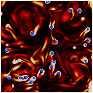
We may also confirm the  $St$ dependence of the relative velocity in visualizations. Figure 4 shows snapshots of flow and particle motions on a cross-section ( $z=0$) for Run 256v. Black arrows show the flow, which is composed of four vortex columns sustained by $\boldsymbol {f}^{(v)}$, (2.3), whereas blue balls are the particles ( $D=0.17\overline{L}$) with two different $St$ values: $St=0.51$ in figure 4(a), and $St=130$ in figure 4(b). Comparing the particle velocity (blue arrows) to the fluid velocity, we can see that the relative velocity is much more significant for the larger $St$. It is also remarkable that large enstrophy is produced in the wakes of the particles with larger $St$. As will be explained below, this large relative velocity and the resulting vortex shedding in large $St$ cases are the cause of the turbulence attenuation.

Figure 4. Visualization of flow and particle motions on the  $z=0$ plane for Run 256v. Blue balls indicate particles, $D=0.17\overline{L}$ ( $=7.8\overline{\eta }$); blue arrows indicate particle velocity; black arrows indicate fluid velocity; background colour indicates enstrophy magnitude (redder colour implies larger magnitudes). The Stokes number is (a) $St=0.51$ and (b) $St=130$. A supplementary movie is also available online at https://doi.org/10.1017/jfm.2022.787.
Since we have computed the relative velocity, we can estimate the energy dissipation rate per unit mass due to the shedding vortices around particles by
 \begin{equation} \epsilon_p=C_p\varLambda\,\frac{\overline{\langle|{\rm \Delta}\boldsymbol{u}|^{3}\rangle_p}}{D}. \end{equation}
Here,  $C_p$ is a constant, and $\varLambda$ is the volume fraction of the particles. The estimation (3.1) of $\epsilon _p$ is derived under the assumption that the energy dissipation rate in the wake behind a single particle is balanced with the energy input rate $P_p$ due to the force from the particle to fluid. Since $P_p$ depends only on $D$ and $|{\rm \Delta} \boldsymbol {u}|$ when the particle Reynolds number $Re_p$ (see (3.3) below) is large, the dimensional analysis leads to $P_p\sim |{\rm \Delta} \boldsymbol {u}|^{3}/D$. Then the mean energy dissipation rate due to all particles may be estimated by (3.1) with the factor $\varLambda$ because the volume fraction of particle wakes is proportional to $\varLambda$. The estimation of $\epsilon _p$ by (3.1) is an approximation because, in a more precise sense, $C_p$ weakly depends on $Re_p$. This approximation is, however, sufficient in the following arguments. The additional energy dissipation rate $\epsilon _p$ is the key quantity for understanding the turbulence attenuation. More concretely, when the relative velocity is non-negligible, shedding vortices enhance turbulent fluctuating velocity at scales smaller than the particle size $D$. This enhancement was demonstrated in previous studies (ten Cate et al. Reference ten Cate, Derksen, Portela and Akker2004; Yeo et al. Reference Yeo, Dong, Climent and Maxey2010; Wang et al. Reference Wang, Ayala, Gao, Andersen and Mathews2014) by investigating the energy spectrum. In particular, they showed that the energy spectrum $E(k)$ was enhanced (attenuated) for wavenumbers $k$ larger (smaller) than the pivot wavenumber $k_p\approx 0.6k_d$– $0.9k_d$, with $k_d=2{\rm \pi} /D$. In the present DNS, we may estimate $k_p$ in the case with the smallest particles because the other cases show only moderate attenuations. By estimating the energy spectrum without special treatments of the existence of particles, we observe that the smallest particles ( $D\approx 8\overline{\eta }$ in both Runs 256v and 256i) attenuate $E(k)$ for $k\lesssim 0.5k_d$, whereas they strongly enhance it for $k\gtrsim k_d$ (figures are omitted). These observations are consistent with the proposed scenario of turbulence attenuation; that is, particles acquire their energy from the largest energetic eddies and then bypass the energy cascading process to dissipate directly the energy at the rate $\epsilon _p$ in their wakes.
In fact, it is evident in figures 3(b) and 3(d) that the attenuation rate defined by
 \begin{equation} Ar=\frac{\overline{K'_0}-\overline{K'}}{\overline{K'_0}} \end{equation}
is approximately proportional to  $\epsilon _p$. This is the most important observation of the present DNS. We also show in figures 3(b,d) results (red symbols) with a smaller volume fraction ( $\varLambda =4.1\times 10^{-3}$) for the smallest particle cases. We can see that the relation between $Ar$ and $\epsilon _p$ is independent of $\varLambda$, which further verifies the estimation (3.1) of $\epsilon _p$. Note that the proportional coefficient $Ar/(\epsilon _p/\epsilon _0)$ is about twice as large for the turbulence driven by $\boldsymbol {f}^{(v)}$ as for $\boldsymbol {f}^{(i)}$. In the next section (see (4.10)), we will show the origin of this difference.
By using the estimated relative velocity magnitude, we can also estimate the particle Reynolds number
 \begin{equation} Re_p=\frac{D\,\overline{\langle|{\rm \Delta}\boldsymbol{u}|\rangle_p}}{\nu} \end{equation}
to see if  $Re_p$ is large enough for vortex shedding. The estimated values are listed in table 2. For example, for $St=32$, $Re_p=42$ for $D=0.17\overline{L}$, $Re_p=80$ for $D=0.33\overline{L}$, and $Re_p=124$ for $D=0.66\overline{L}$. This means that vortices are shedding from the particles in these cases. It is, however, important to emphasize that although $Re_p\gtrsim 1$ is a necessary condition for the turbulence attenuation, large $Re_p$ does not always imply a large attenuation rate, which depends on $D$.
$D$.
4. Discussions
On the basis of the DNS results shown in the previous section, we discuss the physical mechanism of turbulence attenuation in the present system. Figures 1 and 2 imply that turbulence can be attenuated more significantly by smaller particles, and no attenuation occurs when  $D/\overline{L}\approx 1$. Therefore, here we restrict ourselves to the cases of the attenuation by small particles; more precisely,
 \begin{equation} D\lesssim\overline{L}. \end{equation}
It is also an important observation that vortex shedding from particles is enhanced when turbulence is significantly attenuated (see figure 4 and the supplementary movie). This implies that when vortices are shed from particles smaller than  $\overline{L}$, the intrinsic turbulent energy cascade is bypassed and the energy dissipation is enhanced by the shedding vortices, which leads to the attenuation. In the following subsections, we consider the condition and degree of the turbulence attenuation due to this mechanism.
4.1. Condition for turbulence attenuation
Let us derive the condition for turbulence attenuation. For simplicity, in this subsection, we neglect the temporal fluctuations of  $L(t)$, $\lambda (t)$, $K'(t)$ and $u'(t)$, and omit the overbars of $\overline{L}$, $\overline{\lambda }$, $\overline {K'}$ and $\overline {u'}$. The DNS results shown in the previous section (see figures 3b,d) indicate that the attenuation rate is determined by the energy dissipation rate (3.1) due to shedding vortices. Therefore, turbulence attenuation requires the conditions for shedding vortices to acquire their energy from the turbulence: (i) there exists non-negligible (i.e. $O(u')$) relative velocity between particles and their surrounding fluid; and (ii) the particle Reynolds number (3.3) is large enough for shedding vortices.
First, we examine (i), which is the condition for particles not to follow the surrounding flow. In other words, the particle velocity relaxation time  $\tau _p$ is larger than the turnover time of the largest eddies, i.e. $St\gtrsim 1$. Estimating $\tau _p$ by (2.9), we can express this condition ( $St\gtrsim 1$) as
 \begin{equation} D\gtrsim\sqrt{\frac{18}{\gamma\,Re}}\,L\sim\frac{\lambda}{\sqrt{\gamma}}. \end{equation}
Here, we have defined the Reynolds number by  $Re=u'L/\nu$, and used $T=L/u'$ and the expression
 \begin{equation} \epsilon=\frac{15\nu u'^{2}}{\lambda^{2}}\sim \frac{u'^{3}}{L} \end{equation}
of the energy dissipation rate in isotropic turbulence (Taylor Reference Taylor1935).
Equation (4.2) implies that the sufficient velocity difference between particles and fluid requires that particle diameter  $D$ must be larger than a length proportional to the Taylor length $\lambda$. Note, however, that when the mass density ratio $\gamma$ is much larger than $1$, particles smaller than $\lambda$ can attenuate turbulence because of the coefficient $1/\sqrt {\gamma }$ on the right-hand side of (4.2). Indeed, this is the case for some parameters of the present DNS; for example, for Run 256v (see table 1), although $D=0.17{L}$ is comparable with $\lambda$, $St$ can be much larger than $1$ when $\gamma \gg 1$, and in such cases turbulence is significantly attenuated (figure 1).
Next, we examine condition (ii). When (4.2) holds, the relative velocity magnitude is  $O(u')$ (figures 3a,c), and therefore the particle Reynolds number (3.3) is $Re_p\approx u'D/\nu$. The condition for $Re_p$ to be larger than $O(1)$ is therefore expressed as
 \begin{equation} D\gtrsim L/Re. \end{equation}
For  $Re\gg 1$, if (4.2) holds, then (4.4) also holds. Hence (4.2) gives the lower bound of $D$ for the turbulence attenuation by small particles.
4.2. Estimation of attenuation rate
Further developing the above arguments, we may also estimate the attenuation rate of  $K'$. Here, we assume that if $D\ll L$, then particles have only limited impact on the mean flow; this is indeed the case in the present system with mean flow driven by $\boldsymbol {f}^{(v)}$. Under this assumption, the energy input rate $\langle \boldsymbol {U}\boldsymbol {\cdot }\boldsymbol {f}^{(v)}\rangle$ is the same as in the single-phase turbulence. Hence, because of the statistical stationarity, the mean energy dissipation rate of the particulate turbulence is approximately equal to the value
 \begin{equation} \epsilon_0=C_\epsilon\,\frac{(K_0+K'_0)^{3/2}}{L} \end{equation}
for the single-phase flow. Here,  $C_\epsilon$ ( $=O(1$)) is a flow-dependent constant (Goto & Vassilicos Reference Goto and Vassilicos2009), and $K_0$ and $K'_0$ denote the kinetic energies of the mean and fluctuating single-phase flows, respectively. Incidentally, in the turbulence driven by $\boldsymbol {f}^{(i)}$, although the mean flow is absent, the energy input rate is the same, by construction (2.4) of the forcing, in the single-phase and particulate flows.
In particulate turbulence with a small volume fraction of particles, the input energy is either transferred to the Kolmogorov scale by the energy cascading process from the forcing-scale eddies, or dissipated in the wake behind particles. Hence the energy dissipation rate is the sum of  $\epsilon _c$ through the energy cascade and $\epsilon _p$ in the wake of the particles (i.e. the energy dissipation rate bypassing the energy cascade):
 \begin{equation} \epsilon_0=\epsilon_c+\epsilon_p. \end{equation}
Here,  $\epsilon _c$ is expressed by
 \begin{equation} \epsilon_c=C_\epsilon\,\frac{(K_0+K')^{3/2}}{L} \end{equation}
in terms of the modulated turbulent kinetic energy  $K'$. Then substituting (4.5) and (4.7) into (4.6) divided by $\epsilon _0$, we obtain the formula
 \begin{equation} 1-\left(1-\frac{Ar}{1+\alpha}\right)^{3/2}=\frac{\epsilon_p}{\epsilon_0} \end{equation}
for the attenuation rate  $Ar$ defined by (3.2). In (4.8), $\alpha$ denotes the ratio
 \begin{equation} \alpha=\frac{K_0}{K'_0} \end{equation}
between the mean and fluctuation energies of single-phase flow:  $\alpha =0$ for the turbulence driven by $\boldsymbol {f}^{(i)}$, whereas $\alpha$ is estimated numerically as $1.86/1.89\approx 0.98$ for $\boldsymbol {f}^{(v)}$. Note that although $C_\epsilon$ in (4.5) and (4.7) depends on flow, (4.8) is independent of $C_\epsilon$. This means that (4.8) is flow-independent. In fact, by using (4.8), the two data sets of $Ar$ in figures 3(b) and 3(d) for the two kinds of forcing collapse (figure 5). The formula (4.8) further reduces to
 \begin{equation} Ar\sim\frac{(1+\alpha)\epsilon_p}{\epsilon_0} \end{equation}
when  $Ar$ is not too large. This explains the reason why the proportional constant $Ar/(\epsilon _p/\epsilon _0)$ in figure 3(b) is approximately twice as large as that in figure 3(d). Recall that $\alpha +1\approx 1.98$ for $\boldsymbol {f}^{(v)}$, and $\alpha +1=1$ for $\boldsymbol {f}^{(i)}$.

Figure 5. Verification of (4.8), according to which we replot the data in figures 3(b) and 3(d) with blue and black symbols, respectively. Darker and lighter symbols denote the cases with  $\varLambda =8.2\times 10^{-3}$ and $4.1\times 10^{-3}$, respectively. The dashed line indicates $1.3\epsilon _p/\epsilon _0$.
We emphasize that (4.8) can predict the attenuation rate  $Ar$ if we know $\epsilon _p$. By using (3.1), we may estimate $\epsilon _p$ for $St\gg 1$ because $|{\rm \Delta} \boldsymbol {u}|=cu'$ for $St\gg 1$ with a flow-dependent constant $c$ (figures 3a,c). Then we may rewrite (4.8) as
 \begin{equation} 1-\left(1-\frac{Ar}{1+\alpha}\right)^{3/2}=\frac{C_p'\varLambda L}{D}\quad (St\gg 1). \end{equation}
Here,  $C_p'\sim c^{3}C_p/C_\epsilon$ is also a flow-dependent constant. The above equation may reduce to
 \begin{equation} Ar\sim\frac{(1+\alpha)\varLambda L}{D}\quad (St\gg 1) \end{equation}
when  $Ar$ is not too large. This simple expression (4.12) means that the attenuation due to the considered mechanism occurs when (4.1) holds with a sufficient volume fraction $\varLambda$. In other words, the upper bound of the attenuation by small particles is given by (4.1). It also explains that the attenuation rate $Ar$ is larger for smaller $D$. Hence, combining this with (4.2), we conclude that for fixed $\varLambda$ and $\gamma$, particles with size proportional to $\lambda /\sqrt {\gamma }$ most effectively attenuate turbulence intensity. Since the numerical verification of this conclusion requires DNS with further smaller particles, we leave it for future studies. It is also worth mentioning that $\epsilon _p$ (see (3.1) and figures 3b,d), and therefore $Ar$ approximated by (4.12), are proportional to the volume fraction $\varLambda$. This explains the reason why larger mass fraction ( $\gamma \varLambda$) generally tends to lead larger turbulence attenuation because $St$ is larger for larger $\gamma$.
5. Conclusions
We have derived the conditions (4.1) and (4.2), i.e.  $\overline{L}\gtrsim D \gtrsim \overline{\lambda }/\sqrt {\gamma }$, for the dilute additives of solid spherical particles, without gravity, to attenuate turbulence in a periodic cube. First, we have verified numerically the conventional picture that the attenuation is due to the additional energy dissipation rate $\epsilon _p$ in (3.1), caused by shedding vortices around particles; more concretely, we have shown in figures 3(b) and 3(d) that the attenuation rate $Ar$ is approximately proportional to $\epsilon _p$. This result leads immediately to the attenuation condition because the attenuation occurs when $\epsilon _p$ in (3.1) takes a finite value, which requires a finite relative velocity $|{\rm \Delta} \boldsymbol {u}|$ between particles and their surrounding fluid, i.e. $St\gtrsim 1$. In fact, as shown in figures 3(a) and 3(c), $|{\rm \Delta} \boldsymbol {u}|$ takes finite values when $St\gtrsim 1$, and it tends to a value of $O(u')$ for $St\gg 1$. The condition $St\gtrsim 1$ leads to (4.2) for the particle diameter $D$; and if (4.2) holds, then $Re_p\gg 1$ also holds, and therefore vortices are shedding from the particles. Hence (4.2) gives the lower bound of $D$ for the turbulence attenuation. In other words, since particles smaller than $\overline{\lambda }/\sqrt {\gamma }$ behave like tracers for the largest energetic eddies, they cannot modulate them.
The picture of the turbulence attenuation due to the shedding vortices also leads to the estimation of the attenuation rate. The simple argument developed in § 4.2 leads to (4.8), which well explains the DNS results (figure 5). We emphasize that (4.8) is a formula independent of forcing schemes. For  $St\gg 1$, (4.8) reduces to $Ar\sim {\varLambda \overline{L}}/{D}$ (see (4.12)), which implies that for a given volume fraction, smaller particles that satisfy (4.2) attenuate turbulence more effectively. This is consistent with the DNS results (figures 1 and 2). Hence in turbulence at sufficiently high Reynolds numbers (and therefore $\overline{L}\gg \overline{\lambda }\gg \overline{\eta }$), particles with size proportional to $\overline{\lambda }/\sqrt {\gamma }$ attenuate turbulence most significantly under the condition that the Reynolds number $Re$, the mass ratio $\gamma$ and the volume fraction $\varLambda$ are fixed. Furthermore, since $Ar$ is proportional to $\varLambda \overline{L}/D$ for $St\gg 1$, turbulence is hardly attenuated when $D$ is as large as $\overline{L}$ (see also figures 1 and 2). Therefore, (4.1) gives the upper bound of $D$ for the attenuation by the considered mechanism.
Recall that we have considered turbulence attenuation only by small particles. Although it is difficult to conduct DNS with particles larger than  $\overline{L}$ in turbulence at similar Reynolds numbers, we may expect only small relative velocity for $D\gtrsim \overline{L}$ in the present system, where neither gravity nor mean flow larger than $\overline{L}$ exists. Then vortices are not shed from such large particles. Incidentally, when the mean-flow or gravitational effects are important, the relative velocity between particles and fluid creates vortices, which can lead to turbulence modulation.
Before closing this paper, it is worth mentioning the possibility that particles can modulate turbulence even if they do not satisfy (4.2) because they can interrupt energy cascade in the inertial range. More concretely, if particles’ velocity relaxation time  $\tau _p$ is comparable with the turnover time $\tau (\ell )$ of eddies with size $\ell$ in the inertial range, then they follow the motion of eddies larger than $\ell$, but they have relative velocity with those smaller than $\ell$. Since larger eddies have more energy, the relative velocity between particles and fluid is determined by the eddies with size $\ell$. Therefore, the particles acquire their energy from such eddies with size $\ell$ and some part of cascading energy at scales smaller than $\ell$ may be bypassed by the shedding vortices behind particles and dissipated in the wake of particles. Such a phenomenon is to be observed numerically in turbulence at higher Reynolds numbers in the near future.
Supplementary movie
A supplementary movie is available at https://doi.org/10.1017/jfm.2022.787.
Acknowledgements
The DNS were conducted with the support of the NIFS Collaboration Research Program (20KNSS145) and the supercomputer Fugaku provided by RIKEN through the HPCI System Research projects (hp210207). S.G. thanks the late professor Michio Nishioka for relevant discussions in the laboratory.
Funding
This study was partly supported by JSPS Grant-in-Aids for Scientific Research (20H02068).
Declaration of interests
The authors report no conflict of interest.


 Open access