


1. Introduction
Turbulence is known to be stochastic, but its statistics are expected to reflect the symmetries that constrain it. An example is the flat-plate boundary layer, where the flow is statistically symmetric in the spanwise direction owing to the statistical homogeneity. Symmetry properties of turbulence like the one above have received considerable empirical support and are common in fluid flow modelling (Pope Reference Pope2000). In recent developments of machine learning models, constraints such as symmetry or invariance properties are invoked to improve the training efficiency (Ling, Kurzawski & Templeton Reference Ling, Kurzawski and Templeton2016; Duraisamy, Iaccarino & Xiao Reference Duraisamy, Iaccarino and Xiao2019; Brunton, Noack & Koumoutsakos Reference Brunton, Noack and Koumoutsakos2020). Deviations from symmetry considerations are often attributed to a lack of statistical convergence or numerics. For instance, Grandemange, Gohlke & Cadot (Reference Grandemange, Gohlke and Cadot2013, Reference Grandemange, Gohlke and Cadot2014) found asymmetry in a wake flow, but the asymmetry vanishes when the averaging time is sufficiently long. The goal of this work is to test such symmetry considerations in the context of flow over aligned cube arrays.
1.1. Roughness-induced large-scale secondary flows
The dominant dynamics within a flat-plate boundary layer are characterized by self-sustaining cycles in the inner layer (Jimenez & Moin Reference Jiménez and Moin1991), as well as the presence of large-scale motions (Adrian Reference Adrian2007; Hutchins & Marusic Reference Hutchins and Marusic2007) and very-large-scale motions in the outer layer (Kim & Adrian Reference Kim and Adrian1999; Balakumar & Adrian Reference Balakumar and Adrian2007; Dennis & Nickels Reference Dennis and Nickels2011a,Reference Dennis and Nickelsb). However, the introduction of surface roughness disrupts the self-sustaining cycle, transforming the inner layer into the roughness sublayer. Within this sublayer, the flow is a combination of roughness wakes and a shear layer riding atop the roughness elements (Yang et al. Reference Yang, Sadique, Mittal and Meneveau2016; Aghaei-Jouybari et al. Reference Aghaei-Jouybari, Seo, Yuan, Mittal and Meneveau2022; Zhang et al. Reference Zhang, Zhu, Yang and Wan2022). The roughness sublayer extends approximately 3–5 times the roughness height (Raupach, Antonia & Rajagopalan Reference Raupach, Antonia and Rajagopalan1991; Flack, Schultz & Connelly Reference Flack, Schultz and Connelly2007). Beyond the roughness sublayer, the flow characteristics resemble those of a flat-plate boundary layer (Jiménez Reference Jiménez2004; Castro Reference Castro2007; Schultz & Flack Reference Schultz and Flack2007; Leonardi & Castro Reference Leonardi and Castro2010; Flack & Schultz Reference Flack and Schultz2014; Chung, Monty & Hutchins Reference Chung, Monty and Hutchins2018; Chung et al. Reference Chung, Hutchins, Schultz and Flack2021).
In the past decade, significant attention has been devoted to studying roughness-induced secondary motions that extend beyond the roughness sublayer. Pioneering studies by Mejia-Alvarez & Christensen (Reference Mejia-Alvarez and Christensen2013) and Barros & Christensen (Reference Barros and Christensen2014) were among the first to report these secondary motions. In their investigations, these large-scale secondary motions manifest as spanwise alternating high- and low-momentum pathways in the mean flow. Similar secondary motions have been observed above herringbone-like roughness (Nugroho, Hutchins & Monty Reference Nugroho, Hutchins and Monty2013), spanwise alternating high- and low-roughness stripes (Willingham et al. Reference Willingham, Anderson, Chritensen and Barros2014), and spanwise heterogeneous super-hydrophobic surfaces (Jelly, Jung & Zaki Reference Jelly, Jung and Zaki2014; Lee, Jelly & Zaki Reference Lee, Jelly and Zaki2015). Moreover, similar secondary motions arise in other contexts. In fact, secondary motions arise as long as the Reynolds stresses are spanwise heterogeneous (Anderson et al. Reference Anderson, Barros, Christensen and Awasthi2015). The strength of these large-scale secondary motions is by and large determined by the length scale of the spanwise heterogeneity (Vanderwel & Ganapathisubramani Reference Vanderwel and Ganapathisubramani2015; Chan et al. Reference Chan, MacDonald, Chung, Hutchins and Ooi2018; Yang & Anderson Reference Yang and Anderson2018; Yang et al. Reference Yang, Xu, Huang and Ge2019). The secondary motions are the strongest when the spanwise length scale is comparable to the boundary-layer height. Other factors also affect the strength of the secondary motions. The impacts of thermal stratification, roughness geometry and roughness arrangements have been investigated by Forooghi, Yang & Abkar (Reference Forooghi, Yang and Abkar2020), Medjnoun, Vanderwel & Ganapathisubramani (Reference Medjnoun, Vanderwel and Ganapathisubramani2020) and Viggiano et al. (Reference Viggiano, Bossuyt, Ali, Meyers and Cal2022), respectively. Nonetheless, the aforementioned studies did not report statistically significant asymmetries in the mean flow, which is the focus of our current investigation.
1.2. This work
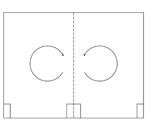
We consider flow above aligned cubes as shown in figure 1(a). Aligned cubes induce secondary flows of the second kind, which manifest as counter-rotating vortices, as depicted in figure 1(b). The direction of these secondary flows, whether they bring low- or high-momentum fluid to the cubes, depends on the surface coverage density (Vanderwel & Ganapathisubramani Reference Vanderwel and Ganapathisubramani2015; Xu et al. Reference Xu, Altland, Yang and Kunz2021). In figure 1, the secondary motions bring high-momentum fluid to the cubes. These secondary flows are part of the mean flow, and they are expected to exhibit the symmetry that constrains flow. Specifically, the secondary flows should possess spanwise symmetry, with the symmetry plane indicated by the vertical dashed line across the cube centre in figure 1(b). Empirical evidence strongly supports this anticipated symmetry (Coceal et al. Reference Coceal, Thomas, Castro and Belcher2006; Cheng et al. Reference Cheng, Hayden, Robins and Castro2007; Cheng & Porté-Agel Reference Cheng and Porté-Agel2015; Yang Reference Yang2016; Yang et al. Reference Yang, Sadique, Mittal and Meneveau2016; Basley, Perret & Mathis Reference Basley, Perret and Mathis2019; Xu et al. Reference Xu, Altland, Yang and Kunz2021). In this paper, we aim to re-evaluate this expected symmetry using direct numerical simulations (DNS).

Figure 1. (a) A sketch of the cubical roughness, where  $x$,
$x$,  $y$,
$y$,  $z$ are the streamwise, spanwise and vertical directions, respectively, $h$ is the roughness height, and $s$ is the spacing between adjacent roughness elements. The roughness is arranged in an aligned configuration. (b) A sketch of the roughness-induced large-scale secondary vortices in the spanwise-vertical ( $y$–
$y$– $z$) plane. The vertical dashed line across the cube centre shows the symmetry plane.
The remainder of the paper is organized as follows. In § 2, we provide a detailed description of the DNS set-up. We employ an averaging time that exceeds the typical duration used in prior DNS studies of rough-wall boundary-layer flows. The results are presented in § 3. In § 4, we demonstrate that the observed asymmetry persists across variations in numerical techniques, domain sizes, the arrangement of cubes in the spanwise direction, and Reynolds numbers. Finally, concluding remarks are provided in § 5.
2. Direct numerical simulations
Creating a perfectly symmetric laboratory facility can be a challenging, if not impossible, task. However, such limitations are non-existent in numerical simulations. In our study, we conduct DNS of a half-channel flow with cubical roughness on the bottom wall.
For our DNS, we utilize the pseudo-spectral code LESGO, which solves the incompressible Navier–Stokes equations. The code employs a pseudo-spectral method in the streamwise and spanwise directions, while using a second-order finite difference method in the wall-normal direction. The domain is periodic in the streamwise and spanwise directions, with a stress-free top boundary. To resolve the roughness, we employ an immersed boundary method (Chester, Meneveau & Parlange Reference Chester, Meneveau and Parlange2007). The code has been extensively validated and used for simulating boundary-layer flows, including those over complex terrains (Anderson et al. Reference Anderson, Barros, Christensen and Awasthi2015; Yang & Meneveau Reference Yang and Meneveau2016, Reference Yang and Meneveau2017), vegetative canopies (Chester et al. Reference Chester, Meneveau and Parlange2007; Bai, Meneveau & Katz Reference Bai, Meneveau and Katz2012) and urban canopies (Cheng & Porté-Agel Reference Cheng and Porté-Agel2015; Giometto et al. Reference Giometto, Christen, Meneveau, Fang, Krafczyk and Parlange2016; Yang et al. Reference Yang, Xu, Huang and Ge2019; Zhang et al. Reference Zhang, Zhu, Yang and Wan2022). Further details of the code are omitted here for the sake of brevity.
Table 1 provides an overview of our DNS set-up. We consider aligned cube arrays as the surface roughness, with a surface coverage density or solidity ranging from  $0.25\,\%$ to $6.25\,\%$. The domain height $L_z=6h$ is fixed, while the streamwise and spanwise dimensions of the domains satisfy $L_x\ge 2{\rm \pi} {L_z}$ and $L_y\ge {\rm \pi}{L_z}$ (Lozano-Durán & Jiménez Reference Lozano-Durán and Jiménez2014). The grid is uniform in the horizontal directions, with fixed grid spacing $\Delta x^+=\Delta y^+=3.75$. In the vertical direction, the grid is stretched to achieve resolution $\Delta z^+_{min}\approx 0.5$ near the wall and $\Delta z^+_{max}\approx 3$ at the top of the domain. This grid resolution is comparable to, and often finer than, that used in previous works (Coceal et al. Reference Coceal, Thomas, Castro and Belcher2006; Leonardi & Castro Reference Leonardi and Castro2010; MacDonald et al. Reference MacDonald, Ooi, García-Mayoral, Hutchins and Chung2018). In all DNS, the surfaces of the cubes coincide with the surfaces of the computational cells to give an accurate representation of the cube geometry.
Table 1. DNS details. The domain is a half-channel;  $Re_{\tau }=L_z u_\tau /\nu$ is the friction Reynolds number, where $u_\tau$ is the friction velocity; $s$ and $h$ are the spacing and height of cubical roughness elements, respectively; $\lambda _p$ is the surface roughness coverage density; $L_x$, $L_y$ and $L_z$ are the sizes of the domain in the streamwise, spanwise and wall-normal directions, respectively; $n_x \times n_y$ are the sizes of the cube array; and $\Delta x^+$, $\Delta y^+$ and $\Delta z^+$ are the grid spacings in the three directions normalized by viscous scales. The grid is uniform in horizontal directions and stretched in the vertical direction; $T$ is statistical time; and $U_0$ is the mean streamwise velocity at the top of the domain. S10X1, S10X2 differ in their roughness arrangements.

Our baseline cases are denoted as S $[s/h]$, where $s$ represents the spacing between neighbouring cubes, and $h$ denotes the cube height. We vary $s$ from $4h$ to $20h$, resulting in cases S04, S06, S08, S10, S13, S15 and S20. Additionally, we explore variations in the initial condition and domain size. This leads to S13R, which involves flipping the spanwise coordinate of S13 to verify that any observed mean flow asymmetry is not an artefact of the numerics, and S13X1 and S13X2, where we double and quadruple the streamwise size of the S13 domain, respectively, to confirm the robustness of the observed asymmetry to changes in domain dimensions. To study the effects of the spanwise size of the domain, we add cases S10X1, S10X2 and S13X1, where we double the spanwise size of the S10 and S13 domains. Finally, we investigate the effect of cube placement in the spanwise direction, resulting in cases S10X1 and S10X2, where the roughness in S10X2 is shifted spanwise relative to S10X1. The purpose of these cases is to demonstrate that the location of the cubes does not influence the observed asymmetry.
The S[ $s$] cases are conducted at a friction Reynolds number $Re_{\tau }=360$, where $u_{\tau }=\sqrt {(1/\rho ) L_z \,{\rm d}P/{{\rm d} x}}$ represents the friction velocity, $L_z$ is the height of the half-channel, ${\rm d}P/{{\rm d}x}$ is the pressure gradient driving the flow, and $\rho$ is the fluid density. To examine whether the observed asymmetry is unique to a specific Reynolds number, we perform additional five DNS at $Re_{\tau }=180$, denoted as L06, L08, L10, L15 and L20. These lower Reynolds number simulations are chosen as the flow is already in the fully rough regime at $Re_{\tau }=360$, and increasing the Reynolds number is unlikely to significantly alter the flow phenomena. We use an averaging time ranging between 80 and 120 large-eddy turnover times, where $L_z/u_\tau$ corresponds to one large-eddy turnover time. Table 2 provides a summary of the averaging times used in some of the prior DNS studies of rough-wall boundary layers. The typical averaging time is 10–50 large-eddy turnover times, except that $100L_z/u_\tau$ is used by Coceal et al. (Reference Coceal, Thomas, Castro and Belcher2006), which is comparable to our averaging time. Our chosen averaging time is longer than the typical averaging time and is twice as long as what Yuan & Piomelli (Reference Yuan and Piomelli2014) considered sufficient for obtaining converged mean flow statistics.
Table 2. Averaging time used in prior DNS studies of rough-wall boundary-layer flows. Here,  $\delta /u_\tau$ is large-eddy turnover time, where $\delta$ is half-channel height/boundary layer thickness/pipe radius. This is not meant to be a comprehensive list.

3. Results
We present the results of the baseline cases in this section. Figure 2 shows the contours of the streamwise and temporally averaged velocities  ${\langle {\bar u} \rangle _{x}}$ in the spanwise–vertical ( $y$–
$y$– $z$) plane. The in-plane motions are shown via $({\langle {\bar v} \rangle _{x}},{\langle {\bar w} \rangle _{x}})$ vectors. Here, $u$,
$u$,  $v$,
$v$,  $w$ are the velocities in the streamwise ( $x$), spanwise ( $y$) and vertical ( $z$) directions, respectively, the overbar denotes time averaging, $\langle \cdot \rangle$ denotes spatial average, and the subscript is the direction of averaging. The symmetry plane is located at the cube centre ( $y=0$). Large-scale secondary motions that span the entire boundary layer are found when $s/h>6$. In S04, S06 and S20, the secondary motions are approximately symmetric with respect to $y=0$, which aligns with previous findings. Previous authors have also reported spanwise symmetric mean flow above aligned cubes with surface coverage density $\gtrsim 3\,\%$ (Yang et al. Reference Yang, Sadique, Mittal and Meneveau2016; Xu et al. Reference Xu, Altland, Yang and Kunz2021), which corresponds to S04 and S06 in our study. Additionally, the flow above isolated cubes, a good approximation for case S20, is known to exhibit spanwise symmetry (Wang & Lam Reference Wang and Lam2019).

Figure 2. Contours of the streamwise and temporally averaged streamwise velocity  $\langle {\bar u} \rangle _{x}$ in the spanwise/wall-normal plane. The velocity is normalized by its average at the top boundary, which we denote as $U_0$. The vectors indicate the in-plane motions, i.e. $({\langle {\bar v} \rangle _{x}},{\langle {\bar w} \rangle _{x}})$. The origin of the spanwise coordinate is placed at the centre of the roughness element. The roughness is symmetric with respect to $y=0$. The spanwise extent of the plot equals the distance between two neighbouring roughness elements, which is the minimum repeating unit of the flow. Cases are (a) S04, (b) S06, (c) S08, (d) S10, (e) S13, ( f) S15, and (g) S20.
However, what is unexpected is the spanwise asymmetry in the mean flows in cases S08, S10, S13 and S15. In these cases, we observe a significant vortex on one side of the roughness, while no such large vortex is present on the other side. These secondary vortices enhance the vertical transport of streamwise momentum, resulting in the spanwise undulation of  ${\langle {\bar u} \rangle _{x}}$ as revealed by the contour plots.
To obtain a more quantitative measure of the mean flow asymmetry, we examine the velocities on the symmetry plane at  $y=0$. Figure 3 displays the streamwise and temporally averaged velocities at the cube centre ( $cc$), denoted as $\langle {\bar u} \rangle _{x,cc}$, $\langle {\bar v} \rangle _{x,cc}$ and $\langle {\bar w} \rangle _{x,cc}$. In a symmetric flow with respect to $y=0$, the spanwise velocity $\langle {\bar v} \rangle _{x,cc}$ would be zero at $y=0$. As seen in S04 and S06, where the flow exhibits spanwise symmetry, $\langle {\bar v} \rangle _{x,cc}$ is indeed close to zero at $y=0$. However, in cases S10, S13 and S15, there is a noticeable deviation of $\langle {\bar v} \rangle _{x,cc}$ from zero, indicating the presence of mean flow asymmetry. While not as prominent as in cases S10 or S15, a non-zero value of $\langle {\bar v} \rangle _{x,cc}$ is also observed in S20, indicating a weak mean flow asymmetry in this case. The behaviours of $\langle {\bar u} \rangle _{x,cc}$ and $\langle {\bar w} \rangle _{x,cc}$ align with findings reported in the literature. Specifically, $\langle {\bar u} \rangle _{x,cc}$ increases with increasing inter-cube distance due to the decreasing drag force in the k-type roughness regime. This trend is consistent with previous studies. In terms of $\langle {\bar w} \rangle _{x,cc}$, a downwelling motion leads to a negative value in cases S08, S10, S13, S15 and S20, similar to the observations made by Willingham et al. (Reference Willingham, Anderson, Chritensen and Barros2014), Anderson et al. (Reference Anderson, Barros, Christensen and Awasthi2015) and Chung et al. (Reference Chung, Monty and Hutchins2018). On the other hand, an upwelling motion results in a positive $\langle {\bar w} \rangle _{x,cc}$ in S04, which is in line with the findings of Xu et al. (Reference Xu, Altland, Yang and Kunz2021).

Figure 3. Streamwise and temporally averaged velocities at the cube centreline (i.e.  $y=0$ in figure 2): (a) $\langle {\bar u} \rangle _{x,cc}/u_\tau$, (b) $\langle {\bar v} \rangle _{x,cc}/u_\tau$, and (c) $\langle {\bar w} \rangle _{x,cc}/u_\tau$.
Figures 4(a–g) show the streamwise, wall-normal and time-averaged  $x$ velocity $\left \langle \bar {u}\right \rangle _{x,z}/U_b$ as a function of the spanwise coordinate, which is also a good measure of the mean flow asymmetry. Here, $U_b=\left \langle \bar {u}\right \rangle _{x,y,z}$ is the mean flow rate. We see that the flow is roughly spanwise symmetric in S04, S06 and S20, and spanwise asymmetric in S08, S10, S13 and S15. The dip at $y=0$ is due to the roughness that blocks the flow. The other dips in the S08, S10, S15 and S20 results are due to secondary motions, which bring low-speed fluid in the wake of the cube to its sides.

Figure 4. Streamwise and normal averaged mean velocity  $\left \langle \bar {u}\right \rangle _{x,z}$ as a function of the spanwise coordinate for (a) S04, (b) S06, (c) S08, (d) S10, (e) S13, ( f) S15, and (g) S20. We show results in one repeating unit for brevity. The origin of the spanwise coordinate is at the centre of the roughness element.
Finally, we define
 \begin{equation} \Delta U(y)\equiv\left|\left\langle\bar{u}\right\rangle_{x,z}(y)-\left\langle\bar{u}\right\rangle_{x,z}({-}y) \right|, \end{equation}
and  $\max _y[\Delta U]$ and $\left \langle [\Delta U]\right \rangle _y$, i.e. the maximum of $\Delta U$ and the average of $\Delta U$, are one-number measures of the mean flow asymmetry, with $\Delta U(y)=0$ if the flow is spanwise symmetric. Figure 5 shows $\left \langle \Delta U\right \rangle _y$ and $\max _y[\Delta U]$ as functions of the inter-cube distance $s$. Both measures are approximately 0 in S04 and S06. They increase as $s/h$ increases, and peak when $s/h=15$. The peak values are 0.07 and 0.12 for $\left \langle [\Delta U]\right \rangle _y/U_b$ and $\max _y[\Delta U]/U_b$, respectively, suggesting that the asymmetry can be as large as 10 % of the bulk velocity.

Figure 5. The maximum (square symbols) and the mean (triangle symbols) of  $\Delta U/U_b$ as a function of the inter-cube distance.
4. Discussion
4.1. Numerics, domain size and Reynolds number
In this subsection, we show that the mean flow asymmetry is robust to variations in the domain size, the direction of the spanwise axis, the spanwise location of the surface roughness, the initial condition, and the Reynolds number.
In our case, the averaging time exceeds 100 large-eddy turnover times. We examine the momentum budget and the premultiplied velocity probability density function (p.d.f.). Consider a generic flow quantity  $\phi$. Time averaging is sufficient if $\partial \bar {\phi }/\partial t = 0$, i.e. if the other terms in the $\phi$ transport equation balance. The transport equation of the streamwise velocity reads
 \begin{equation} \frac{{\rm d}\langle\bar{u}\rangle_{x,y}}{{\rm d} t}={-}\left\langle\frac{1}{\rho}\,\frac{\partial \bar{p}}{\partial x}\right\rangle_{x,y}-\frac{{\rm d}\langle\overline{u'w'}\rangle_{x,y}}{{\rm d} z}-\frac{{\rm d}\langle\overline{u''w''}\rangle_{x,y}}{{\rm d} z}+\nu\,\frac{{\rm d}^2 \langle\bar{u}\rangle_{x,y}}{{\rm d} z^2} \end{equation}
outside the roughness occupied layer, where  $u''=u-\langle \bar {u}\rangle _{x,y}$ and $w''=w-\langle \bar {w}\rangle _{x,y}$. The terms on the right-hand side are the mean pressure gradient term, the turbulent stress term, the dispersive stress term and the viscous stress term. If time averaging is sufficient, then the terms on the right-hand side should balance, leading to
 \begin{equation} {-}\langle\overline{u'w'}\rangle_{x,y}^+{-}\langle\overline{u''w''}\rangle_{x,y}^+{+}\frac{1}{Re_\tau}\,\frac{{\rm d} \langle\bar{u}\rangle_{x,y}^+}{{\rm d} z^+}=1-\frac{z}{L_z}, \end{equation}
which indicates that the sum of Reynolds stress, dispersive stress and viscous stress is a linear function of the wall-normal coordinate  $z$. This balance is confirmed by the results shown in figure 6. In addition to the momentum budget, we evaluate the averaging time through the premultiplied velocity p.d.f. (Meneveau & Marusic Reference Meneveau and Marusic2013; de Silva et al. Reference de Silva, Krug, Lohse and Marusic2017). Figure 7 shows the premultiplied p.d.f. of $u'$,
$u'$,  $v'$,
$v'$,  $w'$ in case S13 at two locations, i.e. $z/h=5$ and $z/h=3$, above the cube centre. We see that the mean flow, which is the area under the curve, is captured accurately. The results are similar at other locations and in other cases, and are not shown here for brevity. Nonetheless, further investigation may still be needed to confirm the statistical convergence.

Figure 6. Terms in (4.2), i.e. the momentum budget equation, for (a) S04, (b) S06, (c) S08, (d) S10, (e) S13, ( f) S15, and (g) S20. Here, Tot, Vis, Disp and Turb are short for total stress, viscous stress, dispersive stress and turbulent stress.

Figure 7. Premultiplied probability density functions of velocity fluctuations  $u'\,p(u')$, $v'\,p(v')$, $w'\,p(w')$ at (a–c) $z/h=3$ and (d–f) $z/h=5$ above the cube centre in case S13. The premultiplied probability density function has been normalized such that the maximum is 1.
Next, we explore the effects of inverting the spanwise axis to examine the sustainability of the observed asymmetry. According to the spanwise symmetry of the Navier–Stokes equations, if the asymmetry is inherent to the flow, then flipping the  $y$ axis and the spanwise velocity components should result in sustained asymmetry. We define the flipped quantities as
 \begin{gather} u_{flip}(x,y,z)=u(x,-y,z),\quad v_{flip}(x,y,z)={-}v(x,-y,z),\quad w_{flip}(x,y,z)=w(x,-y,z). \end{gather}
If numerics are responsible for the asymmetry, then  ${\boldsymbol u}_{flip}$ would not be able to sustain itself and would revert back to ${\boldsymbol u}$. Flipping the $y$ axis and the spanwise velocity in case S13 leads to case S13R. Figure 8 shows the contours of $\langle {\bar u}\rangle _{x}$ in S13R. The mean asymmetry sustains for more than another 100 large-eddy turnover times. Consequently, we conclude that numerics are not responsible for the observed asymmetries.

Figure 8. Same as figure 2, but for S13R.
Third, we investigate the effect of domain size. The size of our domain is comparable to those in the literature (Lozano-Durán & Jiménez Reference Lozano-Durán and Jiménez2014; Yang et al. Reference Yang, Xu, Huang and Ge2019; Xu et al. Reference Xu, Altland, Yang and Kunz2021) and should be sufficient. To further verify the adequacy of our domain size, we conduct two additional DNS: S13X1 with a domain twice as long and twice as wide as that of S13, and S13X2 with a domain four times as long as that of S13. Figures 9(a,b) show the contours of the mean flow, and the same asymmetry is observed. Hence we conclude that the finite domain size is not a concern.

Figure 9. Same as figure 2, but for (a) S13X1, (b) S13X2. Here, we show the full extent of the domain in the spanwise direction.
Fourth, we investigate the effect of the spanwise location of the cubes. Figure 10 shows the contours of the mean velocity in S10X1 and S10X2, where the cubes in S10X2 are displaced in the spanwise direction by 0.25 $s$ relative to S10X1. We see that the mean flow asymmetry persists, suggesting that spanwise location of the cubes should not affect the mean flow asymmetry. The result here also shows that the implementation of the periodic boundary condition in the spanwise direction does not affect the mean flow asymmetry.

Figure 10. Same as figure 2, but for (a) S10X1, (b) S10X2. Here, we show the full extent of the domain in the spanwise direction.
Finally, we investigate the effect of the Reynolds number. Figure 11 shows the results at  $Re_\tau =180$. We see that mean flow asymmetry exists at this low Reynolds number.

Figure 11. Same as figure 2, but for the  $Re_{\tau }=180$ cases: (a) L06, (b) L08, (c) L10, (d) L15, and (e) L20.
4.2. A heuristic explanation
Here, we attempt to explain the spanwise asymmetry in the mean flow. We know that the sizes of the secondary motions are constrained by both the height of the channel and the distance  $s$ between two neighbouring cubes (Vanderwel & Ganapathisubramani Reference Vanderwel and Ganapathisubramani2015). When $s$ is sufficiently large, the sizes of the secondary motions are limited by the channel half-height, and its size is $O(L_z)$ – this is what we see in S20. In that case, a repeating unit that spans a distance $s$ in the spanwise direction fits two secondary vortices, and the flow is spanwise symmetric. We call these secondary vortices developed vortices. When $s$ is sufficiently small, the sizes of the secondary motions are limited by $s$ – this is what we see in S06. A repeating tile that spans a distance $s$ in the spanwise direction also fits two of these secondary vortices, and again, the flow would be spanwise symmetric. We call these secondary vortices undeveloped vortices. When $s$ is such that it does not fit two developed vortices but is too large for two undeveloped vortices, a repeating tile would fit one developed vortex and one undeveloped vortex, thereby giving rise to the asymmetry that we see in the previous subsection.
4.3. Implication on the instantaneous flow field
The discussion so far has focused on the secondary flows, which are mean flow features. In this subsection, we discuss the implication of the mean flow asymmetry on the instantaneous flow structures, which are large-scale motions, very-large-scale motions, and super-structures in a boundary layer. These structures extend in the streamwise direction from a few boundary-layer heights to a few hundred boundary-layer heights (Kim & Adrian Reference Kim and Adrian1999; Guala, Hommema & Adrian Reference Guala, Hommema and Adrian2006; Balakumar & Adrian Reference Balakumar and Adrian2007; Hutchins & Marusic Reference Hutchins and Marusic2007; Monty et al. Reference Monty, Stewart, Williams and Chong2007; Kevin, Monty & Hutchins Reference Kevin, Monty and Hutchins2019). They are the most energetic motions in a boundary layer and are responsible for a lot of physical processes in a boundary layer (Smits, McKeon & Marusic Reference Smits, McKeon and Marusic2011; Marusic & Monty Reference Marusic and Monty2019). The asymmetry found in this work provides a potential strategy to control these structures: one can place the roughness such that these motions appear less frequently in one region and more frequently in another.
Figure 12 is a visualization of the instantaneous flow field at  $z/h=2$ in case S13 at eight time instances that are equally spaced over an extended period of time. We highlight the high-speed streaks following the methodology in Kevin et al. (Reference Kevin, Monty and Hutchins2019). We see that the high-speed streaks are more likely to appear on one side of the roughness elements than the other. Figure 13 shows the probability density function for observing a high-speed streak at a given $y$ location. We see that we can skew the probability density function significantly in S08, S10, S13 and S15, making the high-speed steaks appear on one side more frequently than on the other side.

Figure 12. Contours of the instantaneous velocity  $u/u_\tau$ at $z/h=2$ in S13, and between them, the time history of the horizontally averaged instantaneous wall shear stress ${\langle {{{ {\tau _w}} }} \rangle _{x,y}}/{\langle {{\overline {\tau _w} }} \rangle _{x,y}}$. The centrelines of the high-speed streaks are marked with the black lines in the contours. The squares show the locations of the cubes.

Figure 13. The occurrence probability of encountering a high-speed streak at a  $y$ location: (a) S04, (b) S06, (c) S08, (d) S10, (e) S13, ( f) S15, and (g) S20. The probability has been normalized.
5. Concluding remarks
We conduct DNS of flow over aligned cube arrays with surface coverage densities from  $0.25\,\%$ to 6.25 %. Our observations reveal the presence of mean flow asymmetry above spanwise symmetric cubical roughness when the spanwise distance between neighbouring roughness elements falls within the range 6–20, corresponding to a coverage density between 2.78 % and 0.25 %.
In-depth investigations demonstrate the robustness of this mean flow asymmetry across various factors, including domain size, initial conditions and grid collocation. Furthermore, the asymmetry persists at Reynolds numbers  $Re_\tau =360$ and 180, even after averaging for approximately 100 large-eddy turnover times. This discovery represents an intriguing flow phenomenon akin to those found in previous studies, such as Van Der Veen et al. (Reference Van Der Veen, Huisman, Dung, Tang, Sun and Lohse2016), Iyer et al. (Reference Iyer, Bonaccorso, Biferale and Toschi2017) and Xia et al. (Reference Xia, Shi, Cai, Wan and Chen2018). Additionally, it presents a potential strategy for controlling streaks in boundary-layer flows.
However, the exact physical mechanism that is responsible for the observed asymmetry is not clear and is left for future investigation. We are also yet to confirm the presence of such asymmetry at significantly higher Reynolds numbers. Finally, the effects of rough-wall topology such as the streamwise distance between adjacent cubes, are also interesting topics for future research.
Funding
W.Z. and M.W. acknowledge NSFC (grant nos 12102168, and 11988102), Shenzhen Science & Technology Program (grant no. KQTD20180411143441009), Department of Science and Technology of Guangdong Province (grant nos 2019B21203001, 2020B1212030001), for financial support. X.I.A.Y. acknowledges NSF grant no. 500000021104 and Penn State University for financial support. Numerical simulations have been supported by the Center for Computational Science and Engineering of Southern University of Science and Technology.
Declaration of interests
The authors report no conflict of interest.


 Open access