2. Acquisition of observational data

The data employed in the present work were derived from observation of a sandstorm starting at 16:00 local time on 14 April 2016 and ending at 06:00 on 15 April 2016 in Northwest China. In addition, to draw general conclusions, more datasets from long-term observations were selected where only one of the parameters are different and the others are similar. The field observations were conducted at an ASL turbulence observatory called the Qingtu Lake observation array (QLOA, detailed in Wang & Zheng Reference Wang and Zheng2016; Liu & Zheng Reference Liu and Zheng2021), which is located in the flat dry bed of the Qingtu Lake and borders the two deserts of Badain Jaran and Tengger in western China (E: $103^\circ 40^\prime 03^{\prime \prime }$, N: $39^\circ 12^\prime 27^{\prime \prime }$). This area has a flat sandy surface and is perennially dry and rainless, with no vegetation covering the ground. The QLOA is composed of a 32 m high main tower and 23 lower towers that are 5 m in height, which are arranged in similar orientations according to Cartesian coordinates. There are 11 towers along the northwest direction (prevailing wind direction, $x$-axis) and 6 spanwise towers ($y$-axis) on the left and right sides of the main tower ($z$-axis). Thus, the QLOA can perform synchronous multipoint measurements of the wind velocity, temperature and sand concentration in a spatial domain of 390 m, 60 m and 32 m in the streamwise, spanwise and vertical directions and is regarded as one of the two notable field stations for the study of TBLs at the atmospheric scale by Heisel et al. (Reference Heisel, Dasari, Liu, Hong, Coletti and Guala2018). The three components of wind velocities and the temperature were measured using sonic anemometers (CSAT3B, Campbell Scientific) at a sampling frequency of 50 Hz. The PM10 (particles with diameters $\le 10\,\mathrm {\mu }\mathrm {m}$) concentration was measured by an aerosol monitor (DUSTTRACK II-8530-EP, TSI Incorporated) with a sampling frequency of 1 Hz. The multi-physical quantity data used in this study were acquired at eleven heights spaced logarithmically from 0.9 m to 30 m ($z = 0.9$, 1.71, 2.5, 3.49, 5, 7.15, 8.5, 10.24, 14.65, 20.96 and 30 m). Details of the measurements of the wind velocity and the sand concentration in wind-blown sand flows/sandstorms can be found in Liu, Shi & Zheng (Reference Liu, Shi and Zheng2022).

After applying wind direction correction to the raw flow field data (Wilczak, Oncley & Stage Reference Wilczak, Oncley and Stage2001), the actual streamwise, spanwise and vertical velocity time series ($U, V, W$) were acquired and are shown in figure 1(a–c). Figure 1(a) shows that the streamwise velocity of the sandstorm undergoes an initial rapid increase to a plateau and then a rapid decrease. Thus, the sandstorm can be divided into rising, steady and declining stages with durations of approximately 3, 5 and 6 h, respectively. To check the stationarity, the non-stationary index $IST$ of streamwise velocity signals $U(t)= \{ u_1,u_2,\ldots,u_N \} = \{ U_1(\Delta t),U_2(\Delta t),\ldots,U_n(\Delta t) \}$ is calculated as (Foken et al. Reference Foken, Gockede, Mauder, Mahrt, Amiro and Munger2004)

(2.1)\begin{equation} IST=\left|\left(CV_{m}-CV\right) / CV\right| \times 100\,\%, \end{equation}

where $CV_{m} =(\sum _{i=1}^{n} C V_{i})/n$ is the mean of $CV_{i}$, $CV_i$ is the local variance of each segment $U_i(\Delta t)$, and $CV$ is the overall variance of $U(t)$. For example, for hourly streamwise velocity time series, $\Delta t = 5\,{\rm min}$, $n=12$ and $CV$ is the overall variance for 1 h (standard practice in the analysis of ASL data, Wyngaard Reference Wyngaard1992). The $IST$ measures data non-stationarity by comparing the overall variance ($CV$) and the average local variance ($CV_m$) of the selected signal, which expresses the ‘relative size of the error’ of the local variance in relation to global variance. The resulting hourly $IST$ in the entire sandstorm process is shown by a blue line in figure 1(a). According to the stationary data condition of $IST < 30\,\%$ proposed in Foken et al. (Reference Foken, Gockede, Mauder, Mahrt, Amiro and Munger2004), it is determined that the velocity signal of the sandstorm is wide-sense stationary (Koralov & Sinai Reference Koralov and Sinai2007) in the steady stage, but non-stationary in both the rising and the declining stages. In addition, the synchronously measured time series of PM10 dust concentration and temperature at the corresponding height are plotted in figure 1(d,e), where the green line in figure 1(e) is the Monin–Obukhov thermal stability parameter calculated by the fluctuating vertical velocity and temperature after applying the data processing procedure and is further discussed in § 4.

Figure 1. Synchronous measurement data and related parameters at a height of $z = 5$ m over the entire sandstorm process. (a–c) Streamwise, spanwise and vertical wind velocities (denoted by $U$, $V$ and $W$), where the blue line is the non-stationary index $IST$; (d) PM10 dust concentration ($C$); (e) red line showing the ambient temperature $\theta$ and green line showing the Monin–Obukhov thermal stability parameter ($z/L$).

3. Processing of observational data

3.2. Two-phase flow parameters

The friction Reynolds number $Re_{\tau }$ is widely used in wall-bounded turbulence and is defined as the ratio of the outer scale $\delta$ to the inner viscous scale $\nu /u_{\tau }$, i.e.

(3.1)\begin{equation} Re_{\tau} = \frac{\delta u_{\tau}}{\nu}. \end{equation}

The friction velocity $u_{\tau }$ is calculated as $u_{\tau }=\sqrt {-(\overline {uw})}$ following Hutchins et al. (Reference Hutchins, Chauhan, Marusic, Monty and Klewicki2012) and Li & Neuman (Reference Li and Neuman2012), where $u$ and $w$ are the fluctuating streamwise and vertical velocities at $z = 2.5$ m, respectively, and the overbar denotes the time average. The kinematic viscosity $\nu$ is estimated based on the barometric pressure and the temperature at the observation site (Tracy, Welch & Porter Reference Tracy, Welch and Porter1980). The ASL thickness $\delta$ is reasonably adopted as 150 m based on the measurements made with Doppler lidar (Liu et al. Reference Liu, He and Zheng2023).

The thermal stability of the data during the sandstorms can be characterized by the Monin–Obukhov stability parameter, which is given as

(3.2)\begin{equation} z/L={-}\frac{\kappa z g \overline{w \theta^{\prime}}}{\bar{\theta} u_{\tau}^{3}}, \end{equation}

where $\kappa = 0.41$ is the Kármán constant, $g$ is the gravity acceleration, $w$ and $\theta ^{'}$ are the fluctuating vertical velocity and temperature after removing the time-varying mean, respectively, $\overline {w \theta ^{\prime }}$ is the average vertical heat flux obtained by the covariance between $w$ and $\theta ^{'}$ and $\bar {\theta }$ is the average temperature.

The particle mass loading $\varPhi _{m}$ is estimated based on the average PM10 dust concentration $\bar {C}$ and the percentage of PM10 (denoted by $P_{d\le 10\,\mathrm {\mu }\mathrm {m}}$) in all sand particles with different sizes (detailed in Liu et al. Reference Liu, He and Zheng2023), i.e.

(3.3)\begin{equation} \varPhi_{m} = \frac{\varPhi_{m}^{P M 10}}{P_{d \leq 10\,\mathrm{\mu} \mathrm{m}}} = \frac{\bar{C} }{\rho _{f} P_{d\le 10\,\mathrm{\mu}\mathrm{m}}}, \end{equation}

where $\rho _{f}\approx 1.26 \,\mathrm {kg}\,\mathrm {m}^{-3}$ is the air density, and $\varPhi _{m}^{P M 10}$ is the average mass loading of particles with sizes less than $10\, \mathrm {\mu }\mathrm {m}$ (i.e. PM10 mass loading). The average PM10 dust concentrations $\bar {C}$ evolving over time at different heights are plotted in figure 2(a). The sand particles were collected at different heights ($z$ = 0.9, 2.5, 5, 8.5, 10.24, 14.65, 20.96 and 30 m) during the sandstorm, and the particle size distribution is acquired through analysing these collected sand particles with a commercial standard sieve analyser (MicrotracS3500) (Liu et al. Reference Liu, He and Zheng2023). The resulting particle size distribution is shown in figure 2(b), and $P_{d\le 10\,\mathrm {\mu }\mathrm {m}}$ at all eight heights is shown in figure 2(c).

Figure 2. (a) Evolution of average PM10 dust concentration $\bar {C}$ over time during the sandstorm process at different heights. (b) Sand particle size distribution at different heights, where $N_d$ is the number of sand particles with diameter $d$ and $N$ is the total number of sand particles with different sizes. (c) Variations in percentage of PM10 ($P_{d\le 10\,\mathrm {\mu }\mathrm {m}}$, shown by black squares) and average sand particle size ( $\bar {d}_{p}$, shown by blue circles) with height.

The Stokes number $St$ represents the relative strength of inertia and diffusion of particles, which is defined as the ratio of the particle relaxation time $\tau _{p}$ to the fluid characteristic time. When the fluid characteristic time is taken as the Kolmogorov time scale $\tau _{\eta }$, the corresponding $St_{\eta }$ is given as

(3.4)\begin{equation} St_{\eta } = \frac{\tau_{p}}{\tau_{\eta}}. \end{equation}

The particle relaxation time $\tau _{p}$ can be estimated as (Wang & Stock 1993)

(3.5)\begin{equation} \tau_{p} = \frac{\rho_{p} \bar{d}_{p}^{2}}{18 \rho_{f} v}, \end{equation}

where $\rho _{d}\approx 2650 \,\mathrm {kg}\,\mathrm {m}^{-3}$ is the particle density and $\bar {d}_{p}$ denotes the average sand particle size at each height (as shown in figure 2c). The Kolmogorov time scale $\tau _{\eta }$ is calculated as (Pope Reference Pope2000)

(3.6) \begin{equation} \left. \begin{gathered} \tau_{\eta} = \frac{\eta^{2}}{\nu} ,\\ \eta^+ = \left(\kappa z^+\right)^{1 / 4}, \end{gathered} \right\} \end{equation}

where $\eta$ is the Kolmogorov length scale (microscale) and ‘$+$’ represents the inner-flow scaling normalized with the viscous scale $\nu /u_{\tau }$, i.e. $\eta ^+ = \eta u_{\tau }/ \nu$ and $z^+ = z u_{\tau } /\nu$. Similarly, when the fluid characteristic time is taken as the viscous time scale $\nu / u_{\tau }^{2}$, the corresponding $St^+$ is given as

(3.7)\begin{equation} St^+ = \frac{\tau_{p} u_{\tau }^{2}}{\nu}. \end{equation}

The resulting key fluid and particle parameters related to the particle-laden flow at different stages of the sandstorm are listed in table 1.

Table 1. Key two-phase flow parameters relating to the sandstorm data. Here, $\bar {U}$ and $\bar {\theta }$ denote the local average velocity and average temperature at 5 m a height; and $d_{p}/ \eta$ represents the scale ratio of particles to fluid. The results estimated at $z = 5$ m is provided herein for parameters relating to the height.

4. Evolution of driving factors in the sandstorms

The ASL is a typical convective boundary layer in which the shear turbulence and thermal turbulence coexist (Rao & Narasimha Reference Rao and Narasimha2006; Nguyen et al. Reference Nguyen, Horst, Oncley and Tong2013; Ding et al. Reference Ding, Nguyen, Liu, Otte and Tong2018; Salesky & Anderson Reference Salesky and Anderson2018; Tong & Ding Reference Tong and Ding2020). The relative magnitudes of the thermal buoyancy and shear terms can be characterized by the Monin–Obukhov stability parameter $z/L$ defined in (3.2). The Monin–Obukhov length $L$ is often interpreted as the height at which the buoyancy-induced TKE budget (increasing, $L < 0$ or consuming, $L >0$) is equal to the TKE produced by shear (Obukhov Reference Obukhov1946; Monin & Obukhov Reference Monin and Obukhov1954; Businger & Yaglom Reference Businger and Yaglom1971; Metzger, McKeon & Holmes Reference Metzger, McKeon and Holmes2007; Chamecki et al. Reference Chamecki, Dias, Salesky and Pan2017; Tong & Ding Reference Tong and Ding2020). Based on the Monin–Obukhov length $L$, the thermal stability of the ASL can be labelled as unstable ($L<0$), neutral ($| L | \to \infty$) and stable ($L>0$) stratification. In practice, the ASL with $|z/L| \ll 1$ is considered to be a near-neutral condition. A value of 0.1 is a threshold commonly used to define near-neutral conditions where turbulence is dominated by shear and the effect of buoyancy can be neglected (Högström Reference Högström1988; Högström, Hunt & Smedman Reference Högström, Hunt and Smedman2002; Metzger et al. Reference Metzger, McKeon and Holmes2007; Hutchins et al. Reference Hutchins, Chauhan, Marusic, Monty and Klewicki2012; Liu, Wang & Zheng Reference Liu, Wang and Zheng2018; Emes et al. Reference Emes, Arjomandi, Kelso and Ghanadi2019; Ayet & Katul Reference Ayet and Katul2020). The unstable stratification condition is $z/L < -0.1$, where the effect of buoyancy needs to be taken into account and becomes stronger as the thermal instability increases, and the stable condition is $z/L > 0.1$, where shear turbulence is suppressed.

The Monin–Obukhov stability parameter $z/L$ during the entire sandstorm process in figure 1(e) shows that $z/L$ evolves from values less than zero to near zero and then to greater than zero as the sandstorm develops. This indicates that the thermal turbulence is strong in the rising stage of the sandstorm due to the large temperature difference between the air flow of the cold front transit and the warm air at the surface. Over time, the temperature of the upper and lower layers of air gradually mixes evenly, leading to a weakened thermal convection in the steady stage. Finally, in the declining stage, the cold and denser air settles to the surface and the atmosphere is transformed into a stable stratification.

Quadrant analysis is a simple, but quite useful, data-processing technique in the exploration of shear turbulence (Wallace Reference Wallace2016). Thus, to reveal the evolution of the shear-driven turbulence in the sandstorm, figure 3(a–c) shows the quadrant analysis of the streamwise and vertical velocity fluctuations in three stages of the particle-laden sandstorm flows. The distribution range and uniformity in each quadrant change with sandstorm evolution. The distribution range of the fluctuating velocity represents the amplitude, and thus a measure of the TKE. Therefore, figure 3(a–c) suggests that the sandstorm exhibits a larger TKE in the rising stage because of the superposition of the buoyancy-driven turbulence caused by the strong thermal instability, a slightly reduced TKE in the steady stage since sand emission and transport consume some of the system energy, and a distinctly attenuated TKE in the declining stage due to the suppressed turbulent motions by gravity under stable stratification conditions. In addition, the vortex generated by the shear (hairpin vortex or quasi-streamwise vortex in Townsend Reference Townsend1976) causes the lower velocity fluids to throw up and the higher velocity fluids to sweep down (‘ejection’ and ‘sweep’ events in Jeong et al. Reference Jeong, Bae, Lee and Kim1997), leading to the streamwise and vertical fluctuating velocities generally distributing over the $Q_2$ and $Q_4$ quadrants. Therefore, the relatively uniform quadrant distribution implies weak shear-driven turbulence in the rising stage; the distinct tilt toward the $Q_2$ and $Q_4$ quadrants in the steady stage suggests enhanced ‘ejection’ and ‘sweep’ events and thus strong shear-driven turbulence; and the weakened tilt in the declining stage indicates attenuated shear turbulence.

Figure 3. Quadrant distributions of the streamwise and vertical velocity fluctuations ($u$, $w$) in different stages of the sandstorm at 5 m height (dot symbols), and the corresponding joint probability density function $P(u, w)$ (white lines). (a) Rising stage, (b) steady stage, (c) declining stage. The evolution of (e) the probability of each quadrant event $N_{Q_i}/N_{total}$, (e) the intensity of contributions to the Reynolds shear stress of each quadrant event $\overline {uw}_{Q_i}/\overline {uw}$ and the Reynolds shear stress $\overline {uw}$ with time during the sandstorm. Further evidence from the results of another sandstorm is provided in figure 14 in Appendix B.

Despite the scatter plots of streamwise and vertical fluctuation distributions being visualized for analysing quadrant events, the Reynolds shear stresses cannot be easily estimated. Therefore, to quantitatively analyse the contribution of the quadrant events to the Reynolds shear stress, the evolution of the probability and intensity of each quadrant event are shown in figure 3(d,e), and the total Reynolds shear stress ($\overline {uw}$) is also plotted in figure 3(e). The probability is given as $N_{Q_{i}}/{N_{total}}$, where $N_{Q_{i}}$ is the number of corresponding quadrant event and $N_{total}$ is the total number of all quadrant events, which represents the occurrence frequency of each quadrant events. The intensity is calculated as $\overline {uw_{Q_{i}}}/\overline {uw}$, where $\overline {uw_{Q_{i}}}$ is the Reynolds shear stress generated by each quadrant events and $\overline {uw}$ is the total Reynolds shear stress. At the beginning of the sandstorm, although the intensity of each quadrant event is significant, the probabilities are nearly equal, which results in a small total Reynolds shear stress (as shown by the solid pink line), implying weak shear-driven turbulence in the rising stage. With the development of the sandstorm, the intensities of the four quadrant events decrease, but the probabilities of the ‘ejection’ and ‘sweep’ events reflected by the $Q_2$ and $Q_4$ quadrants increase and those reflected by the $Q_1$ and $Q_3$ quadrants decrease, which results in a higher Reynolds shear stress, indicating the shear-driven turbulence is enhanced. After full sandstorm development, both $N_{Q_{i}}/N_{total}$ and $\overline {uw_{Q_{i}}}/\overline {uw}$ are constant in the steady stage. The probabilities of the four events are approximately 0.19 for $Q_1$, 0.30 for $Q_2$, 0.20 for $Q_3$ and 0.31 for $Q_4$. This agrees well with the $N_{2}/N_{total} \approx N_{4}/N_{total}\approx 0.29$ result previously documented in Katul et al. (Reference Katul, Kuhn, Schieldge and Hsieh1997) and $N_{2}/N_{total} = 0.296$, $N_{4}/N_{total} = 0.314$ results reported by Li & Bo (Reference Li and Bo2019). The contributions of different quadrant events to the Reynolds shear stress ($Q_1$, $-$0.31; $Q_2$, 0.87; $Q_3$, $-$0.30; $Q_4$, 0.75) are significantly larger than the low-Reynolds-number results ($Q_1$, $-$0.1; $Q_2$, 0.66; $Q_3$, $-$0.11; $Q_4$, 0.52, Nagano & Tagawa Reference Nagano and Tagawa1988), but have a same overall trend, i.e. ${Q_2} > {Q_4} > {Q_1} \approx {Q_3}$. During the declining stage, as the sandstorm attenuates, although the intensities hardly change, the probabilities of $Q_3$ and $Q_4$ are closer, resulting in a decrease in the total Reynolds shear stress; that is, the shear-driven turbulence is weakened. It is noted that the seemingly constant probability from the 11th to 13th hour in the declining stage is attributed to the temporary maintenance of wind velocity, as shown in figure 1(a).

In summary, this section indicates that, over the entire sandstorm process, the driving factors evolve from buoyancy-driven thermal turbulence predominating in the rising stage to weakened thermal turbulence but dominant shear-driven turbulence in the steady stage and then to suppressed turbulent motion by enhanced thermal stability.

5. Evolution of the cumulative TKE scaling law in the sandstorms

From the evolution of the driving factors in the sandstorm, it is inferred that the dynamic process of turbulent structures; that is, the generation of primary vortices by kinetic bursts, being stretched into hairpin vortices, aligning coherently to create hairpin vortex packets and thus large- and very-large-scale structures (Townsend Reference Townsend1976; Kim & Adrian Reference Kim and Adrian1999; Adrian et al. Reference Adrian, Meinhart and Tomkins2000), reflected by the ‘ejection’ and ‘sweep’ events in the sand-laden flow change over the different sandstorm stages. To explore the effects of changes in the turbulence driving factors on scaling, this section shows the evolution of the second-order structure function during the sandstorm process.

The second-order streamwise velocity structure function is defined as the second-order statistical moment of the streamwise velocity increment with distance $r$, i.e.

(5.1)\begin{equation} S_{2, u}(r) = [u(x)-u(x+r)]^2 , \end{equation}

which represents the cumulative energy of eddies of size $r$ and less (Davidson, Krogstad & Nickels Reference Davidson, Krogstad and Nickels2006a) and exhibits four scaling ranges (Davidson, Nickels & Krogstad Reference Davidson, Nickels and Krogstad2006b; de Silva et al. Reference de Silva, Marusic, Woodcock and Meneveau2015),

(5.2) \begin{equation} S_{2, u}(r) = \left\{\begin{array}{@{}ll@{}} z^+(r / z)^{2}/(15 \kappa), & 0< r \leq \eta ,\\ M_{2}(r / z)^{2 / 3}, & \eta \ll r < z ,\\ A+B \ln (r / z), & z< r \ll \delta ,\\ C-D \ln (\delta / z), & r \sim \delta . \end{array} \right. \end{equation}

At dissipative scales, there is a near balance between the turbulent production ($P$) and dissipation ($\epsilon$) rates. In the inertial subrange ($\eta \ll r < z$), the scaling behaviour is local isotropy, and the expression of the second-order structure function corresponds to Kolmogorov's two-thirds law. At scales $z < r \ll \delta$ (energy-containing region), the second-order structure function is dominated by inertial-scale eddies and follows logarithmic law. At a scale comparable to the boundary layer thickness, the second-order structure function becomes a constant. In the outer region of the high-Reynolds-number wall turbulence, the very-large-scale coherent structures are dominant. Therefore, the logarithmic behaviour in the energy-containing region is specifically concerned in this study.

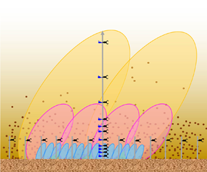
According to the Townsend's attached eddy hypothesis (shown as the schematic in figure 4), the flow in the logarithmic layer is filled with wall-attached eddies. Here, the velocity is defined as the sum of the attached-eddy-induced velocity increments (Yang et al. Reference Yang, Baidya, Johnson, Marusic and Meneveau2017; Xie et al. Reference Xie, de Silva, Baidya, Yang and Hu2021), i.e.

(5.3)\begin{equation} u(z) = \sum_{i = 1}^{N_{z}} a_{i}, \end{equation}

where $u(z)$ is the instantaneous streamwise fluctuation at a distance $z$ from the wall in the logarithmic layer, $a_{i}$ is the $\delta /2^{i}$-sized attached-eddy-induced streamwise velocity. The number of wall-attached eddies that contribute to $u(z)$ equals the integral from $z$ to $\delta$ of the eddy population density $P(z)$; that is, $N_{z}=\int _{z}^{\delta } P(z) \,\textrm {d} z$. Because the sizes of the wall-attached eddies scale as their distances from the wall, $P(z)$ is inversely proportional to the distances from the wall $z$, i.e. $P(z) \sim 1 / z$.

Figure 4. A schematic of the attached eddies. The two points are at a distance $z$ from the wall and are displaced by a distance $r$ in the streamwise direction.

The streamwise velocity difference between two points with distance $r$ is written as

(5.4)\begin{equation} u(x, z)-u(x+r, z) = \sum_{i = 1}^{N_{z}}\left(a_{i}-a_{i}^{\prime}\right)\!. \end{equation}

A large-scale attached eddy (coloured yellow in figure 4) contributes the same increment to both the two points and a small-scale attached eddy (coloured blue in figure 4) contributes to neither. Thus, the velocity difference with distance $r$ only contains contributions from intermediate-sized eddies (coloured carmine in figure 4)

(5.5)\begin{equation} u(x, z)-u(x+r, z) = \sum_{i = N_{r}}^{N_{z}}\left(a_{i}-a_{i}^{\prime}\right),\quad N_{r} \sim \ln (\delta / r), \end{equation}

where $N_r$ is the number of wall-attached eddies that contribute to $u(z)$ but their size less than $r$. Then, a logarithmic scaling of the second-order structure function can be obtained by squaring both sides of (5.5) and taking the ensemble average

(5.6)$$\begin{gather} \left\langle[u(x, z)-u(x+r, z)]^{2}\right\rangle \sim\left(N_{z}-N_{r}\right)\left(\left\langle a_{i}^{2}\right\rangle+\left\langle a_{i}^{\prime 2}\right\rangle-2\left\langle a_{i} a_{i}^{\prime}\right\rangle\right)\nonumber\\ \sim\left(N_{z}-N_{r}\right)\big(\big\langle a^{2}\big\rangle-\left\langle a a^{\prime}\right\rangle\big) \sim N_{z}-N_{r} \sim \ln (r / z); \end{gather}$$

that is

(5.7)\begin{equation} \left\langle[u(x, z)-u(x+r, z)]^{2}\right\rangle = A+B \ln (r / z). \end{equation}

In addition, the derivative of the second-order structure function,

(5.8)\begin{equation} {\rm d} S_{2, u}(r / z) / {\rm d}(r / z) = B \frac{1}{r / z}, \end{equation}

plays the role of an energy density. The pre-multiplied derivative of the second-order structure function is equal to the parameter $B$; that is

(5.9)\begin{equation} \frac{r}{z} \,{\rm d} S_{2, u}(r / z) / {\rm d}(r / z) = B, \end{equation}

which is a measure of the kinetic energy of eddies of size $r$.

Figure 5(a) presents the second-order structure functions of streamwise velocity fluctuations in different stages of the sandstorm, where black lines represent the theoretical formulas based on stationary atmospheric turbulence (de Silva et al. Reference de Silva, Marusic, Woodcock and Meneveau2015; Chamecki et al. Reference Chamecki, Dias, Salesky and Pan2017; Xie et al. Reference Xie, de Silva, Baidya, Yang and Hu2021). The inset plotted results in log–log scales to better assess the power-law behaviour. There are significant differences in the profiles of the structure function among the different stages. In the steady stage, the profile agrees well with the theoretical formulas of the log–linear law in the energy-containing region and the two-thirds power law in the inertial region. However, in the rising and declining stages, the profiles deviate from the theoretical formula, and the degree of deviation in the energy-containing region becomes increasingly significant with increasing structural scale. This may imply that the existing formula based on stationary atmospheric flows is not suitable for scaling the cumulative energy of eddies on different scales in the non-stationary process of the sandstorm. Although the profiles in non-stationary cases are different from the existing formula, there are still intervals following the predicted log–linear behaviour and two-thirds power law. In the inertial subrange ($r/z < 1$), as shown by the inset in figure 5(a), the profiles of the second-order structure function in log–log scales at different stages are straight, implying a power law. The power-law exponents for the three stages are $p = 0.68 \pm 0.04$, $0.66 \pm 0.05$ and $0.66 \pm 0.04$ by fitting the data, which are in general agreement with $p = 2/3$ predicted by the Kolmogorov's two-thirds law (Frisch & Kolmogorov Reference Frisch and Kolmogorov1995), and also match $p = 0.68$ for the ASL, $p = 0.67$ for a laboratory result (de Silva et al. Reference de Silva, Marusic, Woodcock and Meneveau2015) and $p = 0.68 \pm 0.01$ for the Rayleigh–Bénard convection (Sun, Zhou & Xia Reference Sun, Zhou and Xia2006). However, in the energy-containing region ($z < r \ll \delta$), the parameter $B$ that represents how quickly the cumulative TKE increases with increasing scale (Townsend Reference Townsend1976; Falkovich Reference Falkovich2018) is changed (as shown in figure 5b), where $B$ is obtained from the pre-multiplied derivative of the second-order structure function. Figure 5(b) shows that the pre-multiplied derivatives of the second-order structure function (a measure of the kinetic energy of eddies with scale $r$, Davidson et al. Reference Davidson, Krogstad and Nickels2006a) vs the streamwise length $r/z$ exhibit a plateau at all three stages of the sandstorm, but there are significant differences in the range (representing the interval of the logarithmic law) and magnitude (i.e. the value of $B$) of the plateau.

Figure 5. (a) Plots of the second-order structure function of the streamwise velocity fluctuations $\langle \Delta u^{2+}\rangle$, the inset shows the results at a log–log scale; (b) the corresponding pre-multiplied derivative $(r / z)[\textrm {d}\langle \Delta u^{2+}\rangle / \textrm {d}(r / z)]$ vs $r/z$ in the rising (red line), steady (blue line) and declining (green line) stages of the sandstorm at a 5 m height, where the plateau magnitude is the value of $B$, ‘$+$’ denotes the inner scaling, $u^{2+}=u^{2} / u_{\tau }^{2}$, $\langle {\cdot } \rangle$ denotes the time average, black lines represent the theoretical formulas based on the stationary atmospheric flow, $B = 4/3\kappa ^{-2/3} \approx 2.5$ (Chamecki et al. Reference Chamecki, Dias, Salesky and Pan2017; Xie et al. Reference Xie, de Silva, Baidya, Yang and Hu2021), $A = 2.95$ and $M_{p} = 3.12$ (de Silva et al. Reference de Silva, Marusic, Woodcock and Meneveau2015). The illustration shows the evolution of $B$ obtained from the plateau value over time. See figure 15 in Appendix B for the results of another sandstorm.

The plateau range moves left from larger scales of approximately $z \ll r < \delta$ at the right side in the rising stage to $z < r \ll \delta$ in the steady and declining stages, while the plateau magnitude decreases from $B = 23.3$ to 2.8 and then increases slightly to 4.8. These changes suggest that in the rising stage of the sandstorm, in addition to the larger size of the energetic structure, the kinetic energy is also stronger because the scales of the convective structures dominated by thermal turbulence are larger and the energy is mainly concentrated in the larger energetic structures. In the steady stage, both the scale and the kinetic energy decrease. This is because shear-driven turbulence is dominant in this case, and the strong shear not only acts on the surface to generate a new small-scale vortex but also breaks up the large convective structure (Hunt & Morrison Reference Hunt and Morrison2000; Liu et al. Reference Liu, Shi and Zheng2022), transferring energy to the small scales and thus reducing the kinetic energy of the energetic structures. Especially in the declining stage, the kinetic energy of the energetic structures is slightly enhanced again, although the further length scale decreases. This may be plausible given that the attenuated shear turbulence, especially suppressed by gravity when stably stratified, is unable to generate more small-scale vortices, so that the larger-scale structures cannot retain their coherence, resulting in a scale reduction and refocusing of the energy on these energetic structures due to the absence of small scales.

Specifically, the evolution of the scaling parameter $B$ over time in the inset of figure 5(b) shows that $B$ decreases rapidly in the rising stage of the sandstorm, remains virtually unchanged in the steady stage and increases slightly in the declining stage. This indicates that the cumulative TKE increases more quickly with increasing scale in the non-stationary stage of the sandstorm than in the stationary stage, even in the declining stage where the velocity attenuates. Given that $B = 2.8$ in stationary sandstorm flows is close to $B = 2.35{-}3$ in high-Reynolds-number ASL (de Silva et al. Reference de Silva, Marusic, Woodcock and Meneveau2015; Chamecki et al. Reference Chamecki, Dias, Salesky and Pan2017) and $B = 2.5$ in laboratory TBL (Davidson et al. Reference Davidson, Krogstad and Nickels2006a,Reference Davidson, Nickels and Krogstadb; de Silva et al. Reference de Silva, Marusic, Woodcock and Meneveau2015) and channel (Katul et al. Reference Katul, Ghannam, Bou-Zeid, Gerken and Chamecki2018; Xie et al. Reference Xie, de Silva, Baidya, Yang and Hu2021) flows at low and moderate Reynolds numbers, it is inferred that the parameter $B$ should be independent of the Reynolds number. This is consistent with the conclusion of de Silva et al. (Reference de Silva, Marusic, Woodcock and Meneveau2015) using datasets that span several orders of magnitude in Reynolds number, up to $Re_\tau \sim O(10^6)$. Therefore, it is not the Reynolds number, but rather the variability in multiple factors (dust concentration, thermal stability and flow acceleration) during the sandstorm that is responsible for the increase in $B$, that is, the more rapid increase in the cumulative TKE with increasing scale.

Sandstorms as a typical wind-blown-sand two-phase flow, the effect of particles on turbulence during sandstorms needs to be considered because the sand concentration changes dramatically. Therefore, figure 6(a) presents the resulting $B$ at various PM10 concentrations $\bar {C}$. In the sandstorm steady stage with small $B$, where the acceleration and thermal stability close to zero, $B$ remains almost constant even if $\bar {C}$ varies by an order of magnitude. This indicates that the cumulative TKE scaling law in the energy-containing region is only minimally affected by sand particles in the sandstorm. In the early rising stage, where $\bar {C}$ is close to zero, $B$ changes across an order of magnitude, indicating that the flow acceleration and thermal stability may be the factors contributing to the change in $B$.

Figure 6. Variations in parameter $B$ of the logarithmic scaling law with the (a) average PM10 dust concentration $\bar {C}$ at different heights, (b) acceleration $a$ of the incoming flow and (c) thermal stability parameter $z/L$ during the sandstorm. See figure 16 in Appendix B for the results of another sandstorm.

As shown in figure 1(a), in the rising stage, the velocity is increasing and the flow acceleration has a positive value because the local atmosphere gains energy from the cold air mass brought by the cold front. The exhaustion of the energy brought by the cold air mass leads to the reduced wind velocity and flow deceleration in the declining stage. The accelerated flow has previously been confirmed to be a key factor governing turbulence properties. The flow acceleration significantly enhances the near-wall Reynolds shear stresses (Fernholz & Waenack Reference Fernholz and Waenack1998; Piomelli, Balaras & Pascarelli Reference Piomelli, Balaras and Pascarelli2000; Joshi, Liu & Katz Reference Joshi, Liu and Katz2011; Piomelli & Yuan Reference Piomelli and Yuan2013), making the large-scale coherent structures more elongated (Talamelli et al. Reference Talamelli, Fornaciari, Westin and Alfredsson2002). The flow acceleration also reduces the burst frequency (Kline et al. Reference Kline, Reynolds, Schraub and Runstadler1967; Ichimiya, Nakamura & Yamashita Reference Ichimiya, Nakamura and Yamashita1998; Bourassa & Thomas Reference Bourassa and Thomas2009) and thus the number of near-wall cycles (Piomelli et al. Reference Piomelli, Balaras and Pascarelli2000; Joshi et al. Reference Joshi, Liu and Katz2011). Additionally, the acceleration process affects the Kármán constant (Emadzadeh, Chiew & Afzalimehr Reference Emadzadeh, Chiew and Afzalimehr2010; Joshi et al. Reference Joshi, Liu and Katz2011), enhances the turbulence anisotropy (Jung & Chung Reference Jung and Chung2012) and increases the transition Reynolds number (Costantini et al. Reference Costantini, Hein, Henne, Klein, Koch, Schojda, Ondrus and Schröder2016). Therefore, to explore the effects of flow acceleration on the logarithmic scaling law of the second-order structure function, figure 6(b) shows the variation in $B$ with the flow acceleration (denoted as $a$) during the sandstorm process. The flow acceleration $a$ represents the changing rate of mean wind velocity and is defined as $a = \textrm {d}U/\textrm {d}t$. Here, $a$ is estimated from the average changing rate of velocity in the time-varying mean wind flow extracted by EMD in each segment obtained by the adaptive segmentation method. The magnitude of $a$ represents how quickly the sandstorm develops from the beginning to the steady stage and from the steady stage to its end. In addition, the flow acceleration indicates the amount of kinetic energy gain from the local synoptic system (such as, cold air mass) during the rising stage. The value of $a$ (${\sim }O(10^{-3})$) involved in this study, while seemingly small, represents the development time from the beginning ($0\,\textrm {m}\,\textrm {s}^{-1}$) to the steady stage (10–15 m s$^{-1}$) of a sandstorm in real nature, which is approximately 3–5 h (approximately 90 % of all 79 sandstorm events with long-term observation), being more rapid than the development time (9 h) of typhoons recorded by Wang et al. (Reference Wang, Wu, Tao, Li and Kareem2016). The overall trend in figure 6(b) suggests an increasingly significant increase in $B$ with $a$, i.e. $B$ remains unchanged when $a$ is small, whereas the increase in $B$ with $a$ is pronounced at a large value of $a$. This indicates that the violent acceleration of the flow field changes the energy distribution of the multiscale structures and concentrates the TKE in large-scale energetic structures. Note that the profiles of $B$ varying with $a$ are not well collapsed. This is because the rising stage is accompanied by changes in thermal stability in addition to acceleration.

Therefore, figure 6(c) plots the change in $B$ vs the Monin–Obukhov stability parameter $z/L$ for all of the sandstorm data. As expected, the variation in $B$ with $z/L$ is systematic, suggesting that thermal stability is also a key parameter affecting the TKE of energetic structures. Under the near-neutral stratified condition with $z/L$ close to zero, the significant change in $B$ is caused by the incoming flow that still dramatically changes when $z/L$ decreases rapidly to near zero in the rising stage. In the unstable stratified regime with negative $z/L$, $B$ increases with decreasing stability. This indicates that affected by thermal instability, the kinetic energy of eddies in the energy-containing region is enhanced.

Figure 6 suggests that the turbulent properties are potentially affected by thermal stratification, suspended particles and flow acceleration. However, the three factors vary simultaneously. To disentangle the various effects in a field study, more datasets from long-term observations were selected where only one parameter is different but other parameters are similar, and the results are shown in figure 7. The results obtained from the laboratory experiments (Davidson et al. Reference Davidson, Krogstad and Nickels2006a,Reference Davidson, Nickels and Krogstadb; de Silva et al. Reference de Silva, Marusic, Woodcock and Meneveau2015), the ASL observations (de Silva et al. Reference de Silva, Marusic, Woodcock and Meneveau2015; Chamecki et al. Reference Chamecki, Dias, Salesky and Pan2017; Katul et al. Reference Katul, Ghannam, Bou-Zeid, Gerken and Chamecki2018) and theoretical formulas (Chamecki et al. Reference Chamecki, Dias, Salesky and Pan2017; Xie et al. Reference Xie, de Silva, Baidya, Yang and Hu2021) are also included in figure 7 for comparison. Figure 7(a) considers the effect of only the PM10 dust concentration on parameter $B$ based on datasets in near-neutral ASLs with steady wind. Although the current ASL results (shown as diamonds) are not well converged (the scatter would be smaller in a controlled laboratory experiment), the overall trend indicates that the parameter $B$ does not change significantly with PM10 concentration $\bar {C}$ and is generally consistent with the existing laboratory and ASL results. In addition, all of these experimental data fluctuate around the theoretical result shown by the red dashed line. It is predictable that the parameter $B$ does not change with $\bar {C}$ when the mass loading ($\varPhi _{m}$) is smaller than $7.78 \times 10^{-4}$ (corresponding average PM10 dust concentration of 1.96 mg m$^{-3}$). This condition belongs to the one-way coupling sparse two-phase flow ($\varPhi _m < 10^{-3}$) suggested by Elghobashi (Reference Elghobashi1994), Balachandar & Eaton (Reference Balachandar and Eaton2010) and Brandt & Coletti (Reference Brandt and Coletti2022), where the particle effects on turbulence are negligible. The result in figure 7(a) may provide support for the conclusion obtained from figure 6(a).

Figure 7. The effect on parameter $B$ by the (a) average PM10 dust concentration $\bar {C}$; (b) acceleration $a$ of the incoming flow, where black solid circles denote the results of accelerating incoming flow and hollow circles are the results of decelerating incoming flow, and the red solid line is the fitting curve for acceleration $a > 0$; and(c) thermal stability parameter $z/L$, where black and blue squares are the results of unstable and stable surface-layer data, respectively. The black and blue dashed lines are the corresponding fitted curves. In all panels, the red dashed line represents the theoretical formulas based on the stationary atmospheric flow, $B = 4/3\kappa ^{-2/3} \approx 2.5$ (Chamecki et al. Reference Chamecki, Dias, Salesky and Pan2017; Xie et al. Reference Xie, de Silva, Baidya, Yang and Hu2021), the red asterisks are the laboratory (LAB) results from Davidson et al. (Reference Davidson, Krogstad and Nickels2006a,Reference Davidson, Nickels and Krogstadb), de Silva et al. (Reference de Silva, Marusic, Woodcock and Meneveau2015) and Chung et al. (Reference Chung, Marusic, Monty, Vallikivi and Smits2015) and the carmine stars are the ASL results from de Silva et al. (Reference de Silva, Marusic, Woodcock and Meneveau2015), Chamecki et al. (Reference Chamecki, Dias, Salesky and Pan2017) and Katul et al. (Reference Katul, Ghannam, Bou-Zeid, Gerken and Chamecki2018).

Figure 7(b) plots the individual effect of flow acceleration on the parameter $B$ based on datasets in near-neutral sand-free ASL flows. The results of accelerating and decelerating incoming flow are shown by black solid and hollow circles, respectively. As shown by the black solid circles, the effect is remarkable when the velocity is increasing (with a positive acceleration $a$); that is, the parameter $B$ increases with increasing $a$. A parametric equation is fitted to the exponential trend of accelerated flow data to model the variation in $B$ with $a$ and is given as,

(5.10)\begin{equation} B = B_{0}+0.06\exp (3180 a),\quad a\ge 0, \end{equation}

where $B_{0} = 2.5$ is the theoretical result. When the flow is stationary (with an acceleration of $a = 0$), the functional form of the fitted equation (5.10) approaches the invariant value of the parameter $B$ and is consistent with the existing results, while it depicts an increasing $B$ at high $a$. It is well known that the increase in wind velocity is attributed to the local atmospheric system gaining energy from the environment. Energy cascade theory (Richardson Reference Richardson1922) suggests that large-scale turbulence structures transfer kinetic energy gained from the mean flow field to small-scale turbulence structures, and the bispectrum analysis during sandstorm by Liu et al. (Reference Liu, Shi and Zheng2022) suggested that large-scale coherent structures gain energy from nonlinear interactions in the rising stage. Therefore, a higher acceleration $a$ indicates that large-scale turbulence structures in the local atmospheric system gain more kinetic energy from the mean flow field, which leads to an increase in $B$ because it is a measure of the kinetic energy of large structures in the energy-containing region. Meanwhile, flow acceleration increases the Reynolds shear stress at the near-wall surface (Piomelli et al. Reference Piomelli, Balaras and Pascarelli2000; Joshi et al. Reference Joshi, Liu and Katz2011), resulting in an increase in the velocity gradient and thus the streamwise spacing between different hairpin vortices in the hairpin vortex packet that form the large-scale coherent structure, consequently increasing the scale of the large-scale structure (Adrian et al. Reference Adrian, Meinhart and Tomkins2000; Volino Reference Volino2020). This provided evidence supporting the larger size of the energetic structure in the rising stage of the sandstorm shown in figure 5(b). However, for negative acceleration $a$, the effect of decelerated flow on parameter $B$ is not significant, as shown by the hollow circles in figure 7(b).

The effect of stratification stability on the parameter $B$ is shown in figure 7(c) based on sand-free ASL flows with steady wind. As expected, the parameter $B$ increases with decreasing stability (increasing $-z/L$), and the variation follows an approximately linear increase in the unstable regime, as shown by black squares. Under stable conditions, a few cases show a slight linear increase in the parameter $B$ with increasing stability, as shown by blue squares. In the near-neutral ASL, the parameter $B$ results agree well with the existing results shown by red asterisks, carmine stars and red dashed lines in figure 7(c). The linear trend is fitted by an empirical correlation to model the variation in the parameter $B$ with $z/L$ and is given as

(5.11)\begin{equation} B = \left\{\begin{array}{@{}ll@{}} B_{0}+1.03 z / L, & z / L \geq 0, \\ B_{0}-9.42 z / L, & z / L<0. \end{array}\right. \end{equation}

The self-organized state of multiscale turbulent structures shows a stronger response to unstable conditions than to the stable conditions. A probable interpretation is that buoyant currents shred the synoptic-scale structures into large turbulence structures and further break those structures into small-scale structures (Hunt & Morrison Reference Hunt and Morrison2000; Lotfy et al. Reference Lotfy, Abbas, Zaki and Harun2019; Liu et al. Reference Liu, Shi and Zheng2022), which may cause the energy of large-scale structures to be more significant, that is, the cumulative TKE increases more rapidly with increasing scale in the energy-containing region. The enhanced energy fraction of large-scale structures under unstable conditions is also observed in other ASL measurements and numerical simulations (Kaimal et al. Reference Kaimal, Wyngaard, Izumi and Coté1972; Feigenwinter, Vogt & Parlow Reference Feigenwinter, Vogt and Parlow1999; Kim & Park Reference Kim and Park2003; Salesky et al. Reference Salesky, Katul and Chamecki2013; Banerjee et al. Reference Banerjee, Katul, Salesky and Chamecki2015; Lotfy et al. Reference Lotfy, Abbas, Zaki and Harun2019; Brilouet et al. Reference Brilouet, Durand, Canut and Fourrié2020; Liu et al. Reference Liu, Shi and Zheng2022). The slight increase in the parameter $B$ in stably stratified ASLs indicates a focus of energy in the energetic structures, although the turbulence is suppressed by stable thermal conditions, providing further evidence supporting the results in figure 5(b).

6. Concluding remarks

Turbulence fluctuating data are extracted from the velocity time series over the entire sandstorm process by removing the time-varying mean flow with EMD and then the adaptive segmented processing is employed to ensure stationarity and statistical convergence. Statistical analyses of these turbulence signals indicate that thermal turbulence and shear turbulence exhibit a competitive evolutionary process in the rising and declining stages of the sandstorm due to the non-stationarity of sand-laden atmospheric turbulence. That is, the driving factor transitions from the dominant thermal turbulence in the rising stage to the weakened thermal turbulence and dominant shear turbulence in the steady stage and then to the suppressed turbulence motion in the declining stage due to the enhanced thermal stability.

With the evolution of this driving factor, the self-organized state of multiscale structures in the energy-containing region of the sand-laden turbulence also changes significantly as the sandstorm evolves. The logarithmic scaling law of cumulative TKE in the non-stationary rising and declining stages differs significantly from the existing theoretical results. The growth rate of the cumulative TKE in non-stationary stages is much higher than that in the middle stage of sandstorms with steady flow, and the scale of the energetic structures is larger in the rising stage and shorter in the declining stage. This suggests that the structural characteristics in the sandstorm process undergo an evolutionary process: at the beginning the sandstorm, the energy is mainly concentrated in larger energetic structures. Later on, as the sandstorm develops, the scale and kinetic energy of these structures is reduced because energy is transferred to smaller-scale vortices generated by strong shear. Eventually, at the end of the sandstorm, the energy re-focus on the shorter energetic structure because the suppressed shear leads to discontinuation of the generation of small-scale vortices and the difficulty in maintaining large-scale vortices.

By investigating the effects of independent environmental factors, it is found that the increase in the rate of increase in the cumulative TKE in the rising stage of the sandstorm is mainly caused by the flow acceleration (non-stationarity of the flow) and thermal instability, while it is due to the stable stratification in the declining stage. The influence of PM10 particles is negligible throughout the sandstorm process.