


1. Introduction
Because weather is a direct input to the biological process of plant growth, agriculture has been the focus of many studies of climate impacts on crop yield production. Two primary approaches to research on the relationship between weather/climate and agriculture have been the Ricardian approach and estimation of crop yield response functions. These two approaches are based on the common functional relation Footnote 1 :
 $$y=f\left(H,P,S,L\right),$$
where y is the agriculturally relevant measure of interest, H is heat exposure, P is total precipitation, S is soil characteristics, and L is other nonweather factors such as input mix, technology, or other human factors. If the dependent variable is farmland value as a function of climate (the multiyear average, or distribution, of weather), then the estimation of Equation (1) is called the Ricardian approach; if y = crop yield as a function of weather, then Equation (1) is the crop yield response function.
Mendelsohn et al. (Reference Mendelsohn, Nordhaus and Shaw.1994) introduced the Ricardian approach to study temperature impacts on agriculture. As summarized in Ortiz-Bobea (Reference Ortiz-Bobea2020), various theoretical and empirical extensions of climate change impacts on agriculture through the Ricardian approach have been studied. Schlenker and Roberts (Reference Schlenker and Roberts.2009) first popularized heat exposure bins to study nonlinear temperature effects on crop yields. Deschênes and Greenstone (Reference Deschênes and Greenstone.2007) suggested the panel estimation approach to scrutinize the relationship between random weather fluctuation and agricultural output. Many econometric models of climate change and weather impacts on agricultural yields have followed Fisher et al.’s (Reference Fisher, Hannemann, Roberts and Schlenker.2012) discussion of Deschênes and Greenstone (Reference Deschênes and Greenstone.2007, Reference Deschênes and Greenstone.2012) along both theoretical and empirical lines. In empirical applications, Tack et al. (Reference Tack, Harri and Coble.2012) studied the higher moments of yield responses and Tack et al. (Reference Tack, Coble and Barnett.2018) analyzed their implications on crop insurance. Belasco et al. (Reference Belasco, Cooper and Smith.2020) investigated the potential of a weather-based crop disaster program. Goodwin and Piggott (Reference Goodwin and Piggott.2020) analyzed weather and technology interactions in crop insurance and Le et al. (Reference Le, Jeffrey and An.2020) studied weather impacts on the dairy sector.
As geospatially referenced and gridded data have become readily available, significant effort has been devoted to econometric analysis of weather impacts on agriculture through crop yield response functions and so-called Ricardian models of land value. Dell et al. (Reference Dell, Jones and Olken.2014) summarized these efforts as econometric identification and specifications of nonlinearity, causality, and estimation of a yield damage function in response to weather and climate. Accordingly, Auffhammer et al. (Reference Auffhammer, Hsiang, Schlenker and Sobel.2013) pointed out five major econometric pitfalls associated with weather data and climate model output in economic analysis: the choice of weather data set, averaging station-level data across space, correlation between weather variables, endogenous weather data coverage, and spatial correlation. While the first four pitfalls can be handled by proper data management or are addressed in the previous literature, spatial correlation that can be rigorously managed using spatial econometric techniques has received less attention in the Ricardian and yield response threads of the literature.
In the Ricardian approaches, spatial error structure was adopted from earlier literature (Schlenker et al., Reference Schlenker, Hanemann and Fisher.2006). Baylis et al. (Reference Baylis, Paulson and Piras.2011) numerically explored the spatial dependence structure in error and dependent variables with fixed and random effects (RE) panel regressions. Dall’erba and Dominguez (Reference Dall’erva and Dominguez.2016) applied the spatial lag of weather variables in the Ricardian panel regression. Those studies, however, focused on the calculation of the direct and indirect marginal effects of weather variables or the possibility of performing spatial econometric panel regression. To the best of our knowledge, there is not any detailed discussion of the source of spatial correlation, pros and cons of alternative model specifications, and prediction performance comparisons in this literature. The crop yield response function literature has even fewer applications of spatial econometrics in panel regressions. Given that the crop yield response function is most often the base analysis in the areas of climate change, food security, nutrition, and development economics, the lack of studies using or evaluating spatial econometric models of crop yield response is quite surprising. Footnote 2 There has been great interest in using spatial econometric models of crop yield response in precision agriculture research (e.g., Anselin et al., Reference Anselin, Bongiovanni and Lowenberg-DeBoer.2004; Liu et al., Reference Liu, Griffin, Kirkpatrick and Monfort.2015). The data used in these studies, however, are limited and do not go beyond cross-sectional analysis of prediction performance.
When ignoring or not properly incorporating spatial correlation in crop yield response functions, four unintended econometric issues could arise in general. First, an improper model specification could be applied. Given that the true crop yield response function data generating process is unknown, spatial correlation may be present for various reasons. Since the specification strategies in spatial econometrics are dependent upon the source of spatial correlation, the choice of spatial econometric models could be misguided. Second, estimated coefficients could be biased due to measurement error. If a spatial correlation is caused by measurement error or omitted variables, a proper spatial econometric model is one of the possible remedies (LeSage and Pace, Reference LeSage and Pace.2009). Because proper instrumental variables or control functions are not available in many cases, the use of a spatial econometric model for crop yield response is a feasible alternative. Third, statistical inference of estimates could be imprecise. If a spatial correlation is local, that is, exists in error terms, the estimates could be unbiased, but inference based on these estimates could be imprecise. Last, there is no theoretical standard or ad hoc guidance for whether the spatial econometric models in the previous literature are properly adopted in practice.
To fill this gap, this study addresses the question of how spatial correlation can be presented and specified using spatial econometrics to model the crop yield response function. To specify alternative models, we first delve into the source of spatial correlation that gives rise to the necessity of using spatial econometrics and motivates the need for this study. Three major sources of spatial correlations this study identifies are spatial data aggregation processes, omitted variables, and spatial heterogeneity. We initially select seven competing models that are the most frequently adopted functional forms in the literature. Additionally, we replicate these models with the nonlinear temperature bins used in Schlenker and Roberts (Reference Schlenker and Roberts.2009). In total, we compare the prediction performance of 14 different model specifications. The comparison analysis in this study is focused on better prediction capability rather than better coefficient estimates. This is because the true data generating process of equation (1) that relates crop yields to spatially varying components remains unknown. Besides, making predictions is one of the primary purposes of research applying crop yield response functions, especially in the context of climate change impacts on agriculture. This also helps to avoid the unresolved controversial debate on identification and specification in spatial econometrics models provoked by Gibbons and Overman (Reference Gibbons and Overman.2012) and Pinkse and Slade (Reference Pinkse and Slade.2010).
The data used in the performance comparisons are county-level corn yields, temperature, total precipitation, and soil characteristics in the US from 1981 to 2018. Spatially gridded weather and soil data were aggregated up to counties. Due to the intensively managed nature of irrigated crops that masks the impact of precipitation on yield, we limit our study counties to those east of the 100th Meridian line as in Schlenker and Roberts (Reference Schlenker and Roberts.2009). The prediction capabilities of candidate models are compared using in-sample prediction standards. We also perform out-of-sample predictions for 2013–2018 using the coefficient estimates based on 1981–2012 data. Year-stratified bootstrapping is also implemented to statistically test prediction performance using the 1981–2012 data.
2. Spatial Econometric Models of Crop Yield Response
2.1. NonSpatial Panel Regression
A general crop yield response function specifying the relationships in Equation (1) can be presented as the panel regression equation:
 $${y_{it}} = g\left( {{\textbf{h}_{it}}; \beta } \right) + {\delta _1}{P_{it}} + {\delta _2}P_{it}^2 + {\tau _1}t + {\tau _2}{t^2} + {\mu _i} + {\varepsilon _{it}},$$
where g(⋅) is a nonlinear function of heat units, h it , with the response coefficients β , the second and third terms are a quadratic precipitation equation with the response coefficients δ, μ i is the individual (county) fixed effect (FE), t is the time trend, τ is its coefficient, and ϵ it is the random error. Roberts et al. (Reference Roberts, Schlenker and Eyer.2013) empirically showed that the quadratic form in precipitation achieves sufficient model fit. To control for advances in technology and other time-dependent trends, the quadratic specification of time trend instead of time FE has generally been used in the literature (Miao et al., Reference Miao, Khanna and Huang.2016; Schlenker and Roberts, Reference Schlenker and Roberts.2009). This study follows the prior literature and adopts a quadratic function of the total precipitation and time trend variables Footnote 3 in all model specifications that follow.
Based on agronomic knowledge, corn yield is dependent upon heat accumulation rather than temperature measures (e.g., mean, maximum, and minimum temperature) alone (Baskerville and Emin, Reference Baskerville and Emin.1969). The total amount of heat exposure measured in degree days during the growing season (growing season degree days: GDDs) is a popular measure of heat contribution to crop development in crop yield response function or Ricardian approaches (Schlenker et al., Reference Schlenker, Hanemann and Fisher.2006; Schlenker and Roberts, Reference Schlenker and Roberts.2009). Following Baylis et al. (Reference Baylis, Paulson and Piras.2011) and Schlenker et al. (Reference Schlenker, Hanemann and Fisher.2006), this study adopts the quadratic form of GDDs over the range 8–32°C for the crop development and the square root of extreme heat GDDs (above 34°C) to capture excessive heat impacts. Additionally, we replicate the Chebyshev polynomial specification of GDD bins used in Schlenker and Roberts (Reference Schlenker and Roberts.2009), as discussed in Section 2.5.
For notational simplicity, we suppose
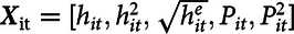 $${\textbf{X}_{{\rm{it}}}} = [{h_{it}},h_{it}^2,\sqrt {h_{it}^e} ,{P_{it}},P_{it}^2]$$
is a vector containing the quadratic form of GDDs, square root of extreme heat GDDs, h
it
e
, and the quadratic form of total growing season precipitation. The corresponding response coefficients are
β
= [β
1,β
2,β
3,δ
1,δ
2]. The Pooled regression specification can be presented as:
$${\textbf{X}_{{\rm{it}}}} = [{h_{it}},h_{it}^2,\sqrt {h_{it}^e} ,{P_{it}},P_{it}^2]$$
is a vector containing the quadratic form of GDDs, square root of extreme heat GDDs, h
it
e
, and the quadratic form of total growing season precipitation. The corresponding response coefficients are
β
= [β
1,β
2,β
3,δ
1,δ
2]. The Pooled regression specification can be presented as:
 $$y_{it}={\textbf{X}}_{it} \beta +\tau _{1}t+\tau _{2}t^{2}+\varepsilon _{it}.$$
Soil characteristics (S) is only component in Equation (1) missing in Equation (3). As Yun and Gramig (Reference Yun and Gramig.2019) pointed out, soil characteristics influence soil conditions that contribute to agricultural yields based on complex relationships. In most cases, time-varying soil variables (e.g., soil moisture level) are not available because of the implausibility of measurement. Generally available soil characteristics (e.g., soil water holding capacity) from the gridded Soil Survey Geographic Database (gSSURGO) are location-specific but not time-dependent variables. In both the crop yield response function and Ricardian approaches, the FE term μ i in (2) controls for time-invariant soil characteristics (among other things, as discussed below). The FE panel regression can be specified by altering Equation (3) as:
 $$y_{it}={\textbf{X}}_{it}\beta +\tau _{1}t+\tau _{2}t^{2}+\mu _{i}+\varepsilon _{it}.$$
Even though we include two important weather factors from Equation (1), some key weather variables affecting agricultural outputs like vapor pressure deficit (Lobell et al., Reference Lobell, Roberts, Schlenker, Braun, Little, Rejesus and Haemmer.2014) or other drought measures are not considered in Equation (4). We would, of course, prefer to include omitted weather variables as control variables. They are, however, generally unavailable. The instrumental variables (IVs) or control function approaches can be used to overcome omitted variable bias. It is, however, challenging to find proper IVs because potential IVs are correlated with agricultural output. The panel specification in Equation (4) assumes weather variables are randomly and exogenously given, rendering past weather an improper IV or control factor. FE terms may control for unobserved heterogeneity. In practice, it is impossible to discern time-invariant soil factors from location-specific omitted weather variables. Auffhammer et al. (Reference Auffhammer, Hsiang, Schlenker and Sobel.2013) pointed out that the RE model can be used to address possible spatial correlation in the omitted weather variables. In spatial econometrics, the omitted variable is a well-studied motivation to model a spatial correlation structure in the regression error term (LeSage and Pace, Reference LeSage and Pace.2009). Keeping soil factors in the control variable set, therefore, the counterpart RE model to the FE model in Equation (4) is:
 $$y_{it}={\textbf{X}}_{it} \beta +\tau _{1}t+\tau _{2}t^{2}+{\textbf{S}}_{it}{\theta }+\varepsilon _{it},$$
where S it is a vector of soil characteristics Footnote 4 and θ contains the associated response coefficients.
2.2. Sources and Implications of Spatial Correlation
2.2.1. Spatial Aggregation in Weather
For a better description of the following model specifications, we estimate the county-level crop yield response function with the Parameter-elevation Relationship on Independent Slopes Model (PRISM) weather data, which is high resolution (4 × 4 km) grid cell data that is widely used throughout agricultural and applied economics. A PRISM grid cell is smaller than a county, and each county consists of a different number of grid cells. The right panel of Figure 1 generalizes an aggregation process of grid cell data to a county.
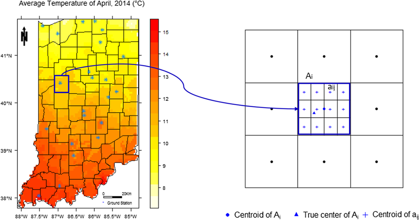
Figure 1. Spatial units of weather variable: average temperature in Indiana, USA, April 2014.
We can assume that there are regions A = A 1 ∪ A 2 ∪ ⋯ ∪ A n and A i ∩ A j = Ø for ∀i ≠ j. In a region A i , it consists of several subregions as A i = a i1 ∪ a i2 ∪ ⋯ ∪ a in i and a ir ∩ a is = Ø for ∀r ≠ s. In Figure 1, for example, A is the state of Indiana, A i is a County in Indiana, and a ij is a PRISM grid cell in county i. If the temperature of PRISM grid cell a ij is H ij and A i contains n i individual PRISM grid cells. Then, a grid cell’s temperature can be written as:
 $$H_{ij}=\overline{H}_{i}+v_{ij}=\sum _{j=1}^{n_{i}}w_{ij}H_{ij}+v_{ij},$$
where $\overline{H}_{i}$
is the county mean temperature (area-weighted by w
ij
) and v
ij
is a temperature variation from
$\overline{H}_{i}$
is the county mean temperature (area-weighted by w
ij
) and v
ij
is a temperature variation from $\overline{H}_{i}$
. From Equation (6), we have two propositions.
$\overline{H}_{i}$
. From Equation (6), we have two propositions.
Proposition 1: The larger the extent of spatial aggregation, the more spatial variation is lost, that is, spatial aggregation is a smoothing process such that as n
i
→ ∞, the absolute sum of v
ij
diverges, that is, $\lim _{n_{i}\rightarrow \infty } \sum _{j=1}^{n_{i}}|v_{ij}|$
is undefined.
$\lim _{n_{i}\rightarrow \infty } \sum _{j=1}^{n_{i}}|v_{ij}|$
is undefined.
Proposition 2: A larger spatial aggregation has less spatial correlation by Proposition 1. If k (e.g., State) is a larger geographic aggregation unit than that of i (e.g., county), then $\overline{H}_{k}$
is in [min(H
ij
),max(H
ij
)]. The spatial correlation (ρ) of two spatial units is ρ
k
≤ ρ
i
.
$\overline{H}_{k}$
is in [min(H
ij
),max(H
ij
)]. The spatial correlation (ρ) of two spatial units is ρ
k
≤ ρ
i
.
To empirically demonstrate these two propositions, we calculated Moran’s I statistic at the grid cell, county, and state for annual average temperature, GDDs, and total precipitation for March to August in Table 1 (full study period is available in Table S1 from Supplemental Materials) using the PRISM data.
Table 1. Moran’s I statistic of the yearly average temperature, growing season degree days (GDD) (March to August), total precipitation (March to August), and corn yields (bu/ac), 2001–2012
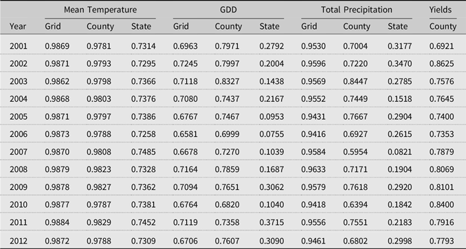
Note: The full table for 1981–2012 is available from Table S1 in the provided Supplemental Materials.
Table 1 generally meets Propositions 1 and 2. As the spatial extent of aggregation increases from grid cell (or county) to the entire state, spatial correlations tend to decline. Particularly, state-level spatial correlations are significantly lower than those of grid cells or counties for GDDs and total precipitation. Even though yearly temperature averages and GDDs both measure the magnitude of heat, GDDs exhibit a more significant reduction in state-level Moran’s I. From Table 1, we find that the reduced spatial variation (and spatial correlation) should pass through the error terms. County-level weather variables reveal a high-spatial correlation (relative to state-level) that is discussed in the next section in more detail.
The right panel of Figure 1 illustrates an additional proposition important to spatial correlation in the error terms. In the right panel of Figure 1, we suppose that the centroid of region A i (blue square) is the blue dot (●), and the unknown true center of the county is the blue triangle (▴). The most frequently adopted center of a spatial boundary is the centroid. The centroid is the physical center of mass over a spatial unit. There is, however, no evident reason why the centroid is the correct or best representative point for spatially varying quantities like weather variables.
Proposition 3: The true center of a spatial unit is not necessarily the centroid of the spatial unit. The most representative value of a weather variable for a given spatial unit, therefore, could be measured at any or many points within a spatial unit.
If we build a distance-based spatial weights matrix using the blue dot, the measurement error will go through the error terms again because errors are spatially correlated. From the above three propositions, we specify the spatial dependence structure in the error terms in the FE (Spatial Error Model (LeSage and Pace, Reference LeSage and Pace.2009), hereafter SEM) and RE (based on Kapoor, Kelejian & Prucha (Reference Kapoor, Kelejian and Prucha.2007), hereafter KKP) spatial models as:
 $$y_{it}={\textbf{X}}_{it} \beta+\tau _{1}t+\tau _{2}t^{2}+\mu _{i}+u_{it}, {\rm where} \, {\textbf{u}}_{N}={\rm r}\left({\textbf{I}}_{T}\otimes {\textbf{W}}_{N}\right){\textbf{u}}_{N}+{\varepsilon }_{N},$$
 $$y_{it}={\textbf{X}}_{it} \beta+\tau _{1}t+\tau _{2}t^{2}+{\textbf{S}}_{it}{\theta }+u_{it}, \rm \ where \,{\textbf{u}}_{N}={\rm r}\left({\textbf{I}}_{T}\otimes {\textbf{W}}_{\it{N}}\right){\textbf{u}}_{\it{N}}+{\varepsilon }_{\it N}$$
In Equations (7) and (8), the error structure is defined as u N = r( I T ⊗ W N ) u N + ϵ N , where N is the number of spatial observations, T is the length of time, r is the spatial error coefficient, I is an identity matrix, W is the spatial weights matrix, and ⊗ is the Kronecker product.
2.2.2. Spatial Correlation in Weather
It is widely noted that weather variables exhibit spatial correlation (Auffhammer et al., Reference Auffhammer, Hsiang, Schlenker and Sobel.2013; Dell et al., Reference Dell, Jones and Olken.2014). The previous literature of the Ricardian approaches motivated the use of spatial lags on weather variables by their spatial correlation (Baylis et al., Reference Baylis, Paulson and Piras.2011; Dall’erba and Dominguez, Reference Dall’erva and Dominguez.2016). Auffhammer et al. (Reference Auffhammer, Hsiang, Schlenker and Sobel.2013) stated that the spatial dependence of the regressors would not be a problem if the model correctly accounts for all weather variables. Spatial econometricians, however, certainly disagree with this argument (Anselin, Reference Anselin2006). A spatial correlation also could be an issue depending upon the spatial unit or the measurement of variables shown in Table 1. The model specification that accounts for spatially correlated weather variables is the spatial lagged X model (SLX) in Elhorst (Reference Elhorst2014):
 $$y_{it}={\textbf{X}}_{it}{\beta }+{\textbf{w}}_{i}{\textbf{X}}_{it}{\gamma} +\tau _{1}t+\tau _{2}t^{2}+\mu _{i}+\varepsilon _{it},$$
where γ is the spatial lag coefficient and w i is the ith row of the spatial weights matrix W .
2.2.3. Spatial Correlation in Crop Yields
In the general crop yield response function of Equation (2), an essential assumption of the panel regression is that observed crop choices are optimal and do not change (Deschênes and Greenstone, Reference Deschênes and Greenstone.2007). Since crop choice is the optimized decision under the historical weather and climate, this assumption does not consider a situation where extreme climate change necessitates a change in the crops grown. Farmers, therefore, are assumed to change their input mix or management to sustain their optimized crop yields under climate change and increasing weather variability. The changes in nonweather or nonsoil factors, $L$
in Equation (1), are now the focus of possible spatial correlation. In our data, corn yields show high Moran’s I statistics (about 0.7–0.8) as shown in Tables 1 and S1. Since factors subsumed in L are reflected in the time trend only in Equation (2), changes in L constitute omitted socioeconomic variables. As argued in Anselin (Reference Anselin2006) and LeSage and Pace (Reference LeSage and Pace.2009), the omitted socioeconomic variables have neighboring effects and motivate the adoption of a spatially lagged dependent variable that is believed to be a good proxy for the omitted variable(s). Our spatial panel specification taking this standard approach to account for potentially important omitted socioeconomic variables (Spatial Autoregressive Model, hereafter SAR) is:
$L$
in Equation (1), are now the focus of possible spatial correlation. In our data, corn yields show high Moran’s I statistics (about 0.7–0.8) as shown in Tables 1 and S1. Since factors subsumed in L are reflected in the time trend only in Equation (2), changes in L constitute omitted socioeconomic variables. As argued in Anselin (Reference Anselin2006) and LeSage and Pace (Reference LeSage and Pace.2009), the omitted socioeconomic variables have neighboring effects and motivate the adoption of a spatially lagged dependent variable that is believed to be a good proxy for the omitted variable(s). Our spatial panel specification taking this standard approach to account for potentially important omitted socioeconomic variables (Spatial Autoregressive Model, hereafter SAR) is:
 $$y_{it}=\rho {\textbf{w}}_{i}{\textbf{y}}_{jt}+{\textbf{X}}_{it}\beta +\tau _{1}t+\tau _{2}t^{2}+\mu _{i}+\varepsilon _{it},$$
where ρ is the coefficient on the spatially lagged dependent variable. It is important to note that equation (10) cannot be used for future prediction because of the general unavailability of the neighbor’s (i≠j) dependent variable ( y jt ), crop yields in our example. We estimate equation (10), but we exclude it from the out-of-sample prediction performance analysis of 2013–2018 data for this reason.
2.3. Specification of Heat Exposure Bins
As initiated in Schlenker and Roberts (Reference Schlenker and Roberts.2009), nonlinear temperature impacts on crop yields are evident. Cooper et al. (Reference Cooper, Tran and Wallander.2017) studied specification bias in crop yield response function and argued the necessity of a flexible function form. Carter et al. (Reference Carter, Cui, Chanem and Merel.2018) reviewed the literature adopting binned weather variables as regressors and suggested the possibility of multicollinearity when using it in panel regression. Even though there has not been any consensus about picking the “best” specification of heat units, it is agreed that heat should enter the crop yield response function regression nonlinearly. To adopt a more flexible functional form of g( h it ; β ) in Equation (2), this study replicates all seven models previously specified using the binned heat exposure as in Schlenker and Roberts (Reference Schlenker and Roberts.2009) as:
 $$y_{it}=\int _{\underline{h}}^{\overline{h}}g(h)\varphi _{it}dh+\delta _{1}P_{it}+\delta _{2}P_{it}^{2}+\tau _{1}t+\tau _{2}t^{2}+\varepsilon _{it},$$
 $$y_{it}=\int _{\underline{h}}^{\overline{h}}g(h)\varphi _{it}dh+\delta _{1}P_{it}+\delta _{2}P_{it}^{2}+\tau _{1}t+\tau _{2}t^{2}+\mu _{i}+\varepsilon _{it},$$
 $$y_{it}=\int _{\underline{h}}^{\overline{h}}g(h)\varphi _{it}dh+\delta _{1}P_{it}+\delta _{2}P_{it}^{2}\tau _{1}t+\tau _{2}t^{2}+S_{it}\theta +\varepsilon _{it},$$
 $${y_{it}} = \int_{}^{\bar h} g (h){\varphi _{it}}dh + {\delta _1}{P_{it}} + {\delta _2}P_{it}^2 + {\tau _1}t + {\tau _2}{t^2} + {\mu _i} + {\varepsilon _{it}},\,{\rm{where}}\,{\textbf u}_N = {\rm{r}}\left( {{\textbf I}_T} \otimes {\textbf W}_N \right){\textbf u}_N + {\varepsilon} _N$$
 $${y_{it}} = \int_{}^{\bar h} g (h){\varphi _{it}}dh + {\delta _1}{P_{it}} + {\delta _2}P_{it}^2 + {\tau _1}t + {\tau _2}{t^2} + {{\textbf{S}}_{it}}{\theta} + {u_{it}}\,{\rm{where}}\,{\textbf u}_N = {\rm{r}}\left( {{\textbf I}_T} \otimes {\textbf W}_N \right){\textbf u}_N + {\varepsilon _N},$$
 $${y_{it}} = \int _{\underline{h}}^{\bar{h}} g \left( h \right){\varphi _{it}}dh + {\delta _1}{P_{it}} + {\delta _2}P_{it}^2 + {{\textbf{w}}_i}\left[ \int _{\underline{h}}^{\bar{h}} g \left( h \right){\varphi _{it}}dh,{P_{it}},P_{it}^2 \right]{\gamma} \, + {\tau _1}t + {\tau _2}{t^2} + {\tau _i} + {\tau _{it}},$$
 $$y_{it}=\rho {\textbf{w}}_{i}{\textbf{y}}_{jt}+\int _{\underline{h}}^{\overline{h}}g\left(h\right)\varphi _{it}dh+\delta _{1}P_{it}+\delta _{2}P_{it}^{2}+\tau _{1}t+\tau _{2}t^{2}+\mu _{i}+\varepsilon _{it}.$$
In Equations (3’)–(10’), nonlinear heat exposure is expressed as the cumulative GDDs over the growing season as $\int _{\underline{h}}^{\overline{h}}g(h)\varphi _{it}dh$
, where ϕ
it
is the time distribution of GDDs in county i during year t, g(h) is the heat exposure length defined between the lower bound
$\int _{\underline{h}}^{\overline{h}}g(h)\varphi _{it}dh$
, where ϕ
it
is the time distribution of GDDs in county i during year t, g(h) is the heat exposure length defined between the lower bound $\underline{h}$
and the upper bound
$\underline{h}$
and the upper bound $\overline{h}$
. To numerically estimate Equations (3’)–(10’), we use the eighth-order Chebyshev polynomials following Schlenker and Roberts (Reference Schlenker and Roberts.2009). The detailed specification equation is described in Appendix A1. and the variables we need to estimate are the Chebyshev polynomial regression coefficients of each x
it, k
.
$\overline{h}$
. To numerically estimate Equations (3’)–(10’), we use the eighth-order Chebyshev polynomials following Schlenker and Roberts (Reference Schlenker and Roberts.2009). The detailed specification equation is described in Appendix A1. and the variables we need to estimate are the Chebyshev polynomial regression coefficients of each x
it, k
.
3. Data and Spatial Weights Matrix
To implement a prediction performance comparison, we assemble county data to estimate the corn yield response function in the US. Because corn yields are heavily dependent on adequate rainfall or irrigation, we consider the US counties to the east of the 100th Meridian line following Schlenker and Roberts (Reference Schlenker and Roberts.2009). Because of a declining response rate in the National Agricultural Statistics Service (NASS) acreage and production survey (Johansson et al., Reference Johansson, Effland and Coble.2017), it is infeasible to obtain well-balanced corn yield data from the NASS. While estimation methods for nonspatial panel regression are broadly applicable in both balanced and unbalanced panel data, spatial panel models with unbalanced data are not widely available Footnote 5 and are a current research topic (two exceptions: Pfaffermayr, Reference Pfaffermayr2009; Wang and Lee, Reference Wang and Lee.2013). To estimate all 14 model specifications, therefore, we first investigate the frequencies of NASS county corn yield records for 1981–2018 in Figure 2.
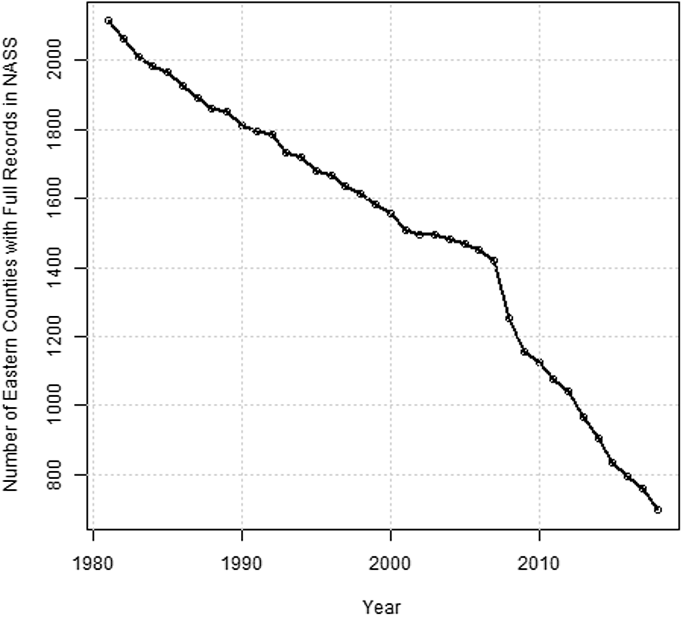
Figure 2. Number of counties east of the 100th Meridian line with a complete (balanced) panel of agricultural statistics records, 1981–2018.
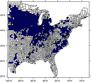
East of the 100th Meridian there were 2,471 counties in the 2012 Agricultural Census county boundary map. As shown in Figure 2, the number of observations available to construct a balanced panel with records for all years has declined sharply. To build a balanced county panel, this study uses 1,042 counties (1981–2012) that, together, were the largest of counties available for analysis to construct a balanced panel with a minimum of 1,000 observations. This is about 57% of the total number of counties with at least one reported year of corn growing history detailed in Appendix A2. The difficulty of acquiring balanced data likely explains why there has been scant literature using spatial econometrics to study crop yield response compared to Ricardian approaches. There would be a concern about selection bias from removing counties with unbalanced yield histories. We implement the robustness check for three benchmark models (Pooled, FE, and RE) before and after removing unbalanced yields for 1981–2012 (see Table S4 in Supplemental Materials). The results show that the selection bias in our analysis is not likely to be serious, and this finding is consistent with results from the similar robustness checks adopted in Schlenker and Roberts (Reference Schlenker and Roberts.2009). The counties included in this study are shown in Figure 3.

Figure 3. Study area: dark blue counties (n = 1,042) with balanced data used for estimation and in-sample prediction analysis.
The remaining years (2013–2018) of corn yield data available from NASS are used to assess out-of-sample prediction performance. There are 38,344 (33,344 for 1981–2012 and 5,622 for 2013–2018) total county corn yield observations in the study area (Figure 3) for the entire in-sample and out-of-sample period from 1981 to 2018. Among these, 5,622 (14.43%) observations are used for out-of-sample prediction. To summarize, we first use balanced panel data (total 33,344 observations) from the N = 1,042 counties for T = 32 years for the estimation and in-sample model fitting, and then we implement out-of-sample predictions using data from the same counties in 2013–2018. To further investigate prediction performance, we also implement year-stratified bootstrapping using the 1981–2012 data detailed in the next section.
The minimum and maximum temperature daily PRISM data for March to August 1981–2018 are used to calculate GDDs. Using the pre-processed daily weather data from Yun and Gramig (Reference Yun and Gramig.2019), we build −60 to +60°C heat exposure length in 1°C increment as Schlenker and Roberts (Reference Schlenker and Roberts.2009) did. Then, we sum the heat exposure lengths to get the GDDs between 8 and 32°C and above 34°C for Equations (3)–(10), and the −1–30°C bins specified in Equations (3’)–(10’). The total growing season precipitation is the sum of daily total precipitation in PRISM from March to August (1981–2018).
In this study, we carefully select soil variables for RE models. Much of the previous literature adopted soil structure (e.g., proportion of sand, clay, and silt) and other properties such as drainage or soil erosion factors as separate variables. For example, Schlenker et al. (Reference Schlenker, Hanemann and Fisher.2006) and Baylis et al. (Reference Baylis, Paulson and Piras.2011) used the percentage of clay and soil permeability. It is, however, important to note that soil structure is one of the major determinants of other soil characteristics that may more directly relate to crop yield or weather induce crop stress. Higher clay content means higher permeability, and more sandy soils have higher drainage class and erosion factors. Including soil texture and other related soil property variables in a regression together, therefore, may double-count soil characteristics. Wolkowski (Reference Wolkowski2005) classifies 10 important soil quality factors in crop production systems. Among those, we selected four quantifiable factors—organic matter, K factor, water holding capacity, and soil pH—to avoid the double-counting issue. Footnote 6 These variables are extracted from Yun and Gramig (Reference Yun and Gramig.2019) that provides the depth-weighted average soil factors across soil horizons from gSSURGO on land where agricultural production occurs. The summary statistics of variables used in prediction analysis are in Table 2.
Table 2. Summary statistics
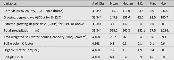
Notes: Weather variables calculate for March to August; Summary statistics of soil variables are calculated only for agricultural land in 1,042 counties based on four separate years of the National Land Cover Database spanning the study period from Yun and Gramig (Reference Yun and Gramig.2019).
In the regression, we take the log of crop yields as y it = log (corn yieldit + 1). We use Yun and Gramig’s (Reference Yun and Gramig.2019) agricultural land use and land cover adjusted soil characteristics based on the 1992, 2001, 2011, and 2016 US Geological Survey’s National Land Cover Database (NLCD), and we match them to the years in the balanced panel data (1992 to 1981–1995; 2001 to 1996–2003; 2011 to 2004–2013; and 2016 to 2014–2018). The soil variable summary statistics, therefore, are the descriptive statistics for soil underlying agricultural land uses in the 4 years of the NLCD.
Choosing a proper spatial weights matrix is one of the difficult questions in spatial econometrics. Figure 3 illustrates why a spatial weights matrix based on continuity cannot be applied because there are a few isolated counties that have no direct neighbors. In the recent Ricardian literature, Baylis et al. (Reference Baylis, Paulson and Piras.2011) adopted the 10-nearest neighbors, and Dall’erba and Dominguez (Reference Dall’erva and Dominguez.2016) used the neighbors within a 240 km cut-off distance. This study selects the six-nearest neighbors to construct the spatial weights matrix; as shown in the results, we believe this choice of the spatial weights works properly.
4. Estimation Results and Prediction Performances
We estimate 14 different model specifications. First, we estimate the response coefficients using the balanced panel data (1981–2012). The estimation results for the models in Equations (3)–(10) are presented in Table 3. The full estimation results are available from Table S2 in Supplemental Materials. Following Elhorst (Reference Elhorst2014) and conventional usage, we provide abbreviated model names in the first row of Table 3.
Table 3. Estimated spatial coefficients and in-sample prediction performances
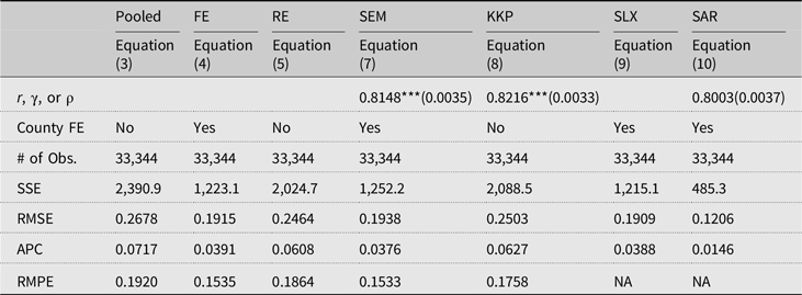
Notes: * p < 10%, ** p < 5%, and *** p < 1%; Standard errors are reported in parentheses; County FE, county fixed effects; SSE, sum of squared errors; RMSE, root mean squared errors; APC, Amemiya’s prediction criterion; RMPE, root mean squared prediction errors for 2013–2018 out-of-sample period. The full estimation results are available from Table S2 in the provided Supplemental Materials.
The estimation results in Table S2 show that most individual estimates are significant, and their signs are generally in the same direction. Compared to the FE model that excludes time-invariant variables relevant to yield determination, the soil variables in the RE model are statistically significant. As discussed in the specification section, this empirically supports the argument that location FE terms capture county-specific soil characteristics. In the SEM, KKP, and SAR spatial econometric models, all spatial response coefficients (r, γ, and ρ) are highly significant. One interpretation caveat is needed for the SLX model of Equation (9). The spatially lagged weather variables were applied to all weather variables following the general specification rules in spatial econometrics, including the squared terms. The primary issue here is how to interpret the meaning of squared terms. If all weather terms are linear, then the spatial dependence structure is apparent. The squared terms, however, do not clearly explain how the spatial dependence of the first-order terms is spatially connected to the squared terms.
We do not present the overall goodness-of-fit or relevant overall significance test statistic because the estimation methods are different across models. To compare in-sample prediction performance, we calculate the squared sum of errors, root mean squared errors, and Amemiya’s prediction criterion. Considering all three prediction performance metrics, the best in-sample prediction model is the SAR model (10). The second best is either the FE or SLX model. Since these models are frequently adopted to forecast future outcomes, we estimate the predicted log corn yields using the 2013–2018 data that are not used for the estimation. The root mean squared prediction errors (RMPE) in the last row of Table 3 is a metric of their prediction performance. The RMPE results indicate that the SEM model (7) performs slightly better than the FE model (4).
It is important to note that the SLX and SAR models are not compatible with this prediction analysis because the data set is an unbalanced panel. Notably, we do not have corn yield data or spatial weights (regions not included in the spatial weights matrix) for all neighbor counties. If we are interested in future prediction to investigate the impact of climate change, the SAR and SLX are unusable. The prior Ricardian literature examined the SAR specification estimating the direct and indirect marginal effects for future prediction. We do not estimate these effects because they are not directly comparable to other models in this study.
In Table 4, we repeat the same estimation and prediction analysis for models specified using nonlinear GDD bins in equations (3’)–(10’). The full estimation results are available from Table S3 in Supplemental Materials.
Table 4. Estimation results with nonlinear GDD bins
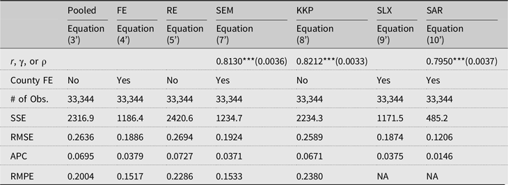
Notes: * p < 10%, ** p < 5%, and *** p < 1%; Standard errors are reported in parentheses; County FE, county fixed effects; SSE, sum of squared errors; RMSE, root mean squared errors; APC, Amemiya’s prediction criterion; RMPE, root mean squared prediction errors for 2013–2018 out-of-sample period. The full estimation results are available from Table S3 in the provided Supplemental Materials.
Like Table S2, most of the estimates are statistically significant, and signs of estimates are similar across models. Note that we put the constant (0th order) term of the eighth-order Chebyshev polynomials in the intercept, FE, or error terms. Since each coefficient of the Chebyshev polynomials does not mean the size of GDDs, the signs of the estimates cannot be interpreted directly. Similar to Equation (9) in Table 3, the estimates of the spatially lagged terms in SLX model (9’) do not have direct meaning either. The SAR model has the best in-sample prediction performance. Again, the RMPE is not applicable in the SAR and SLX models. In the out-of-sample RMPE, the FE model performs slightly better than the SEM.
Across Tables 3 and 4 (in addition to Tables S2 and S3), it is important to note that the two RE models (RE and KKP) perform relatively poorly compared to the other models. The in-sample prediction capability of these models is also weaker after adopting the eighth-order polynomial in GDDs. The FE and SEM models, however, perform better in both in- and out-of-sample prediction with the nonlinear polynomial GDDs. Given that the nonlinear temperature effects were empirically proven in the previous literature, we believe that the RE models are not a good predictor in these data.
To extensively scrutinize prediction performance, we implement an additional out-of-sample approach with the year-stratified bootstrap following Schlenker and Roberts (Reference Schlenker and Roberts.2009). Due to the considerable correlation across counties, this year-to-year sampling is able to preserve the location-specific correlations within a year and reflect annual random weather fluctuations. We first randomly selected 32 individual years of data with replacement from the entire 32-year panel (1981–2012). The first 27 years of randomly drawn data are used for the estimation, and the remaining 5 years (15.6% of the whole data) are used to evaluate out-of-sample prediction. We replicate this process 1,000 times and got the RMPEs as a distribution for the 14 competing models. The results are summarized in Table 5.
Table 5. Model comparison for prediction accuracy
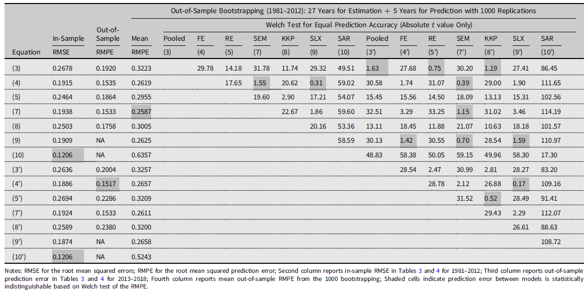
The second and third columns are the in-sample and out-of-sample prediction performance statistics described in Tables 3 and 4. The fourth column is the mean of the RMPE from 1,000 bootstrap replications. The gray-colored cells indicate the best-performing model for each prediction performance metric. The remaining 14 columns report a pairwise Welch t-test against the null hypothesis of equal mean RMPE given unequal variances. Failure to reject the null hypothesis indicates that two models provide the same level of prediction accuracy. The figures in the cells are the t statistics. Since the sign of t statistic does not deliver any meaningful information, we omit the signs for simplicity. Because of the symmetry, we also present the upper diagonal cells only. The gray-colored cells indicate the cases that we cannot reject the null at any significance level.
The most directly noticeable results in Table 5 is that the SAR model of Equation (10’) produced the most inaccurate prediction performances. The mean RMPEs for both Equations (10) and (10’) are the largest two among all 14 specifications. In addition, the Welch tests showed that both are the two most different values from all others. In the prior Ricardian approaches, Baylis et al. (Reference Baylis, Paulson and Piras.2011) and Dall’erba and Dominguez (Reference Dall’erva and Dominguez.2016) empirically demonstrated that the SAR model worked well to explain land values. Our results, however, show that the SAR model is not likely to be a proper predictor in the crop yield response function.
The best three out-of-sample prediction performances are Equations (7), (7’), and (4), that is, the lowest three mean RMPE in the fourth column. The Welch test results provide evidence that these three models perform in a statistically identical manner for out-of-sample prediction (see the SEM model (7’) in Table 5). Interestingly, all three are FE models. The first two are the SEM specification. Considering that Equation (4’) from Schlenker and Roberts (Reference Schlenker and Roberts.2009) is the most popular specification in the literature, this result empirically suggests that the inclusion of spatial correlation in the error terms of crop yield response functions will enhance prediction capability in econometric models of crop yield response.
5. Conclusion and Discussion
Due to the enhanced accessibility and ability to manage weather, climate, and soil data, climate econometrics (Hsiang, Reference Hsiang2016) has become one of the most widely used tools to forecast the impact of climate change on agriculture. In the literature, the Ricardian approach and crop yield response function estimation are the two most popular approaches to climate econometrics. This study provides a counterpart study to previous Ricardian analyses by accounting for spatial correlations using spatial econometric models of crop yield response functions. To this end, this study first demonstrates the possible conceptual explanations and empirical applications of modeling spatial correlation in econometrics to specify 14 competing models. Using county-level corn yield response to weather and time-invariant location characteristics in panel regressions, we perform in-sample, out-of-sample, and bootstrapping out-of-sample predictions. Based on these prediction performance comparisons, four major implications emerge.
First, spatial aggregation bias could be a significant source of spatial correlation between error terms in empirical specifications of crop yield response functions. This study carefully discussed the possible spatial correlation in common functional forms and models and compared the prediction performance in various ways. The models with spatially dependent error structures—the SEM specification of FE models in Equation (7) and (7’)—demonstrated generally powerful prediction performance among 14 competing models studied. In spatial econometrics, omitted variable bias has been emphasized as a motivation to use the SEM model (LeSage and Pace, Reference LeSage and Pace.2009). Using three propositions and empirical examples, we discuss how spatial aggregation of weather variables can generate spatial correlation in the error terms of econometric models of crop yield response functions as well. Fezzi and Bateman (Reference Fezzi and Bateman.2015) also found that spatial aggregation could lead to estimation bias by comparing the estimates of Ricardian models using field and county data. It is worth noting that nonspatial FE in Equation (2) and (2’) exhibit almost equivalent prediction capability to SEM with FE. Because the estimated spatial weights matrix parameter is statistically significant and strongly positive (about 0.8), however, the SEM specification of the FE model that controls for spatial correlations in the error terms is expected to achieve more accurate statistical inference compared to FE. The relatively better prediction performance and statistical inference benefits of the SEM model in this study, therefore, theoretically and empirically supports the use of FE model specifications with nonparametric error structures used in Schlenker and Roberts (Reference Schlenker and Roberts.2009) and the SEM model specification in Schlenker et al. (Reference Schlenker, Hanemann and Fisher.2006).
Second, the spatial lag specification known as SAR should be used cautiously for prediction performance. Despite the SAR specification being one of the most popular models used in spatial econometrics, our Welch test for out-of-sample prediction accuracy demonstrated that the RMPEs of Equations (10) and (10’) deviate seriously from the best-performing prediction models. This result illustrates that the SAR specification may perform poorly when used for prediction. As mentioned earlier, a crop yield response function is generally used as a base model to predict weather or climate impacts on crop yields. The SAR-based predicted responses may overemphasize the impact of climate change on crop yields compared to an unknown counterfactual. The SAR specification is not applicable for prediction of future crop yields because neighbors’ future yields are unknown, potentially resulting in misleading the direct and indirect marginal effects. The SAR model, however, outperforms all other models when it comes to in-sample prediction. This best performance suggests the possibility of using SAR as a predictor of missing contemporaneous crop yields described in Johansson et al. (Reference Johansson, Effland and Coble.2017). In this setting, the SAR specification would need to prove its empirical prediction capability compared to alternatives like the Bayesian kriging in Park et al. (Reference Park, Brorsen and Harri.2019).
Third, we argued that the counterpart of the FE model of crop yield response is the RE model with time-invariant soil variables. The FE term in a crop yield response function controls for location-specific soil characteristics and all other variables that are generally assumed to be time-invariant. If the RE specification is motivated by a suspected omitted weather variable, the soil characteristics should stay in the RE model argued in Equation (5). It is well known, however, that soil attributes like organic matter are dynamic and may vary across time based on management and cropping history. If the dynamic soil variables were available to researcher, then the FE model should include soils in addition to the FE terms as a counterpart to RE. Unfortunately, because those soil variables are unavailable in general, we cannot use the standard statistical test to choose between the FE and RE models such as the Hausman test or spatial Hausman test between Equation (4) and (5).
Lastly, the selection of prediction models requires careful performance comparisons. Our results demonstrate that the FE or SEM with FE better predicts crop yield response among 14 competing models based on three different prediction performance metrics. Even though this study considered the most common specifications of crop yield response functions, an extensive set of spatial panel specifications are also available. Elhorst (Reference Elhorst2014) suggested the use of model specification trees starting from the general nesting spatial model, including the spatial Durbin specification. It is of course possible that an empirical specification test could end up selecting alternative models (not FE or SEM with FE). Also, we can consider more flexible model specifications through variable transformations, for example, inverse hyperbolic sine transformation. Footnote 7 In reality, it is difficult to consider all combinations of model specifications and possible selection criteria, and given so many possible options, it may be hard to know where to start for a given application. This study provides an example of specification and selection strategies, emphasizing the necessity of prediction performance comparisons with extensive competing models to reduce the bias from model specification and selection criterion.
Despite our efforts on specification and performance analysis, we acknowledge that there are at least three issues we have not addressed that require additional study. First, our study focuses on finding the best predictive model rather than the most precise parameter estimates. Having good estimates is essential for causal inference, but identification strategies or their implications are beyond the scope of the current study. Second, well-balanced yield data are required to apply spatial econometric estimation methods, and spatial econometric models for unbalanced panel data are needed. Because of the lack of balanced data that conforms to the requirements of existing estimation methods, it is not surprising that spatial econometric analysis of crop yield response remains uncommon despite spatial Ricardian models having appeared regularly in the literature for some time. Lastly, more extensive research is necessary to generalize the findings in this study. Our results are valid for the given data that are commonly available for crop yields. To go beyond the practical implications here, to provide general implications, crop yield response functions need to be studied over various spatial units, regions, and performance criteria.
Supplementary Material
For supplementary material for this article, please visit https://doi.org/10.1017/aae.2021.29
Author Contributions
Conceptualization, S.D.Y. and B.M.G.; Methodology, S.D.Y. and B.M.G.; Formal Analysis, S.D.Y.; Data Curation, S.D.Y.; Writing Original Draft, S.D.Y. and B.M.G.; Writing-Review and Editing, S.D.Y. and B.M.G.; Supervision, S.D.Y. and B.M.G.; Funding Acquisition, B.M.G.
Financial Support
Authors are grateful for financial support through the “Useful to Usable (U2U): Transforming Climate Variability and Change Information for Cereal Crop Producers” project provided by United States Department of Agriculture (USDA) National Institute for Food and Agriculture (NIFA) competitive award no. 2011-68002-30220. Yun and Gramig also received support from USDA-NIFA Hatch multi-state project W-4133 “Costs and Benefits of Natural Resources on Public and Private Lands.” The findings and conclusions in this article are those of the authors and should not be construed to represent any official USDA or U.S. Government determination or policy.
Competing Interests
Authors disclose that there are no relevant financial or nonfinancial competing interests to report.
Data Availability Statement
The original data used in this manuscript are publicly available through the corresponding author’s GitHub repository: https://github.com/ysd2004/spatialcropyieldJAAE. All underlying data processed to create model variables come from peer-reviewed and publicly accessible sources.
Appendix
A1. Specification of nonlinear heat exposure in Equations (3’)–(10’)
Schlenker and Roberts (Reference Schlenker and Roberts.2009) adopted three different specifications on the heat integrals: step function, mth order Chebycheb polynomials, and piecewise linear. Because of the smoothness in heat exposure, we use the Chebyshev polynomial approximation. The mth order Chebyshev polynomial representation of $\int _{\underline{h}}^{\overline{h}}g(h)\varphi _{it}dh$
is:
$\int _{\underline{h}}^{\overline{h}}g(h)\varphi _{it}dh$
is:
 $$\mathop \smallint \limits_{\underline h }^{\overline h } g(h){\phi _{it}}dh = \mathop \sum \limits_{k = 1}^m {\omega _k}\mathop \sum \limits_{i = - 1}^{30} {T_k}(h + 0.5)[{_{it}}(h + 1) - {_{it}}(h)] = \mathop \sum \limits_{k = 1}^m {\omega _k}{x_{it,k}}$$
where T k (⋅) is an mth order Chebyshev polynomial node and ω k is its coefficient. Because Schlenker and Roberts (Reference Schlenker and Roberts.2009) proved the eighth-order polynomial worked the best, this study also adopts the eighth-order specification.
A2. Corn yield data
East of the 100th Meridian line, there were 2,471 counties covered by the 2012 Agricultural Census. Figure A1 is the histogram of corn yield frequencies for 1981–2012. The number of county-years that corn was grown in at least 1 year was 58,468 for 1981–2012 is given by the sum of all frequencies in Figure A1. Among them, 1,042 counties have records for all 32 years. The proportion of county-years used in the estimation, therefore, is 57% (1,042 counties × 32 years / 58,468).
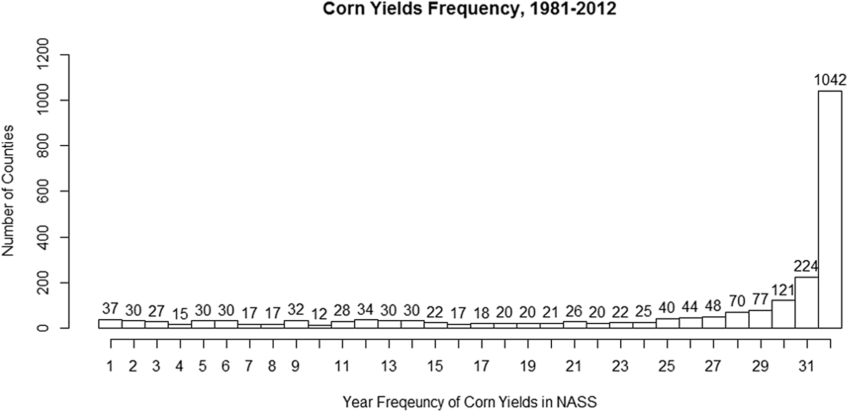
Figure A1. Histogram of corn yield frequencies by number of total counties reported by USDA-NASS, 1981–2012.


 Open access