


1. Introduction
Risk is inherent to agriculture and can broadly be classified into business risk and financial risk, where the former arises from production and price risk and the latter from the proportion of capital raised from other business sources (Hardaker et al., Reference Hardaker, Lien, Anderson and Huirne2015; Komarek, De Pinto, and Smith, Reference Komarek, De Pinto and Smith2020). According to reports published by the Organisation for Economic Co-operation and Development (OECD), farm enterprises in Australia face high production and price risks (Kimura, Antón, and Lethi, Reference Kimura, Antón and Lethi2010; Kimura and Antón, Reference Kimura and Antón2011). To make informed decisions, farmers must be able to assess their financial viability and potential business risks.
Australia’s dairy industry was the country’s third largest rural industry with a farmgate value of A$4.3 billion in the financial year 2017–2018. Australia’s 5,699 dairy farms produce a total of 9.3 billion liters of milk annually (Dairy Australia, 2018). The state of Victoria alone hosts 3,520 dairy farms, which produced 5.57 billion liters of milk in 2018–2019 (Agriculture Victoria and Dairy Australia, 2018), or approximately 67% of national milk production (Dairy Australia, 2020a). However, dairy farmers are facing a continuous cost price squeeze amid a challenging global environment that suppresses milk prices and raises feed costs with drier and hotter weather conditions (Dairy Australia, 2019; Mallawaarachchi et al., Reference Mallawaarachchi, Nauges, Sanders and Quiggin2017).
While it is impossible to know what will happen in the future, simulations allow one to create risk profiles by generating a large number of scenarios, including extreme cases, offering a way to study the effects of factors such as weather and price variations. Thus, results from simulation studies can approach questions such as “What is the chance of making a profit in ten years?” given known variabilities. In other words, our simulations allow stakeholders to assess risks and financial viability in a probabilistic way, which in turn aids informed decision-making (Albright and Winston, Reference Albright and Winston2019; Lehman and Groenendaal, Reference Lehman and Groenendaal2020).
Among the earlier simulation-based Australian dairy industry risk studies, Sinnett, Ho, and Malcolm (Reference Sinnett, Ho and Malcolm2017) analyzed a case study dairy farm in northern Victoria to highlight the need to assess financial risk before deciding on expanding the business. Ho, Malcolm, and Doyle (Reference Ho, Malcolm and Doyle2015) tested the impact of changing water availability on two dairy farms in northern Victoria and the associated profit risk. That study concluded that in order to maintain profit, case study farms needed to make changes to their farming systems such as additional supplementary feeding and/or using a partial mixed ration system. Henty et al. (Reference Henty, Ho, Auldist, Wales and Malcolm2020) analyzed the impact that changing the feeding regime on a farm in south-west Victoria had on profit. The system of grazed pasture, with grain-fed in the dairy and forage fed in the paddock, was changed to a partial mixed ration (PMR) or a formulated grain mix (FGM) feeding system, with the later found to be more profitable. All three of the above studies used Palisade’s @RISK for the analysis.
Browne et al. (Reference Browne, Kingwell, Behrendt and Eckard2013) compared 14 representative farm enterprises in south-eastern Australia under low, average, and high rainfall scenarios. The production systems included Merino fine wool, prime lamb, beef cattle, milk, wheat, and canola. The researchers concluded that profitability of these enterprises had been affected more by changes in rainfall than by commodity prices. Dairy enterprises were the most profitable on a dollars per hectare basis than the other farming options.
With the exception of Browne et al. (Reference Browne, Kingwell, Behrendt and Eckard2013), the above studies simulated the input variables from their individual univariate distributions without considering the dependencies between the input variables. However, when a dairy farm is considered, variables that impact the profitability are likely to be dependent on each other. For example, when herd cost increases, shed cost and cash overhead costs are likely to increase as well. As these variables naturally move together, it is important to estimate and include the dependency structure between the variables in any simulation study. To this end, copula-based models, which will be adopted in this work, are flexible tools for revealing multivariate distributions that capture the statistical relationships, such as non-linear dependence, among the input variables (Manner and Reznikova, Reference Manner and Reznikova2012), while allowing the univariate distributions to be estimated separately (Zhu, Ghosh, and Goodwin, Reference Zhu, Ghosh and Goodwin2008). While Browne et al. (Reference Browne, Kingwell, Behrendt and Eckard2013) included the rank correlations between the variables in their simulations, the method of copula was not used.
Originating in financial studies, copula-based methods have recently been adopted in agricultural studies. For example, Ribeiro et al. (Reference Ribeiro, Russo, Gouveia and Páscoa2019) and Vergni, Todisco, and Mannocchi (Reference Vergni, Todisco and Mannocchi2015) studied the risk of drought using copulae on various crops. Copula-based approaches have also been widely used in the area of crop insurance. To list a few, Ahmed and Serra (Reference Ahmed and Serra2015) studied revenue crop insurance for orange and apple sectors; Marin et al. (Reference Marin, John, Cameron and Brian2014) studied livestock gross margin insurance for dairy cattle (LGM-Dairy) premiums; Goodwin and Hungerford (Reference Goodwin and Hungerford2015) evaluated the impacts of multiple sources of risk on crop insurance premiums, while Ramsey, Ghosh, and Goodwin (Reference Ramsey, Ghosh and Goodwin2020) studied the flexibility of various type of copulae in modeling novel price coverages in crop revenue insurance.
Despite the versatility of the copula-based methods, to the best knowledge of the authors, these have not been applied to studying the risk profiles of dairy farms, under whole-farm scenarios, in the Australian context. The present research applies the method of copula to compare regions in the nation’s highest milk-producing state of Victoria, assessing farm stability and profitability. Specifically, we simulate the risk profiles for representative farms in each of the three dairy regions: North (N), Gippsland (G), and South West (SW), and compare their business and financial risks. The Gippsland and South West dairies are in the higher rainfall parts of Victoria (Figure 1), south of the Murray Darling Basin (MDB), while the Northern dairy region is within the MDB, which has suffered water and feed shortages.
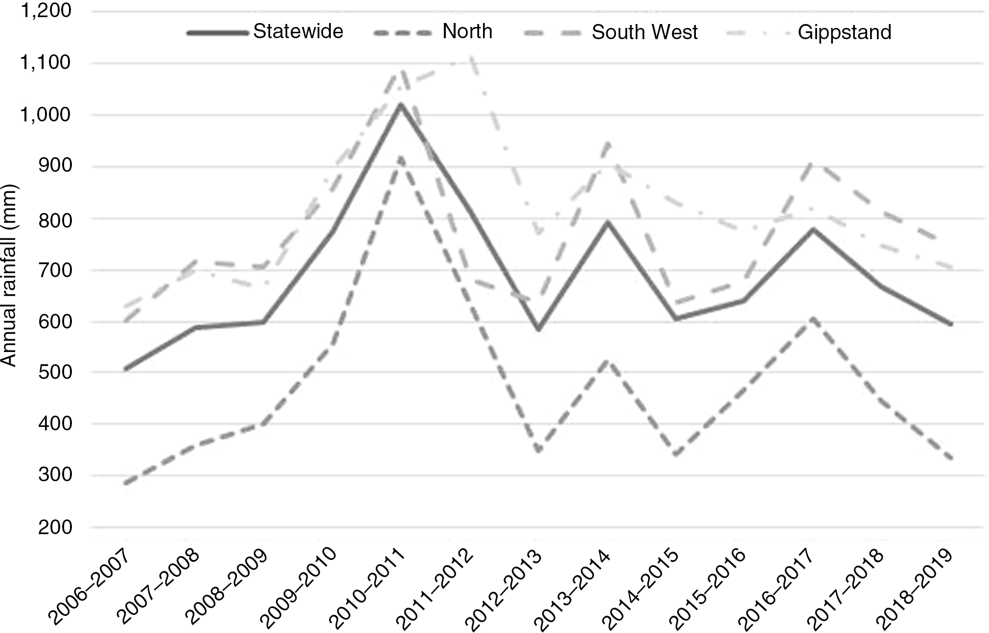
Figure 1. Annual rainfall (mm) in the Victorian state and its North (N), Gippsland (G), and South West (SW) regions from July 2006 to June 2019. Source: Agriculture Victoria and Dairy Australia (2019) and the earlier published reports.
In 2012, Australia’s largest processor of dairy products, Murray Goulburn, announced it would be stopping powdered milk production at its factory at Rochester, northern Victoria, with the loss of 64 jobs. This was due to lower milk production in northern Victoria and the southern Riverina regions. Cheese and whey processing would continue on the site, however (Price, Reference Price2012). In northern Victoria, total water available for irrigation has been reduced due to the Murray Darling Basin Plan and a period of below average inflows to the major storages. Participating in the water market is now just part of doing business for most dairy farms in the Murray Dairy Region (Dairy Australia, 2015). Dairies in Northern Victoria have faced challenges of drought with higher cost irrigation water and feed. Water entitlements were surrendered by dairies in government buy-back programs to support environmental goals. The Victorian Environmental Water Holder (2020), a statutory body, trades water to improve the health of Victoria’s rivers and wetlands.
In 2018–2019, the average dairy farm purchased 41% of the water they used on the temporary market, while temporary water purchases by horticultural farm’s were only 39% of their use that year, a significant increase on previous years (Australian Competition and Consumer Commission, 2021, p. 113). Another estimate is that “approximately 60% of water used by dairy is sourced from the temporary trade market annually” (Dairy Australia, 2020b).
Due to the heterogeneity in conditions, farms in different regions are subject to different probability distributions of the variables underlying the copulae. Therefore, a different risk profile was estimated for each region. This study’s risk profiles were constructed using simulation methods based on the copula modeling functions available in @RISK 8.2 (Palisade Corporation, 2021). A whole-farm approach was taken to integrate the three financial statements, that is, balance sheets, profit and loss budgets, and cash flows to capture wealth generation, efficiency, and liquidity of the representative farms, which are pivotal to the success of any business.
2. Methods
Business and financial risks for three representative farms, one in each of the three dairy regions, were analyzed. Figure 2 illustrates the locations of the three regions. The economic, financial, and biophysical aspects of the three representative farms were based on thirteen years of historical time series data from 2006–2007 to 2018–2019, published by Agriculture Victoria and Dairy Australia (2019) which reported averages based on 25 farms, whose identities are protected, in each region.
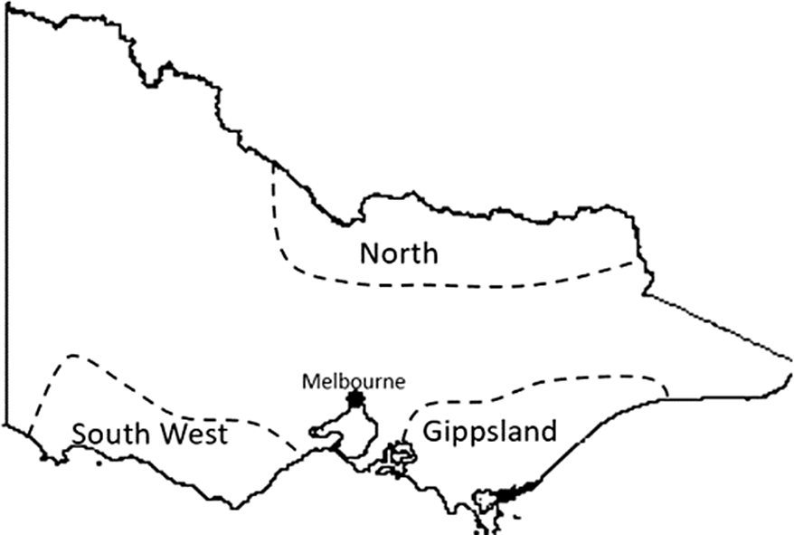
Figure 2. Map of Victoria, Australia, showing the approximate locations of the farms in the three dairy regions: North (N), Gippsland (G), and South West (SW) based on documentation by Agriculture Victoria and Dairy Australia (2019).
Our analysis was carried out in two steps. In the first step, key performance indicators (KPIs) were defined based on the simulated financial statements using well-established farm financial management and economic approaches (Barry and Ellinger, Reference Barry and Ellinger2012; Kay, Edwards, and Duffy, Reference Kay, Edwards and Duffy2016; Malcolm, Makeham, and Wright, Reference Malcolm, Makeham and Wright2005; Nuthall, Reference Nuthall2011). The data used for this analysis assigned all prices and costs over time in “real” dollar values based on 2018–2019 dollar equivalents by the consumer price index (CPI) to adjust for inflation. In the second step, joint multivariate distributions of historical production, price, and cost data were estimated through copula functions, which account for the dependency among these variables over the historical period (2006–2007 to 2018–2019). Randomly drawn decadal samples from multivariate simulations were used to calculate budget details and decadal cash margins from which KPIs were summarized for each setting in 10,000 simulated iterations.
An opening balance sheet (Table 1) captured the net worth of opening values for 2018–2019 of three farms. The future growth/decline of business wealth was then based on risk captured in financial statements for each year of a 10-year (decadal) iteration. The risk profiles described as cumulative distribution functions (CDFs) of decadal ending net cash balances were generated to represent the probabilistic nature of risk in growth or decline of equity. The following KPIs were used in our analysis, where details can be found in Godfrey et al. (Reference Godfrey, Nordblom, Ip, Robertson, Hutchings and Behrendt2021): debt to assets (D:A or solvency ratio), changing debt to equity (D:E or gearing ratio), return on capital (ROC) and return on equity (ROE), and net profit (NP) obtained from the financial statements for the decadal analysis. Cash flows were used to determine the net present value (NPV) with a real 4% discount rate and modified internal rate of return (MIRR) converting a nominal 6.5% interest rate as indicated by the Australian Bankers’ Association (2016). To compute MIRR, the capital was borrowed at 4%, and the rate at which the funds could be reinvested was 2%. Each representative farm’s liability was assumed to be debt financed by a bank overdraft facility at a real interest rate of 4% to meet payment obligations. In years when net farm income was negative, debt accumulated and compounded over time, whereas positive net farm income contributed to the retirement of debt. The positive cash balance was used to offset the interest payments. Farmland was assumed to be appreciating at 3.3% per annum in real terms (Rabobank, 2020) while the value of plant and equipment depreciated at 5% per annum using the declining balance method. The data on inflation to calculate the real rate of returns were obtained from the ABARES (2020).
Table 1. Financial statements for regional means (n=25) of three Victorian dairy regions: North (N), Gippsland (G) and South West (SW). The table shows opening balance sheets and equity for each representative farm and the profit and loss (P&L) budget model to calculate probabilistic earnings before interest and tax (EBIT) and net farm profits (NP) based on the method used by Agriculture Victoria and Dairy Australia (2019). Table also shows the cash flow estimation method
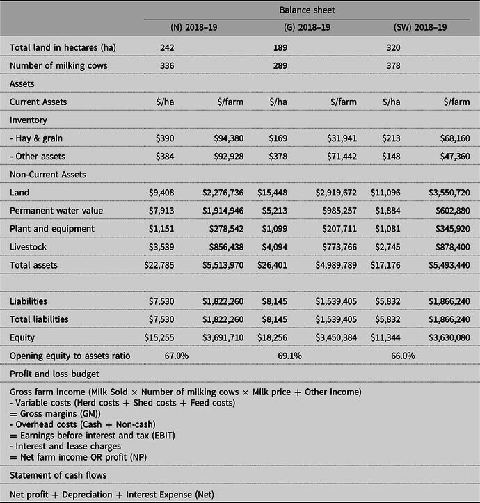
Source: Agriculture Victoria and Dairy Australia (2019). Opening balance sheet average estimates for N, G, and SW Victorian dairy regions have been taken from Table B8 on p. 78, Table C8 on p. 86 and Table D8 on p. 94. Profit and loss budget 13 years historical data taken from Table B9 on p. 79, Table C9 on p. 87 and Table D9 on p. 95. Other income for all 13 years was calculated as a percentage of total gross income. The annual average depreciation percentage for each year as a non-cash overhead cost was taken from the previous reports. The livestock trading account, that is, cost of replacements for each year of analysis, are based on the Agriculture Victoria and Dairy Australia (2019) and past thirteen years of reports.
In each simulated year from 1 to year 10, net farm income was calculated based on simulated prices (P), quantities (Q) and costs. Each variable was a random variable, and all were governed by a joint distribution. In this sense, the net farm income can be considered as a non-linear combination of all the variables involved. The multivariate distribution of all variables had to be estimated from historical data in order to simulate the net farm income. To this end, the method of copula was used as detailed in the procedures below.
First, individual univariate distributions were chosen and estimated using the maximum likelihood method in @RISK8.2 (Palisade Corporation, 2021), with the option “Bounded, But Unknown” selected for both the “Lower Limit” and “Upper Limit”, to avoid illogical bounds being fitted. The best-fitted distributions were selected based on the Akaike information criterion (AIC) and were visually checked based on the histograms overlayed with the fitted density curves. Second, these univariate distributions were combined through a copula function. The method of copula is based on Sklar’s theorem (Reference Sklar1959), which states that the joint distribution of two variables can be represented as a function called copula of individual univariate distributions. Mathematically speaking, we have
 $${F_{XY}}\left( {x,y} \right) = {C_\theta }\left( {{F_X}\left( x \right),{F_Y}\left( y \right)} \right)$$
where
 ${F_{XY}}$
is the joint distribution,
${F_{XY}}$
is the joint distribution,
 ${F_X}$
and
${F_X}$
and
 ${F_Y}$
are the individual univariate cumulative distribution functions of
${F_Y}$
are the individual univariate cumulative distribution functions of
 $X$
and
$X$
and
 $Y$
, respectively, and
$Y$
, respectively, and
 $\theta $
represents the parameter(s). Equation (1) can also be expressed as
$\theta $
represents the parameter(s). Equation (1) can also be expressed as
 $${C_{uv}}\left( {u,v} \right) = {F_{XY}}\left( {F_X^{ - 1}\left( u \right),F_Y^{ - 1}\left( v \right)} \right),$$
where
 ${F^{ - 1}}$
denotes the inverse of the cumulative distribution function
${F^{ - 1}}$
denotes the inverse of the cumulative distribution function
 $F$
. While most copula functions are bivariate, higher dimensional copulae are becoming more popular (Shemyakin and Kniazev, Reference Shemyakin and Kniazev2017). Commonly used high-dimensional copulae include elliptical copulae such as multivariate Gaussian or
$F$
. While most copula functions are bivariate, higher dimensional copulae are becoming more popular (Shemyakin and Kniazev, Reference Shemyakin and Kniazev2017). Commonly used high-dimensional copulae include elliptical copulae such as multivariate Gaussian or
 $t$
and Archimedean copulae (Nelsen, Reference Nelsen2006) such as Clayton, Frank, and Gumbel (Aas et al., Reference Aas, Czado, Frigessi and Bakken2009). For example, for a random vector
$t$
and Archimedean copulae (Nelsen, Reference Nelsen2006) such as Clayton, Frank, and Gumbel (Aas et al., Reference Aas, Czado, Frigessi and Bakken2009). For example, for a random vector
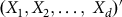 $\left( {{X_1},{X_2}, \ldots ,\;{X_d}} \right)'$
, the multivariate Gaussian copula admits the form
$\left( {{X_1},{X_2}, \ldots ,\;{X_d}} \right)'$
, the multivariate Gaussian copula admits the form
 $${F_{{X_1},\;{X_2}, \ldots ,\;{X_d}}}\left( {{x_1},{x_2}, \ldots ,{x_d}} \right) = {{\rm{\Phi }}_{d,R}}\left( {{F_{{X_1}}}\left( {{x_1}} \right),{F_{{X_2}}}\left( {{x_2}} \right), \ldots ,{F_{{X_d}}}\left( {{x_d}} \right)} \right),$$
where
 ${{\rm{\Phi }}_{d,R}}$
represents the
${{\rm{\Phi }}_{d,R}}$
represents the
 $d$
-dimensional mean-zero normal distribution with correlation matrix
$d$
-dimensional mean-zero normal distribution with correlation matrix
 $R$
. More examples can be found in Shemyakin and Kniazev (Reference Shemyakin and Kniazev2017). While both Gaussian and
$R$
. More examples can be found in Shemyakin and Kniazev (Reference Shemyakin and Kniazev2017). While both Gaussian and
 $t$
copulae belong to the class of elliptical copulae, the tail dependencies behave differently. In particular,
$t$
copulae belong to the class of elliptical copulae, the tail dependencies behave differently. In particular,
 $t$
copula possesses positive tail dependence while Gaussian copula has no tail dependence (Demarta and McNeil, Reference Demarta and McNeil2005). The copula function was estimated using the maximum likelihood estimation method in @RISK8.2 (Palisade Corporation, 2021). Various goodness-of-fit measures including AIC, Bayesian Information Criterion (BIC), and average log-likelihood values were considered in choosing the final copula type.
$t$
copula possesses positive tail dependence while Gaussian copula has no tail dependence (Demarta and McNeil, Reference Demarta and McNeil2005). The copula function was estimated using the maximum likelihood estimation method in @RISK8.2 (Palisade Corporation, 2021). Various goodness-of-fit measures including AIC, Bayesian Information Criterion (BIC), and average log-likelihood values were considered in choosing the final copula type.
These input distributions were then used to generate decadal (10-year) samples for probabilistic output distributions of profit and loss budgets and cash flows by performing 10,000 iterations of Monte Carlo simulation.
In our application, eleven input variables including price, quantity, and variable costs were considered. A full list of these variables can be found in Appendix A. Denoted by
 ${X_1},{X_2}, \ldots ,\;{X_{11}}$
the eleven variables. The whole procedure can be summarized as follows:
${X_1},{X_2}, \ldots ,\;{X_{11}}$
the eleven variables. The whole procedure can be summarized as follows:
-
1. For each variable
 $i$
, a univariate distribution
${F_{{X_i}}}\left( {{x_i}} \right)$
was fitted.
$i$
, a univariate distribution
${F_{{X_i}}}\left( {{x_i}} \right)$
was fitted. -
2. A copula function
$C$
which combines
${F_{{X_1}}}\left( {{x_1}} \right),\;{F_{{X_2}}}\left( {{x_2}} \right),\; \ldots ,\;{F_{{X_{11}}}}\left( {{x_{11}}} \right)$
was fitted. -
3. Based on the fitted copula
$C$
, an eleven-variate vector
$\left( {{u_1},\;{u_2}, \ldots ,\;{u_{11}}} \right)'$
was simulated where each
${u_i}$
is between 0 and 1. -
4. Through probability integral transform (Salvadori et al., Reference Salvadori, Michele, Kottegoda and Rosso2007), each
${u_i}$
was transformed back to its original scale through
${x_i} = F_{{X_i}}^{ - 1}\left( {{u_i}} \right)$
. -
5. Revenue and costs, and thus profit and loss, were then determined based on the simulated
${x_1},\;{x_2}, \ldots ,\;{x_{11}}$
. From year 1 onwards, the annual closing balances and various indices were then calculated. -
6. Steps 3–5 were repeated 10,000 times through Monte Carlo simulations. Risk profiles were created based on the empirical cumulative distributions of these simulated values.
-
7. The above steps were done for each of the three regions considered.


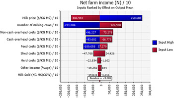
The impacts of input variables on the output variables were studied using sensitivity analysis, with an aim of determining the most influential factors affecting the financial outcomes of farms (Pianosi et al., Reference Pianosi, Beven, Freer, Hall, Rougier, Stephenson and Wagener2016). In @Risk, the simulated values of an input variable are first sorted in ascending order. These ordered values are then divided into ten equal bins. In our case, each bin would contain 1,000 values. The means of the output values in the “lowest bin” and the “highest bin” are computed and are reported in the form of a tornado graph, allowing one to tell which inputs have the most positive or negative impacts on the output variable.
3. Results
3.1 Fitted Distributions
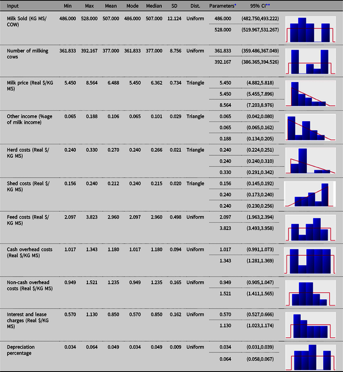
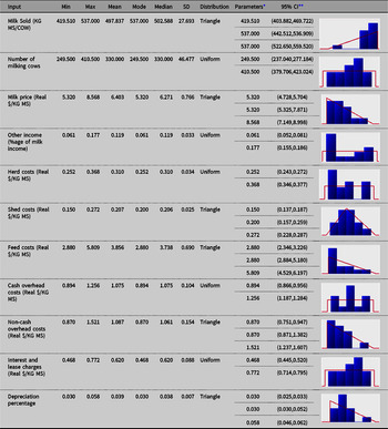
The fitted univariate distributions for the input variables (and the corresponding theoretical summary statistics) for each of the three regions are reported in Appendix A. Uniform, triangle and Pert distributions were found to provide the best fits to the data, according to AIC.
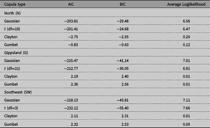
For the multivariate distributions, Gaussian copulae were fitted for the North and Gippsland regions, whereas the t copula was fitted for the South West region. Figures 3–5 illustrate the three regions, respectively, in terms of their rank correlation matrices used as parameters in fitting the copulae as well as scatter plot matrices based on the simulated data. Table 2 shows various goodness-of-fit measures for different types of copula for the three regions. Both elliptical copula types provided similar measures while Archimedean copulae were found to be less plausible. Since Gaussian and t copulae were found to be better, it does not seem to be much evidence of asymmetric dependence among the variables.
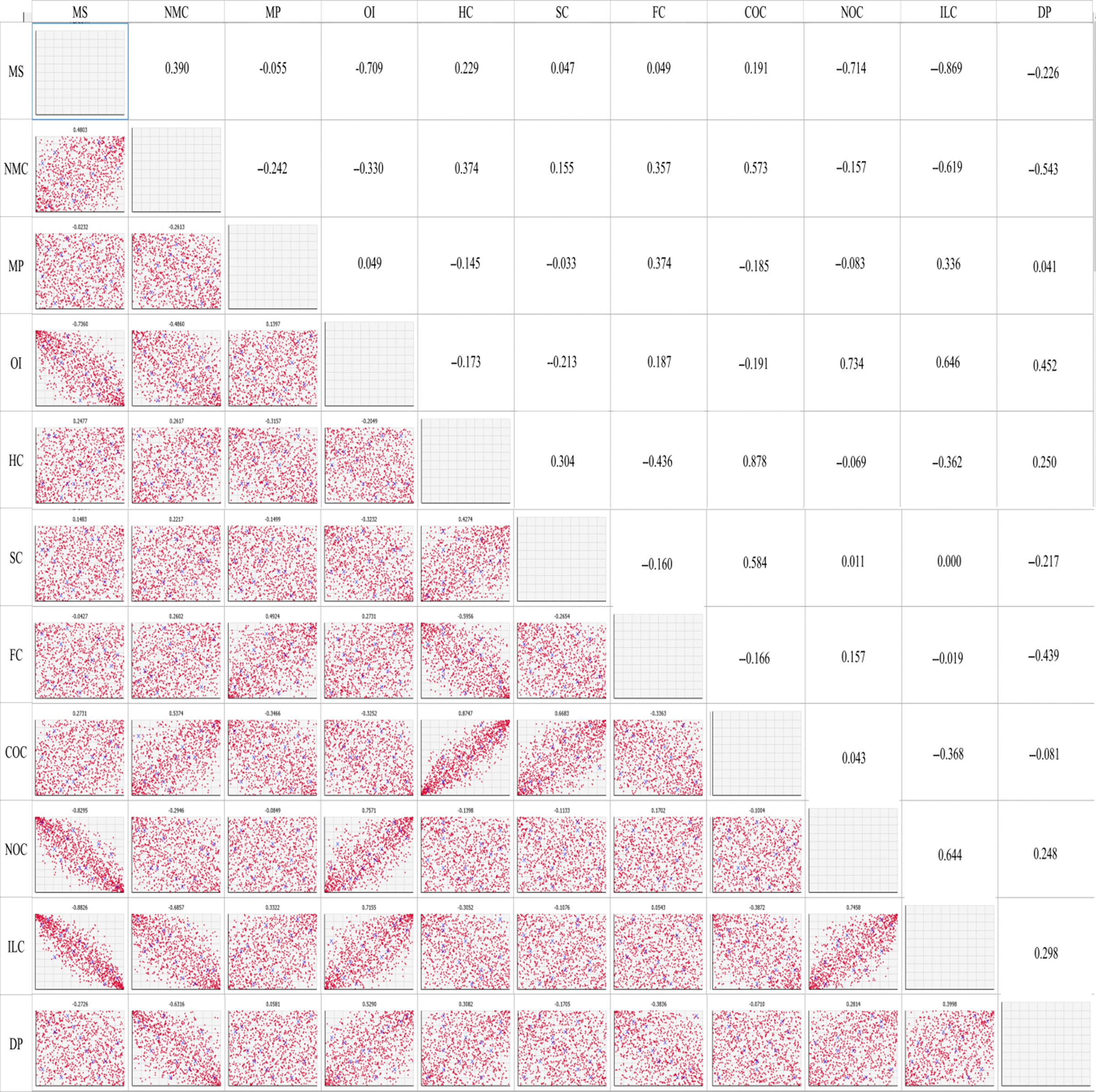
Figure 3. Copula-generated scatter plots (lower triangular cells) and estimated rank correlation matrix (upper triangular cells) used as parameters in the Gaussian copula for the North (N) Dairy Region. MS: milk sold, NMC: number of milking cows, MP: milk price, OI: other income, HC: herd costs, SC: shed costs, FC: feed costs, COC: cash overhead costs, NOC: non-cash overhead costs, ILC: interests and lease charges, DP: depreciation percentage.
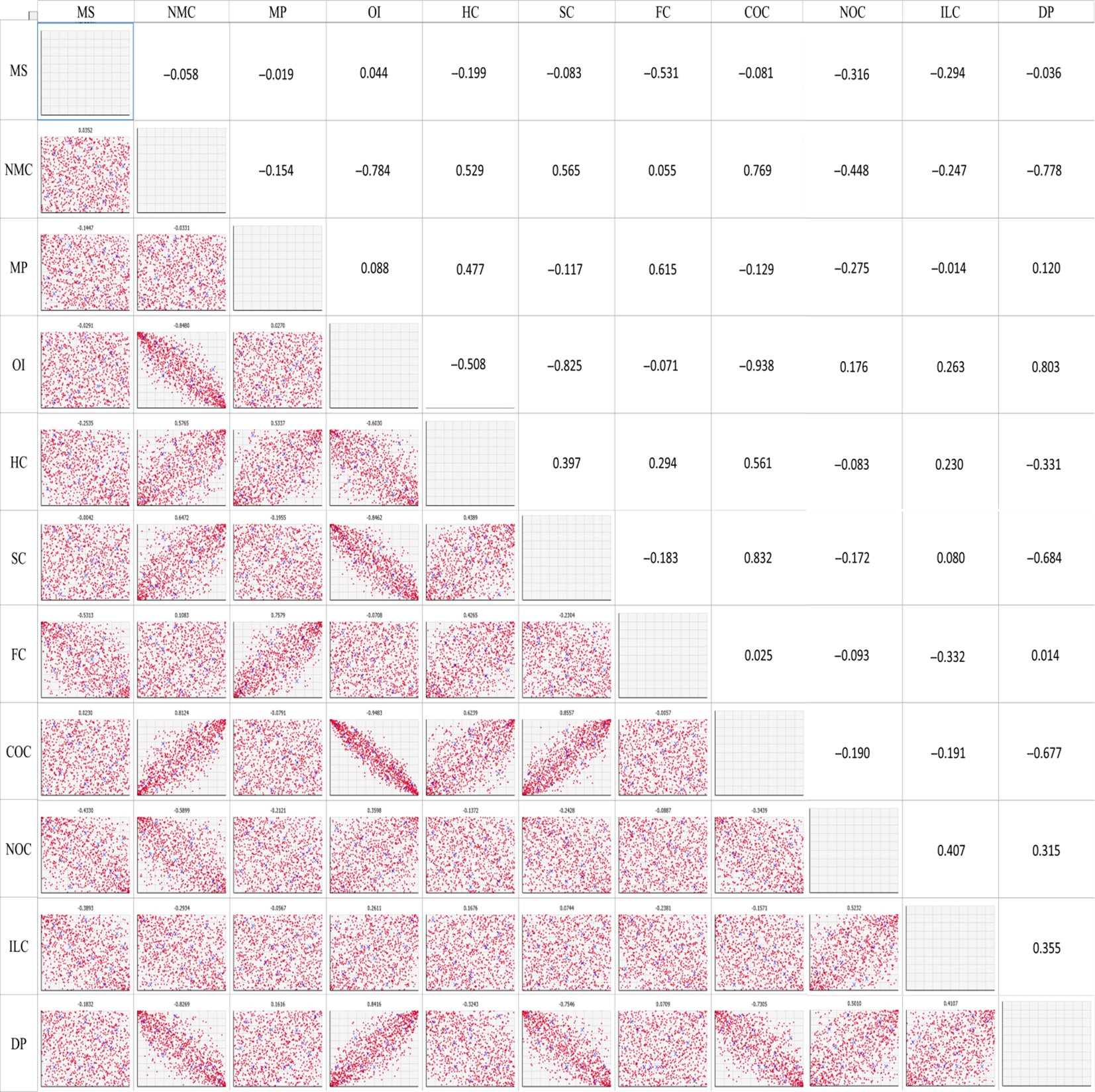
Figure 4. Copula-generated scatter plots (lower triangular cells) and estimated rank correlation matrix (upper triangular cells) used as parameters in the Gaussian copula for the Gippsland (G) Dairy Region. MS: milk sold, NMC: number of milking cows, MP: milk price, OI: other income, HC: herd costs, SC: shed costs, FC: feed costs, COC: cash overhead costs, NOC: non-cash overhead costs, ILC: interests and lease charges, DP: depreciation percentage.

Figure 5. Copula-generated scatter plots (lower triangular cells) and estimated rank correlation matrix (upper triangular cells) used as parameters in the t (df=3) copula for the Southwest (SW) Dairy Region. MS: milk sold, NMC: number of milking cows, MP: milk price, OI: other income, HC: herd costs, SC: shed costs, FC: feed costs, COC: cash overhead costs, NOC: non-cash overhead costs, ILC: interests and lease charges, DP: depreciation percentage.
Table 2. Goodness-of-fit measures for various copula types for the representative dairy region farms of North (N), Gippsland (G), and South West (SW) Victoria
As outlined in Section 2, random variables were generated using the fitted copulae and were converted back to their original scales according to the fitted univariate distributions. These simulated values were then used to drive the profit and loss budgets as well as various performance indices as shown in the sections below.
3.2 Net Farm Income (NP), Sensitivity Analysis, Net Present Value (NPV), and Modified Internal Rate of Return (MIRR)
The representative farms in the North (N), Gippsland (G), and South West (SW) regions of Victoria had opening debts of $1.8m, $1.5m and $1.9m, which at the close of the decade (year 10) had become median debts of $2.6m, $1m and $1.2m, respectively (Table 3). That is, the Northern region median dairy farm debts increased by $0.8m, while Gippsland and South West region dairy farm median debts decreased by $0.5m and $0.7m, respectively.
Table 3. Financial ratios as median values for key performance indicators (KPIs) for the representative Victorian dairy region farm of North (N), Gippsland (G), and South West (SW). All dollar values are in units of thousands
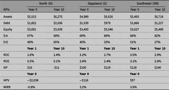
Note: The first five rows of net dollar values compare year zero and year ten. The next three rows compare KPI ratios for year 1 and year 10. The @Risk8.2 model, Monte Carlo simulation, started in year 1 of a randomly drawn decade. The ratios were calculated from @RISK probabilistic output for assets, debt and equity, Earnings before interest and taxation (EBIT) and Net profit (NP). E:A, Equity to Assets ratio; D:A, Debt to Equity ratio; ROC, Return on Capital; ROE, Return on Equity; NP: Net Profit; NPV: Net Present Value; MIRR: Modified Internal Rate of Return.
Business solvency measures of equity to assets ratio per farm at the start of the sample decade in N, G, and SW were 67%, 69%, and 66% and closed at 58%, 84% and 82%, respectively, in year 10. Conversely, median debt to equity ratios per farm at the start of the sample decade in N, G, and SW were 49%, 45%, and 51% and closed at 65%, 25%, and 27%, respectively, in year 10. This is another measure of how much worse the North region has fared than the G and SW.
The median return on capital (ROC) per farm at the start of the sample decade in N, G, and SW were 1.6%, 3.2%, and 3.5% and closed at 1.4%, 2.7%, and 2.9%, respectively, in year 10. Similarly, the median return on equity (ROE) per farm at the start of the decade in N, G, and SW were 0.5%, 2.8%, and 3.1% and closed at 0.1%, 2.4%, and 2.6%, respectively, in year 10.
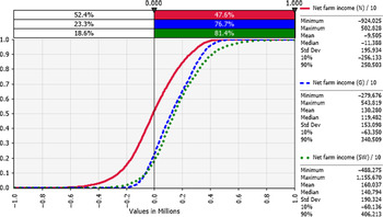
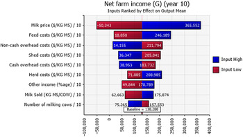
Net farm income was positive 48%, 77%, and 81% of the time for the sample decades for farms in the N, G, and SW regions, respectively (Figure 6). Sensitivity analysis using a tornado graph of mean net farm incomes under the lowest and highest values of input variables (Figures 7–9) showed that the price of milk followed by number of milking cows, feed costs, and non-cash overhead costs, were the key input variables responsible for the largest changes in net farm profits in all three Victorian dairy regions.

Figure 6. Cumulative frequency distributions of net farm income (NP): risk profiles for dairy farms in the N (red), G (blue), and SW (green) regions of Victoria (year 10 of sampled decades), where the y-axis shows the probability of obtaining a value less than or equal to the corresponding x-axis value.
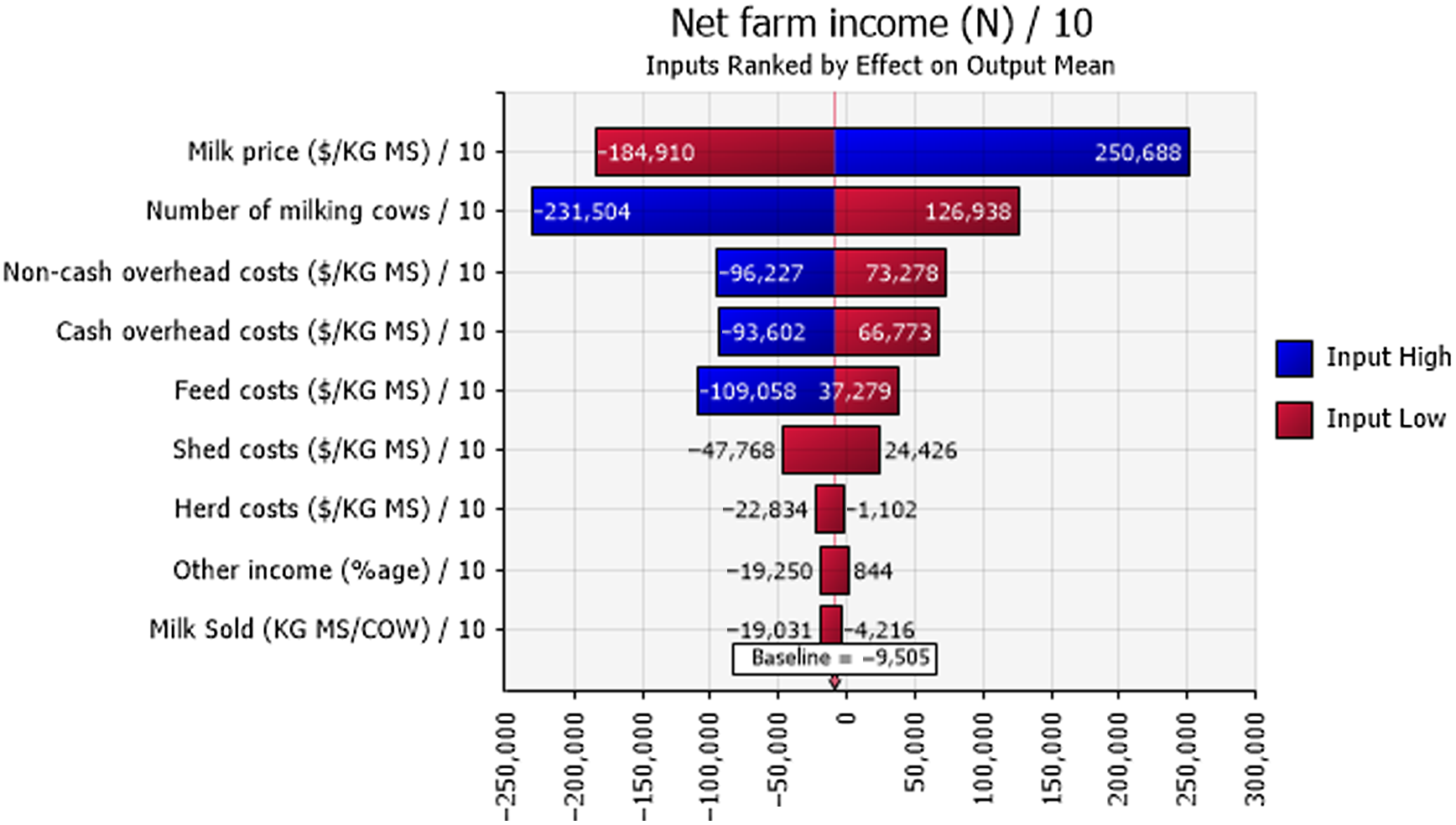
Figure 7. Mean net farm incomes at year 10 at the highest 10% (blue) and lowest 10% (red) of simulated values of input variables in the N region of Victoria. The number at the edge of each bar is the mean net farm income. The “baseline” value is the overall mean net farm income calculated using all simulated values.
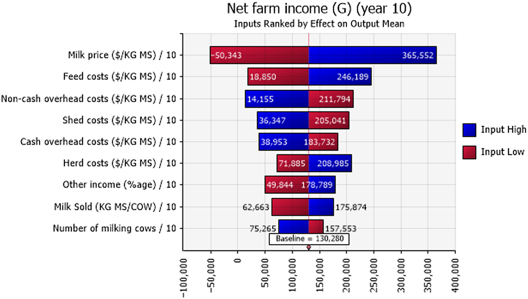
Figure 8. Mean net farm incomes at year 10 at the highest 10% (blue) and lowest 10% (red) of simulated values of input variables in the G region of Victoria. The number at the edge of each bar is the mean net farm income. The “baseline” value is the overall mean net farm income calculated using all simulated values.
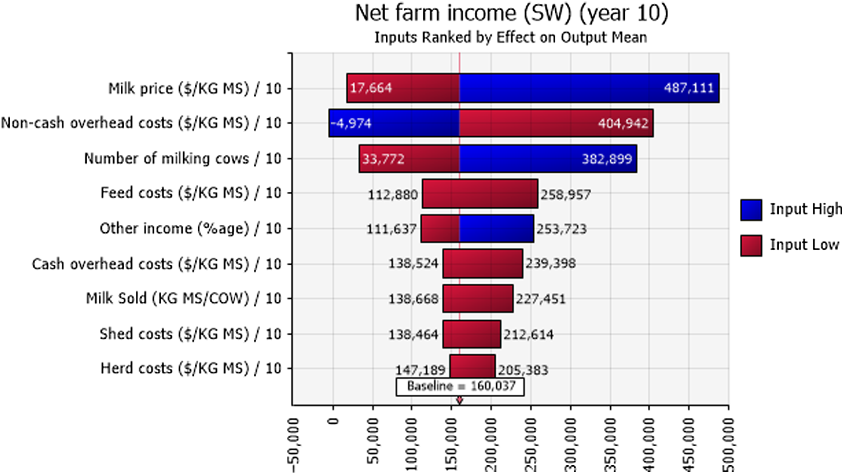
Figure 9. Mean net farm incomes at year 10 at the highest 10% (blue) and lowest 10% (red) of simulated values of input variables in the SW region of Victoria. The number at the edge of each bar is the mean net farm income. The “baseline” value is the overall mean net farm income calculated using all simulated values.
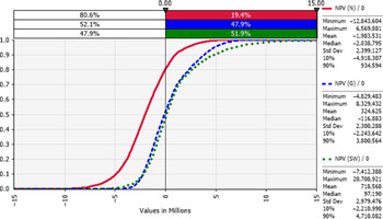
Net present values (NPVs) for the three representative farms were positive 19%, 48%, and 52% for each of the N, G, and SW regions, respectively (Figure 10). Table 3 shows the median modified internal rate of return (MIRR) that was higher than the 4% real hurdle rate of return 15%, 42%, and 45% of the times, respectively, for the three representative Victorian dairy farms.

Figure 10. Cumulative frequency distributions of the net present value (NPV): risk profile for dairy farms in the N (red), G (blue), and SW (green) regions of Victoria (year 0 or opening year), where the y-axis shows the probability of obtaining a value less than or equal to the corresponding x-axis value.
4. Discussion
Our whole-farm dairy business analysis used @RISK8.2 (Palisade Corporation, 2021) and Victorian dairy farm data (Agriculture Victoria and Dairy Australia, 2019) to project a 10-year probabilistic model to understand the business and financial viability of average representative farms in three regions of Victoria. Thirteen-year annual average deterministic inputs of price, production, and cost variables were used in the probabilistic model where the output varied from instance to instance. A major difference between our approach and most, if not all, of the previous Australian dairy farm risk studies is the incorporation of the dependency structure between the input variables through copulae.
Debt, accumulated over time, for the Northern farm is as quantified in Table 3. The Gippsland and South West farms, however, were able to retire debt and ended with a healthier balance sheet than they began with. Our simulation demonstrated that an increase in fixed assets such as land does not help the business if the regular positive stream of income is not there. The farms in all three regions started with different opening debts, but the N region representative farm failed to retire the debt or maintain and increase equity, for reasons discussed earlier.
Farm solvency KPI ratios of equity to assets and debt to equity (Table 3) generated from the financial statement showed the adverse outcome for the N region on both accounts and highlighted that an average representative farm in that region has not fared very well. The N farm’s equity to asset ratio went from being healthy to worsening over the decade as the debt rose. In a real-life situation, the representative farm in the North would have been bankrupt much earlierFootnote 1 , as the increase in farmland value as an asset did not match the compounding impact of debt, that is, the farmer’s liability. Both Gippsland and South West farms ended up with healthier financial statements with an overall increase in the equity to assets ratio. The smaller debt to equity ratio again highlights that there was an increase in equity versus debt for these two regions.
The financial efficiency KPI measure of return on capital (ROC) invested (Table 3) was captured by the smaller ratio in year 10 for all three regions, reflecting the land value appreciation over the decade. In a non-simulation based study, Heard et al. (Reference Heard, Lawrence, Ho and Malcolm2017) reported a ROC of 6.7% across the state of Victoria. However, with potentially non-linear dependency between the input variables taken into account, our results have shown a much lower return, exemplifying the risk of ignoring the dependency structure among input variables. The return on equity (ROE) represented a larger closing ratio for the N region due to a decrease in equity over time. The situation was much healthier for the G and SW regions, their smaller ratios indicating increased owner’s equity.
The probabilistic net farm income or profitability profiles (Figure 6) generated from the historical data showed the North region to be worst off, followed by Gippsland and then South West, which is in better shape. The profitability impacted the balance sheet and NPVs. In all three regions, the largest factor impacting the profitability was the price of milk (Figures 7–9). The difference in average net farm income at year 10 was more than $400,000 between the lowest and the highest 10% of milk price. Other influential factors include number of milking cows, feed costs as well as non-cash overhead costs (Figures 7–9). A recent development, that is, the introduction of a mandatory code of conduct (ABC Landline, 2020) in the way farmers and processors do business, may provide much needed security and some stability to the dairy farmers. Until recently, there has been a mass farmer exodus (Dalhsen, Reference Dalhsen2020) following the deregulation of the Australian dairy industry in 2000. The Department of Agriculture Victoria and Dairy Australia (2019) cost data are detailed and can be dissected further to understand the impact of a range of variable inputs, including different costs impacting net farm incomes. In Victoria’s North region, the rising cost of water is another significant factor adding further burdens to many farmers, particularly during the recent droughts.
The net present value (NPV) at the real discount or hurdle rate of 4% for these three scenarios presented a similar story (Figure 10). The North representative farm was worse off, due to reduced water supplies amid drought and redirection of priority water allocations to environmental use, which explains the mass industry exodus. The modified internal rate of return (MIRR) (Table 3) portrays a similar picture for these farms, particularly in the North, suggesting these farmers consider investing their money elsewhere.
The parameters in the Gaussian or t copula fitted rank correlation matrices demonstrate high degrees of differences in the dependency structures among the variables across the three regions studied (Figures 3–5). For example, milk sold was found to be moderately to strongly correlated with other income, non-cash overhead costs, and interest and lease charges in the North region. However, none of these relationships can be found in the other two regions. Across the three regions, the only common relationships are cash overhead costs and herd costs, and cash overhead costs and shed costs, where moderate to strong positive correlations were found. Naturally, these differences were also reflected when data were simulated from the fitted copulae (Figures 3–5). The differences in the dependency structures may be attributed to some factors which were not considered in the present study. Our work could potentially be extended by incorporating covariates (Alidoost, Stein, and Su, Reference Alidoost, Stein and Su2018). As demonstrated in Ramsey, Goodwin, and Ghosh (Reference Ramsey, Goodwin and Ghosh2019), it may be useful to consider the spatially varying dependence between the input variables in the selection and estimation of the copulae. The recent results in the area of spatial copula models (Krupskii, Huser, and Genton, Reference Krupskii, Huser and Genton2018; Sang and Gelfand, Reference Sang and Gelfand2010) may be useful in further improving our model.
A limitation of this study is the short length of the time series data used. This may have affected the accuracy of the individual univariate distributions, which may have in turn caused biases in the copula parameters (Fantazzini, Reference Fantazzini2009). It is expected that more accurate results can be achieved when longer time series become available. While truncated distributions are often more sensible for agricultural data (e.g., the price of milk cannot be negative), the functionalities in handling truncated distributions are limited in the software used, especially when copulae are involved. Such analyses can be accomplished using other software (Emura and Pan, Reference Emura and Pan2020) but at a higher level of computational complexity.
Disaggregated analyses of individual farms could have revealed the full range of conditions and responses among the district populations. A limitation of this study, owing to our lack of direct access to individual farm records, was due to the requirement of guarding the privacy of the participating businesses. Thus, it is likely that the averaged data used may not truly reflect actual dependency structures amongst input variables. If more detailed data become available, future work could be conducted by applying the same methodology to individual farm data.
Among the copula types considered, it is clear that various measures suggested the use of an elliptical copula for all the three regions (Table 3). One drawback of elliptical copulae is the implicit assumption of symmetric dependence between all variables, which may not always be realistic. It would be interesting to see if the use of some “modern” copula models such as vine copulae (Aas et al., Reference Aas, Czado, Frigessi and Bakken2009; Dißmann et al., Reference Dißmann, Brechmann, Czado and Kurowicka2013), kernel-vine copulae (Zhang and Goodwin, Reference Zhang and Goodwin2020), time series copula models (Patton, Reference Patton2012) may further enhance the results—a direction for future research.
Another limitation of this model-based study, however, is the assumption that conditions from the past will continue in future, which often may not be the case. Also, many factors can impact the industry, such as floods, fires, the COVID-19 outbreak or the trade terms for dairy exports, although the model can handle these later scenarios with some added assumptions.
5. Conclusion
The business and financial risks for three dairying regions in Victoria based on variability in production, prices, and costs were captured in this analysis using historical data with @RISK8.2. The method used allows realistic summaries of long-term portfolios of net farm profits, which extends the usefulness of past data by illuminating the business and financial risk profiles with the farmer’s management information.
We have compared representative dairy farms over the 2006–2007 to 2018–2019 period in each of the three dairy regions of Victoria. It is clear that dairy farms in the North have suffered most from low milk prices, increased feed costs, water shortages, and dependencies on the troubled Murray Darling Basin, leaving these businesses, on average, in precarious financial positions. Dairy farms in the Gippsland and South West have fared better, on average, throughout our study, remaining financially viable and able to make adjustments; they received higher rainfalls and suffered fewer feed shortages, in addition to ending at lower levels of outstanding debt for the study period.
Our probabilistic simulation model has dealt with the “flaw of averages” used in a deterministic model that “best-guesses” the input levels for each iteration by incorporating uncertainty explicitly using a simulation model (Albright and Winston, Reference Albright and Winston2019, p. 179) based on the distributions of these input variables (as in Appendix A and Figures 3–5). Our analysis has focused on defining and comparing the differences in the financial performance of representative dairy farms characterized for each of the three main Victorian dairy regions through the turbulent period of 2006–2007 to 2018–2019. These years brought the Global Financial Crisis, drought periods, and the two major food retailers reducing their milk prices to $1 per liter as loss-leaders to entice customers into their stores. This study simply quantifies the changing fortunes of dairy farmers in contrasting physical, economic and financial conditions.
For farmers, our key messages include finding conditions different among regions in terms of physical production potentials, changing rules limiting access to water in one region, resulting in high feed costs. The results of these factors combined with rainfall variations were captured in terms of financial outcomes over time, showing dairies in one district to be on strong business footings and those in another district to be failing businesses. For analysts, the results in this paper have shown that, when simulating financial outcomes, it is vital to consider dependence among variables.
Acknowledgements
We are indebted to the Graham Centre for Agricultural Innovation for supporting this work. An earlier version of the present paper was presented at the AARES conference in Perth in February 2020 (Godfrey et al., Reference Godfrey, Nordblom, Ip and Hutchings2020). We note that Dairy Australia and Agriculture Victoria used methods adapted from The Farming Game (Malcolm, Makeham, and Wright, Reference Malcolm, Makeham and Wright2005) in developing their detailed Dairy Farm Monitor Project, which was the key data source for this paper. The authors alone are responsible for any errors in this study. The authors thank the reviewers for their constructive comments.
Author contributions
Conceptualization, S.S.G., T.L.N., R.H.L.I. ; Methodology, S.S.G., R.H.L.I. and T.L.N.; Formal Analysis, S.S.G and R.H.L.I.; Data Curation, S.S.G. ; Writing—Original Draft, S.S.G., T.L.N. and R.H.L.I., Writing—Review and Editing, S.S.G., R.H.L.I. and T.L.N.
Financial support
This research received no specific grant from any funding agency, commercial or not-for-profit sectors.
Conflict of interest
Authors Sosheel Solomon Godfrey, Ryan H. L. Ip and Thomas Lee Nordblom declare none.
Data availability statement
The Dairy Farm Monitor Project (DFMP) data analyzed in this project is open access and available using the links below:
https://agriculture.vic.gov.au/about/agriculture-in-victoria/dairy-farm-monitor-project
Appendix A: Fitted Univariate Distributions
Table A1. Fitted univariate distributions for the input variables (and the theoretical summary statistics) for North (N) dairy region
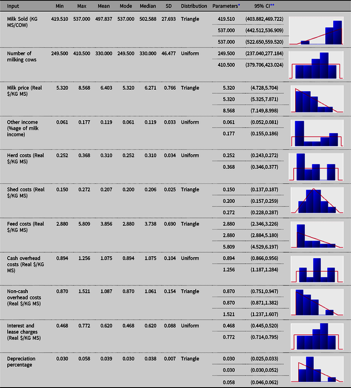
Table A2. Fitted univariate distributions for the input variables (and the theoretical summary statistics) for Gippsland (G) dairy region
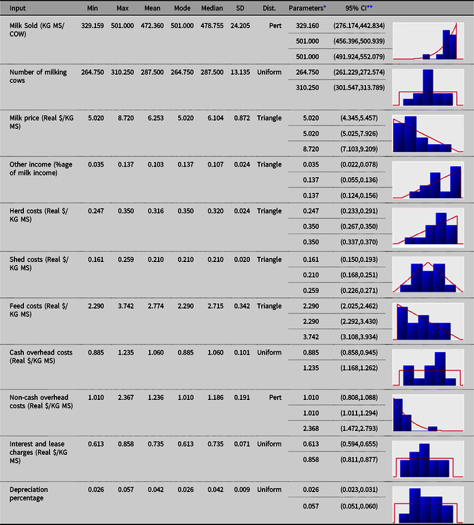
Table A3. Fitted univariate distributions for the input variables (and the theoretical summary statistics) for Southwest (SW) dairy region


 Open access