


Introduction
Futures contracts on storable commodities reflect price expectations based on information regarding inventories (Working, Reference Working1948). However, they cannot reflect the level of uncertainty that the market associates with these price expectations. Implied volatility (IV), on the other hand, measures the degree of uncertainty the market puts on the futures price at the expiration of the option contract and can be regarded as a forward-looking measure of volatility (McNew and Espinosa, Reference McNew and Espinosa1994). Furthermore, IV is shown to better predict realised volatility, which is backward-looking (Guo, Han, and Zhao, Reference Guo, Han and Zhao2014; Haugom et al., Reference Haugom, Langeland, Molnár and Westgaard2014; Mixon, Reference Mixon2002; Szakmary et al., Reference Szakmary, Ors, Kim and Davidson2003). Understanding the determinants of IV is important to both agricultural policy makers and market participants. The Risk Management Agency (RMA) of the United States Department of Agriculture (USDA) also uses IV as a market-based measure of expected prices’ variability in determining premium rates in crop revenue insurance for major commodities. A better knowledge of future uncertainty levels is also important for determining effective hedge ratios and managing risks with temporal dimensions (Egelkraut, Garcia, and Sherrick, Reference Egelkraut, Garcia and Sherrick2007). Consequently, market uncertainty levels, including IV, serve as important benchmarks or indicators in largely volatile food commodity markets, where price variability and supply-demand shocks are closely related.
Our paper aims to shed light on the determinants of volatility measures, especially the forward-looking IV. To this end, we turn our attention to the impact of fundamentals on volatilities in futures and options markets for substitutable agricultural commodities, while controlling for other factors that are shown to affect volatility. Since some agricultural commodities are characterised as production or economic substitutes for each other, we focus not only on the own market’s fundamentals but also on the spillover effects of substitute commodity fundamentals.
During the commodity price boom of 2007–2008, higher volatility of global food prices became an even greater concern. Some blamed commodity index funds for putting speculative pressure on food prices, while a more commonly accepted reasoning was the increase in food demand from developing countries. This increased demand drove inventories to low levels, causing spikes in storable commodity prices (Beckmann and Czudaj, Reference Beckmann and Czudaj2014; Carpentier and Dufays, Reference Carpentier and Dufays2013; Carter, Rausser, and Smith, Reference Carter, Rausser and Smith2011; Wright, Reference Wright2011). The prevalent economic crisis and linkages among commodity prices during that period worsened the impact of shocks to fundamentals in storable commodity markets.
The extant literature investigates the nexus between price volatility, defined as the day-to-day percentage change in a commodity price, and storage regimes, while few prior studies explore the link between IV and storage (Adjemian et al., Reference Adjemian, Bruno, Robe and Wallen2017; Litzenberger and Rabinowitz, Reference Litzenberger and Rabinowitz1995; Robe and Wallen, Reference Robe and Wallen2016). Determining similar drivers of a forward-looking volatility measure is important for assessing the relative costs and risks of hedging for various market participants. As IV anticipates realised volatility better than historical information, market participants can use the information content of IV in developing better trading strategies.
Storage plays a shock-absorbing role in commodity markets against the predictable components of fluctuations in supply and demand. Further, when inventories are low, the size of commodity futures price changes, another measure of volatility, in response to demand/supply or information shocks is large (see Thurman Reference Thurman1988; Karali and Thurman, Reference Karali and Thurman2009; Williams and Wright, Reference Williams and Wright1991; and Karali, Reference Karali2011). Thus, storage has a moderating influence on both current and future uncertainty. In our study, we adopt a measure of storage that captures the future state of inventories. Economic theory suggests that the future price of a storable commodity should be equal to the current spot price plus the cost of storage, including interest charges and risk premium. In practice, however, spot prices might exceed nearby futures prices, or near-delivery futures prices might exceed far-delivery futures prices (Working, Reference Working1933, Reference Working1948). This phenomenon is known as the “inverted market” and can occur due to “convenience yield” generated as an embedded option value, that is, an implied benefit accrued from the physical storage of commodities (Joseph, Irwin, and Garcia, Reference Joseph, Irwin and Garcia2016; Kaldor, Reference Kaldor1939; Paul, Reference Paul1970; Telser, Reference Telser1958; Working, Reference Working1949). The opposite price pattern, in which more distant prices exceed nearby prices, is called the “normal market.” In many previous studies, the term “backwardation” has been interchangeably used for an inverted market and “contango” for a normal market.Footnote 1 We adopt this terminology to align with the literature. To analyse the link between the forward-looking volatility measure (IV) and storage, we proxy inventory conditions by price-based, forward-looking net cost of carry, calculated from different-delivery futures contract prices. This empirical relationship between storage and the intertemporal price differences (i.e., the Working curve) represents a forward-looking measure of the inventory situation in commodity markets.
Few studies establish the role of commodity-related fundamentals as key determinants of IV. Litzenberger and Rabinowitz (Reference Litzenberger and Rabinowitz1995) show that oil production is inversely related to IV, while backwardation is positively related. Robe and Wallen (Reference Robe and Wallen2016) find that the relation between crude oil IV and the slope of the futures term structure (represented by the ratio of deferred futures price to nearby futures price) is stronger in periods of contango compared to the periods of backwardation. For grain markets, Adjemian et al. (Reference Adjemian, Bruno, Robe and Wallen2017) establish that near-stockouts tend to boost nearby IV, whereas high inventories reduce it. The differential impact of the state of inventories on oil versus grain IV is likely associated with the fact that oil production is continuous throughout the year in contrast to the seasonal production of grains. IV patterns in grain markets should also reflect seasonal patterns in production. For example, uncertainty in grain markets should be high during the summer months when adverse weather might cause a shortage in supply. Our work builds upon these previous studies and facts to investigate how the IV dynamics depend on commodity fundamentals as well as macroeconomic and financial market indicators in grain and oilseed markets. We further extend the previous work by studying potential spillover effects across substitute commodity markets on both the nearby and deferred IV patterns.
In the U.S., corn and soybean are close substitutes in production and their growing areas overlap, specifically across the Corn Belt. Producers make planting decisions based on the corn-to-soybean price ratio, which is one of the many measures used to ascertain the profitability of corn and soybean (Taylor and Koo, Reference Taylor and Koo2010). As a result, they both compete for storage space where the supply of storage for corn (soybean) can be reduced due to higher inventories/production of soybean (corn) (Liu, Reference Liu1983). The overlapping production areas also indicate that the impact of weather shocks on production is highly correlated for corn and soybean. Similarly, the impact of shocks to transportation, which would affect the derived demand for corn and soybean, should also be correlated in these two markets. Therefore, it is reasonable to expect production surprises and/or supply disruptions in one market to drive price reactions in the other market. In fact, soybean futures prices, for example, are shown to be sensitive to production surprises in the corn market (Karali et al., Reference Karali, Isengildina-Massa, Irwin, Adjemian and Johansson2019).
Hard red winter (HRW) wheat and hard red spring (HRS) wheat belong to hard wheat classes, where substitution elasticities indicate that winter and spring wheat types are economic substitutes for milling purposes (Marsh, Reference Marsh2005). Moreover, HRW wheat accounts for 40% of U.S. wheat production, which makes it the largest wheat class in the U.S.Footnote 2 As a result, a bad crop year resulting in low inventories of winter wheat will put pressure on producers to increase spring wheat production to meet the demand of domestic flour millers for the high protein hard wheat class. Wilson (Reference Wilson1983) also establishes the dominant role of commodity-specific fundamentals in determining the price relationships between the two classes of wheat. Therefore, one should account for possible spillover effects across commodity fundamentals while determining the underlying factors affecting the IV series of substitute wheat varieties.
Our approach enables studying grain and oilseed IV patterns in the context of substitute commodity markets, where apart from the own fundamentals we expect the substitute commodity fundamentals to impact the IV series while controlling for other macroeconomic and financial market indicators. Specifically, we analyse the impact of physical commodity measures, such as inventory conditions proxied by backwardation and contango and stocks-to-use ratio, on the forward-looking measure of price variability (i.e., IV) in both own and substitute commodity markets. This reconciles our approach with the literature that emphasises the impact of underlying supply and demand-related factors on both backward-looking and forward-looking measures of price variability in the grain markets.
We adopt the methodology of Goodwin and Schnepf (Reference Goodwin and Schnepf2000), who investigate the impact of various factors including growing conditions and stocks-to-use ratios on both futures price variability and volatility implied in the options market. Their study finds strong impacts of shocks to growing conditions on IV series of corn and spring wheat, but a modest impact of stocks-to-use ratios. However, our study’s premise to include storage regimes—as determinants of expected-price variability—is that extreme events in the form of glut (also referred to as contango) or stock-outs (also referred to as backwardation) should heighten volatilities derived from options as the uncertainty related to commodity fundamentals increases. For example, inventory conditions indicating a glut in the corn market are likely to increase the demand for storage—with the supply of storage relatively constant—therefore, spiking future uncertainty levels. Likewise, stock-outs in hard wheat markets can spike future uncertainty levels in the commodity markets as HRW and HRS are the mainstays of the domestic U.S. flour market.
Across our nearby- and deferred-contract analyses, we show some evidence of both own and spillover effects of storage regimes on futures return variances and IVs in the U.S. grain and oilseeds markets. We find modest spillovers from storage regimes in the substitute commodity market to impact futures and options-derived volatilities of a crop, whereas own market’s storage regimes have stronger impacts. While the market-wide volatility index has a significant impact in all markets but winter wheat, our results demonstrate that it cannot be the sole determinant of volatilities in grain and oilseeds markets and both own and substitute commodity fundamentals should be considered to accurately portray IV patterns.
Empirical Model
Following Goodwin and Schnepf (Reference Goodwin and Schnepf2000), we investigate the factors affecting commodity price variability through a couple of different econometric approaches. Given that IVs are derived from futures prices, we first analyse the futures return in each market by modelling its variance through both a conditional heteroskedasticity (CH) model and a generalised autoregressive heteroskedasticity (GARCH) model. Then, employing a GARCH framework we focus on the determinants of the IV series. Finally, we estimate a nonstructural vector autoregressive (VAR) model for each IV series to evaluate their dynamic relationships with a subset of variables that affect price volatility.
CH Model of Futures Returns
Futures return for each commodity can be specified as:
 $$R_{t}=\mu +X_{t}\delta +\epsilon _{t},$$
where R
t
= 100 × (lnP
t
−lnP
t − 1) is the continuously compounded daily return on the futures contract with price P
t
on day t, X
t
is the vector of independent variables, including lagged futures returns to account for serial correlation and commodity fundamentals in both own and substitute market (net cost of carry during contango and backwardation, stocks-to-use ratio), δ is the parameter vector, and ϵ
t
is the error term with zero mean and variance of ${\rm Var}(\epsilon _{t})=\sigma _{t}^{2}=f(Z_{t}\theta )$
. Thus, the variance of futures returns depends on a set of explanatory variables Z
t
. As the error term is unobservable, the estimated residuals from equation (1),
${\rm Var}(\epsilon _{t})=\sigma _{t}^{2}=f(Z_{t}\theta )$
. Thus, the variance of futures returns depends on a set of explanatory variables Z
t
. As the error term is unobservable, the estimated residuals from equation (1), ${\hat\epsilon}_{t}^{2}$
, can be used to form the following CH model (Harvey, Reference Harvey1976):
${\hat\epsilon}_{t}^{2}$
, can be used to form the following CH model (Harvey, Reference Harvey1976):
 $$\ln \hat{\epsilon }_{t}^{2}=Z_{t}\theta +\nu _{t},$$
where θ is the parameter vector and ν
t
is the error term with zero mean and constant variance. This formulation helps us model heteroskedasticity in line with the general multiplicative heteroskedasticity models. The explanatory variables in (2) include an intercept, lagged variances of returns (i.e., lags of ln ${\hat\epsilon}_{t}^{2}$
to account for serial correlation), commodity fundamentals in both own and substitute market (net cost of carry during contango and backwardation, stocks-to-use ratio), dummies for crop planning/planting and preharvest seasons, financial market indicator (volatility index—VIX), macroeconomic indicator (Hamilton index), time-to-maturity (TTM), contract roll dummy and a dummy for the 2007–2008 economic crisis.
${\hat\epsilon}_{t}^{2}$
to account for serial correlation), commodity fundamentals in both own and substitute market (net cost of carry during contango and backwardation, stocks-to-use ratio), dummies for crop planning/planting and preharvest seasons, financial market indicator (volatility index—VIX), macroeconomic indicator (Hamilton index), time-to-maturity (TTM), contract roll dummy and a dummy for the 2007–2008 economic crisis.
GARCH-X Model of Futures Returns
We also employ a GARCH-X(1,1) framework with multiplicative heteroskedasticity for modelling futures return variance as shown below:
 $${\rm Var}\left(\epsilon _{t}\right)=\sigma _{t}^{2}=\alpha \epsilon _{t-1}^{2}+\beta \sigma _{t-1}^{2}+\exp (Z_{t}\theta ),$$
where α and β are ARCH and GARCH parameters, respectively, and the vector Z t contains the same explanatory variables as in equation (2).
GARCH Model of IV Series
Because IV series exhibit ARCH effects based on the Lagrange Multiplier test, we model each IV series with the error variance specified by a simple GARCH(1,1) framework:
 $${\rm IV}_{t}=\phi +H_{t}\gamma +\varepsilon _{t},$$
 $${\rm Var}\left(\varepsilon _{t}\right)=\sigma _{t}^{*2}=\omega +\alpha ^{*}\varepsilon _{t-1}^{2}+\beta ^{*}\sigma _{t-1}^{*2},$$
where H t is the vector of explanatory variables, including lagged IVs to account for serial correlation, commodity fundamentals in both own and substitute market (net cost of carry in contango and backwardation, stocks-to-use ratio), dummies for crop planning/planting and preharvest seasons, financial market indicators (VIX and options hedging pressure), macroeconomic indicator (Hamilton index), TTM, contract roll dummy and a dummy for the 2007–2008 economic crisis. The parameters ω, α* and β* in (5) represent the constant conditional volatility, ARCH and GARCH effects, respectively.
Vector Autoregressive Model and Impulse Response Functions
Similar to Goodwin and Schnepf (Reference Goodwin and Schnepf2000), we estimate a ten-equation nonstructural vector autoregressive (VAR) model for each IV series to evaluate their dynamic relationships with a subset of variables (commodity fundamentals in both own and substitute market, hedging pressure in own market, and VIX) that affect futures price volatility. Each of these VAR models also contains as exogenous factors the Hamilton index, TTM, dummy variables for crop planning/planting and preharvest seasons, contract rollover dummy, and a dummy for the 2007–2008 economic crisis. We illustrate the adjustment paths of implied volatility to shocks in those other variables using orthogonalised impulse response function (IRF) analysis.
Data
Our sample period spans from 1996 to 2019. In the following, we describe in detail all variables used in our analysis.
Futures and IV Series
We use daily data on futures prices and IV series obtained from Barchart (formerly, the Commodity Research Bureau).Footnote 3 Corn, soybean and hard red winter (HRW) wheat contracts are traded at the Chicago Mercantile Exchange (CME) Group, and hard red spring (HRS) wheat contracts are traded at the Minneapolis Grain Exchange (MGEX). Futures contracts of the selected commodities expire on the business day preceding the 15th day of the maturity month, and the associated options contracts terminate a few days prior to the futures contracts’ delivery period. To avoid the impact of the delivery process, we roll over these contracts on the 15th calendar day of the month prior to maturity.Footnote 4 Table 1 lists the specific contracts we use to construct nearby futures and IV series for our analysis. In our empirical models, we include a dummy variable indicating contract rollovers to account for possible jumps in volatility when one switches from one contract to the next.
Table 1. Futures and options contracts rollover

Descriptive statistics in Table 2 show that daily nearby futures returns and IV series are leptokurtic; that is, they have fatter tails than a normal distribution. This is in line with the previous literature on agricultural commodity markets (Hall, Brorsen, and Irwin, Reference Hall, Brorsen and Irwin1989; Koekebakker and Lien, Reference Koekebakker and Lien2004). Further, Lagrange Multiplier tests confirm heteroskedasticity in both futures returns and IV series; thus, making a case for a GARCH model.Footnote 5
Table 2. Descriptive statistics
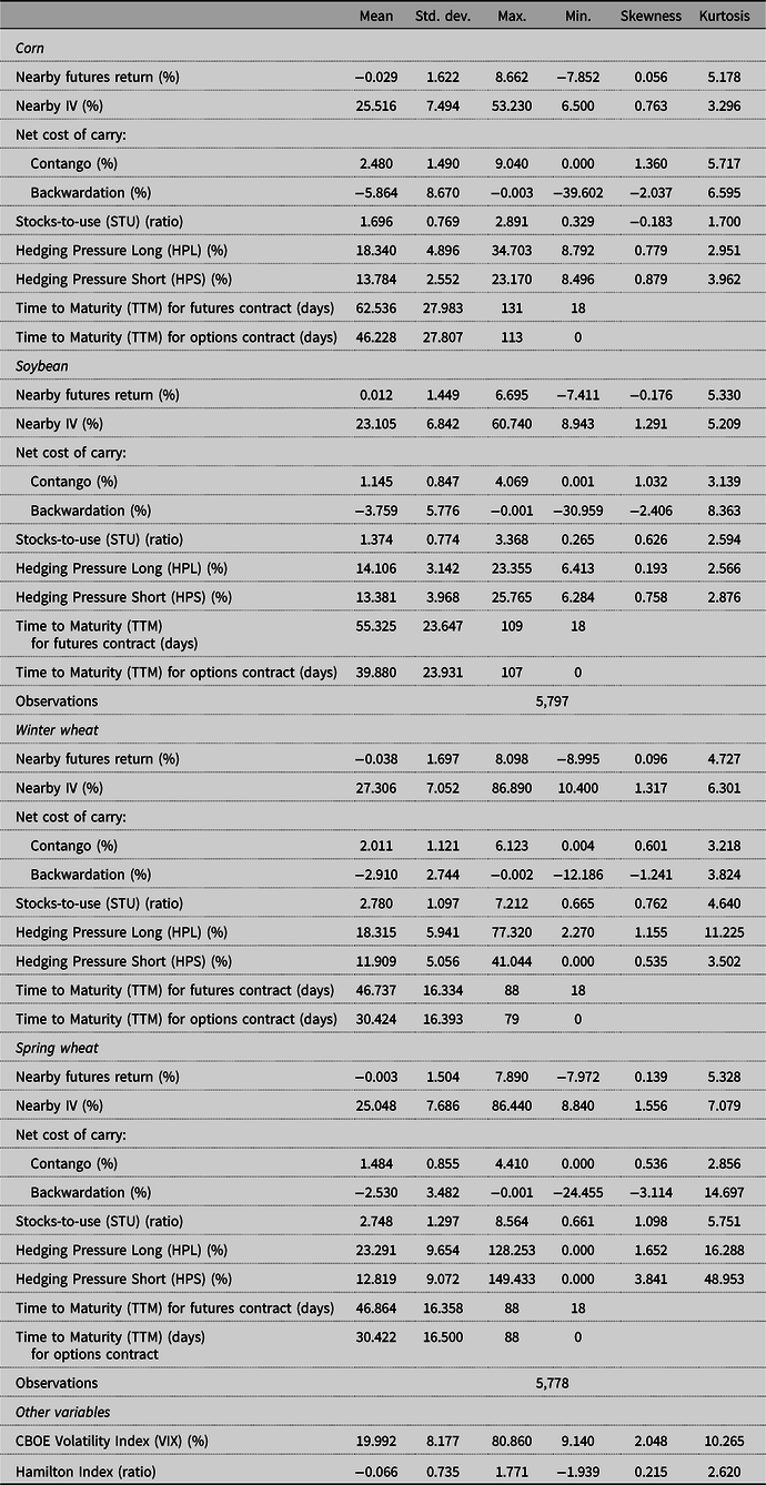
Note: Sample period is from 1996 to 2019. All variables, except for stock-to-use ratios and hedging pressures, are measured at the daily frequency. Net cost of carry per bushel is calculated using the nearby and 1st deferred futures series to indicate the slope of the term structure. The coefficient for skewness is m 3 m 2 −3/2 and for kurtosis is m 4 m 2 −2, where m r is the r th moment about the mean.
Futures contracts with different maturities can contribute to price discovery in a dissimilar way. For instance, in the corn futures market, nearby contracts reflect information more quickly than deferred contracts (Hu et al., Reference Hu, Mallory, Serra and Garcia2020). Short-term price fluctuations—due to temporary shifts in supply or demand—are less likely to persist for long periods of time before the prices return to their fundamental values (Koekebakker and Lien, Reference Koekebakker and Lien2004). Further, Samuelson (Reference Samuelson1965) asserts that the variance of futures prices increases as the contracts approach delivery, suggesting that short-dated contracts have higher volatility relative to long-dated contracts. This assertion has been viewed as a hypothesis stating more information flows into the markets, and therefore, more uncertainty gets resolved as delivery approaches (Anderson and Danthine, Reference Anderson and Danthine1983; Samuelson, Reference Samuelson1976). To investigate this hypothesis, we also perform our analysis for two deferred futures returns and IV series for each commodity. On average, the first deferred IV series are approximately three months out relative to the nearby contracts, while the second deferred IV series is about five months out. The specific contracts in constructing these deferred series are presented in the appendix Table A1 and their descriptive statistics in Table A2. Consistent with Samuelson’s assertion, the standard deviations of futures returns and IV levels of deferred series are relatively lower than those of nearby series for all commodities.
Commodity Fundamentals
We analyse the impact of commodity fundamentals, both in the own market and in the substitute commodity market, on price variability using two measures of fundamentals. We represent inventory conditions by the net cost of carry calculated using the futures prices. Specifically, we take the difference between the log prices of deferred and nearby futures series less the appropriately adjusted Libor rate and multiply the result by 100 to state the net cost of carry in percentage terms.Footnote 6 We then interact the net cost of carry with dummy variables indicating contango (i.e., net cost of carry greater than or equal to zero) and backwardation (i.e., net cost of carry less than zero) to distinguish carrying costs during these two storage regimes. The carrying cost of a commodity during an episode of low inventories in the own market should heighten the volatility levels, while an episode of plentiful inventories should reduce volatility given that the rather constant storage supply satisfies the demand for commodity storage. Hence, we expect a negative sign for the net cost of carry for a given commodity during both contango and backwardation in its own market.Footnote 7 Table 2 shows that, in absolute terms, the net cost of carry in contango is lower than the net cost of carry in backwardation in all four commodity markets.
To study the impact of supply and demand-side factors, we use USDA’s quarterly estimates for ending stocks and use (or disappearance).Footnote 8 The ratio of ending stocks to use, our STU variable, captures the impact of higher or lower levels of inventories relative to a given level of demand for the current crop year on the two measures of price variability: futures return variance and IV. Since options are written on underlying futures contracts, any discontinuities due to supply or demand-side disruptions should affect both futures and options markets (Koekebakker and Lien, Reference Koekebakker and Lien2004). We expect a negative relationship between the STU variable and price variability measures for a given commodity as lower STU ratios indicate higher levels of demand relative to stock levels, signalling a shortage and an upward pressure on prices and their variability.
Seasonality and Time-to-Maturity
Volatility in futures returns is a function of seasonal effects and maturity effects (Galloway and Kolb, Reference Galloway and Kolb1996; Koekebakker and Lien, Reference Koekebakker and Lien2004). To account for seasonality in our econometric approach, we include dummy variables representing planning/planting and preharvest periods, with the postharvest period taken as the base category. We determine these periods based on the Crop Progress reports published weekly by NASS during the growing season (Karali, Dorfman, and Thurman, Reference Karali, Dorfman and Thurman2010). Specifically, we define the planning/planting period dummy as December through May for corn, December through June for soybean, September through November for HRW wheat and October through May for HRS wheat. The preharvest dummy covers the months of June through August for corn, July through August for soybean, December through May for HRW wheat and June through July for HRS wheat. The remaining calendar months for each commodity represent the postharvest period.
TTM, or the Samuelson hypothesis, has been shown in the literature to affect futures price volatility, with volatility increasing as the time to contract expiration nears (Anderson and Danthine, Reference Anderson and Danthine1983; Anderson, Reference Anderson1985; Black and Tonks, Reference Black and Tonks2000; Chatrath, Adrangi, and Dhanda, Reference Chatrath, Adrangi and Dhanda2002; Leistikow, Reference Leistikow1989; Milonas, Reference Milonas1986; Smith, Reference Smith2005). We account for the Samuelson effect by including TTM variables, measured as the number of trading days left to contract expiration, in our empirical models.Footnote 9
Financial Indicators
The use of new generation grain contracts (NGGCs), which establish prescribed rules for pricing grain that will be automatically executed, is slowly gaining traction in the grain markets as producers opt for them as their preharvest strategy to reduce production risk (Elliott et al., Reference Elliott, Elliott, Slaa and Wang2020).Footnote 10 The pricing of insurance in structured products, such as NGGC, relies heavily on the measures of IV. In this context, determining the information content of the implied volatility functions (IVFs) in the commodity markets is of importance to market participants.Footnote 11 Goodwin (Reference Goodwin2015) points out the prevalence of anomalies in the shape of corn IVs—termed as smiles or smirks. The presence of these shapes goes against the assumptions of Black and Scholes (Reference Black and Scholes1973) model that warrants IVFs to be flat over time. Given the importance of IVs as crucial benchmarks for various risk management efforts—be it pricing of crop insurance by RMA or designing of structured products—understanding the determinants of the anomalies such as smirks in IVs can provide insights valuable to both public and private insurance markets. Empirical evidence suggests in the case of S&P 500 options, hedging pressures derived from heterogeneous beliefs of market traders account for smiles or smirks in options prices (Bollen and Whaley, Reference Bollen and Whaley2004; Buraschi and Jiltsov, Reference Buraschi and Jiltsov2006).
In our study, we also control for these heterogeneous beliefs of market traders in the options markets by following the approach in McKenzie, Thomsen, and Adjemian (Reference McKenzie, Thomsen and Adjemian2022). These authors use short-term hedging pressure proxies, calculated using the Commodity Futures Trading Commission (CFTC) reports, to account for the possibility of market-induced pressures impacting the shape of IVFs in cattle and grain markets.Footnote 12 We use both CFTC’s futures only and futures and options combined legacy Commitment of Traders (COT) reports, which are publicly available only on Tuesdays, to construct short-term hedging pressure proxies.
Specifically, we calculate options hedging open interest by taking the difference between the short (long) commercial open interest in both futures and options combined, and the short (long) commercial open interest in futures only. Similarly, we calculate the total options open interest as the difference between the total open interest in the combined reports and the futures-only report.Footnote 13 Before making these calculations, following Kim (Reference Kim2015), Sanders, Irwin, and Merrin (Reference Sanders, Irwin and Merrin2010), and Bohl and Sulewski (Reference Bohl and Sulewski2019), we assume that nonreporting traders exhibit the same distribution pattern as the reporting traders. Accordingly, we allocate nonreporting short and long open interests to commercials and noncommercials contingent upon the ratio of short and long positions held in the reported groups. Next, we calculate our hedging pressure proxies as short-hedging pressure (HPS) and long-hedging pressure (HPL). HPS (or HPL) is taken as the ratio of short (or long) options hedging open interest held by commercial hedgers divided by total options open interest held by all trader groups. According to McKenzie, Thomsen, and Adjemian (Reference McKenzie, Thomsen and Adjemian2022), a higher percentage of HPS suggests higher demand for long puts to manage expected downside price risk, while a higher percentage of HPL suggests higher demand for long calls to manage the upside price risk. In both scenarios, the hedging pressures can induce risk premium in options. We include these two hedging pressure measures of a commodity as explanatory variables in our IV regressions to study their effects in the own market. For all our commodities, we notice relatively higher percentages of HPL in comparison to HPS (Table 2). This suggests a tendency of traders to expect more of an upside price risk in these grain and oilseed markets.
We include the Chicago Board Options Exchange’s Volatility Index (VIX) obtained from Bloomberg as an explanatory variable to study its impact on both measures of price volatility. VIX captures both uncertainty and risk aversion in stock as well as oil markets (Bekaert, Hoerova, and Duca, Reference Bekaert, Hoerova and Duca2013; Robe and Wallen, Reference Robe and Wallen2016) and has been used in the literature (for both stock markets and commodity futures/options) to serve as a ‘fear factor measure’ while accounting for investor sentiments (Adjemian et al., Reference Adjemian, Bruno, Robe and Wallen2017; Whaley, Reference Whaley2000). Based on the study of Adjemian et al. (Reference Adjemian, Bruno, Robe and Wallen2017) on the IV determinants in commodity markets, we expect increases in daily VIX to drive up the uncertainty in our selected markets.
Macroeconomic Indicators
We use a daily series of global economic activity index suggested by Hamilton (Reference Hamilton2021) to replicate world business cycles, which is found to perform better than the Kilian index.Footnote 14 Specifically, we utilise the Baltic Dry Index (BDI) of shipping costs, acquired from Bloomberg, and construct the Hamilton index using differencing instead of detrending. During our sample period, the Hamilton index is negative on average (Table 2). We expect a negative sign for this variable’s coefficient as a downward trend in world business cycles should boost futures return variances and IVs, whereas a positive change should bring them down.Footnote 15 In addition, we account for the global financial crisis of 2007–2008 by including a dummy variable.
Results
The results for corn, soybean, winter wheat and spring wheat nearby futures and IV series are presented in Tables 3 through 6, respectively. To conserve space, we present the results for the deferred series in appendix Tables A3–A10. In each of these tables, panel A shows the mean equation parameters,Footnote 16 whereas panel B presents the variance equation parameters. In our discussion of results, we consider a parameter statistically significant at the 1% level to have a strong impact, a parameter significant at 5% to have a modest impact and a parameter significant at the 10% level to have a weak impact.
Table 3. Determinants of corn nearby volatility

Note: Robust standard errors are given in parentheses. The GARCH-X(1,1) model for futures returns assumes a Student’s t-distribution for the error term and the associated degrees of freedom parameter is estimated along with the other parameters of the model. AIC stands for Akaike’s Information Criteria and BIC stands for Bayesian Information Criteria. The asterisks *, ** and *** represent statistical significance at the 10%, 5% and 1% level, respectively.
Corn
The estimates of the CH model as well as that of the GARCH model for corn futures returns confirm the impact of both corn and soybean fundamentals, indicating spillover effects from the substitute commodity market (Table 3). We find strong negative impacts of corn market’s contango on the mean return levels (−0.053 in the CH model) in contrast to its strong positive impact on the variability of futures returns (0.154 in the GARCH model). The GARCH model for the IV series also shows a modest positive impact (0.045) of a contango in the corn market on the IV level. This suggests, in line with our expectations, the prospects of high corn inventories in the future have a negative influence on futures returns, but contrary to our hypothesis, the possibility of such a glut heightens the two measures of volatility in its own market. Contango’s significant positive impact on volatility could indicate that under the pressure of excess demand for storage, the corn market experiences higher uncertainty (given constant/limited storage space) as it expects plentiful harvests. Spillovers from soybean backwardation have, on average, a weak to modest impact on the corn futures return levels. A positive sign for soybean backwardation in the mean equations of CH and GARCH models suggests that in expectation of soybean shortage (and the subsequent expected rise in soybean prices), the corn market is likely to witness a drop in the mean return levels as selling soybean will be relatively more profitable.Footnote 17 However, the magnitude of the own-contango impact on mean futures returns (0.053 in the CH model and 0.051 in the GARCH model) is higher than that of spillovers from backwardation in soybean (0.011 in the CH model and 0.014 in the GARCH model). We also find that corn STU for the current crop year has a modest positive impact on the mean futures returns (0.080 in the GARCH model). In line with our expectations and with Goodwin and Schnepf (Reference Goodwin and Schnepf2000) results,Footnote 18 we find a modest to strong negative impact of corn STU on the two measures of price variability (both the variance of futures returns and the IV). This suggests higher levels of current stocks relative to current demand are likely to reduce the variability in corn prices. There is some evidence for spillovers from soybean STU to reduce the variability of corn prices, but the impact is lower in magnitude (0.210 in the CH model) relative to the own STU effect (0.590 in the CH model and 1.070 in the GARCH model).
Among the financial indicators, hedging pressure variables do not show any significant impact on the corn IV, consistent with the findings in McKenzie, Thomsen, and Adjemian (Reference McKenzie, Thomsen and Adjemian2022). On the other hand, CBOE’s VIX has a weak positive impact on the variability of corn futures returns but a strong positive impact on IV. This finding is consistent with Adjemian et al. (Reference Adjemian, Bruno, Robe and Wallen2017). The strong impact of the Hamilton index is evident in the variance equations of futures return models, while the 2007−2008 economic crisis consistently shows a strong positive impact on both futures return variance and IV. We also confirm the seasonality in both measures of price variability associated with the production cycle, with volatility being the highest during the planning/planting season and the lowest during the postharvest season, in line with Karali and Thurman (Reference Karali and Thurman2010) and Karali, Dorfman, and Thurman (Reference Karali, Dorfman and Thurman2010). Contrary to our expectations but in line with Goodwin and Schnepf (Reference Goodwin and Schnepf2000), we do not find strong maturity effects or contract rollover effects on our volatility measures.
For the deferred series in Tables A3 and A4, we find that contango in corn has a strong negative influence on mean futures returns, which is consistent with our results for the nearby series. Similarly, contango in corn shows a modest positive impact (in the GARCH model) and backwardation a strong negative impact (in both CH and GARCH models) on the price variability of the first deferred series. In addition, both corn and soybean STUs affect the price variability in corn. Strong seasonality in volatility is also evident in the deferred series.
Soybean
Results in Table 4 show that both corn and soybean fundamentals affect soybean nearby futures returns to some degree. The expectation of a future glut in the soybean market (and the subsequent expectation of a decline in soybean prices), represented by contango, shows a strong negative influence on the soybean mean returns. We also find the soybean backwardation to strongly spike the variance of futures returns in the CH model. Spillovers from corn contango have weak to modest negative impacts on soybean futures returns, with expectations of a possible glut in the corn market likely to drive up the demand for storage, and hence the storage price, in the overlapping production areas of corn and soybean. The magnitude of the spillover effect from corn contango on soybean futures returns (0.021 in the CH model and 0.027 in the GARCH model) is lower than the own-contango effect (0.085 in the CH model and 0.060 in the GARCH model). We find weak evidence for soybean STU to impact futures returns in the GARCH model and for corn STU to affect the IV.
Table 4. Determinants of soybean nearby volatility

Note: Robust standard errors are given in parentheses. The GARCH-X(1,1) model for futures returns assumes a Student’s t-distribution for the error term and the associated degrees of freedom parameter is estimated along with the other parameters of the model. AIC stands for Akaike’s Information Criteria and BIC stands for Bayesian Information Criteria. The asterisks *, ** and *** represent statistical significance at the 10%, 5% and 1% level, respectively.
Similar to corn results, hedging pressure variables do not have any significant impact on the soybean IV. While VIX has a modest to strong impact on both futures return variances and the IV, the Hamilton index shows modest to strong impacts only on the variances of futures returns. We also find some evidence of significant impacts of seasonality, contract rollover and the 2007–2008 economic crisis. However, similar to corn, no significant maturity effect exists in the soybean market.
For the deferred series in Tables A5 and A6, consistent with our nearby series results, contango in soybean has a strong impact on futures returns as well as on both measures of price variability. The spillovers from storage and STU in the corn market significantly impact the price variability in the second deferred series, and seasonality is evident in the price variability of both deferred series.
Winter Wheat
The results for winter wheat in Table 5 show that own-storage effects (both contango and backwardation) impact futures returns, while spillover from spring wheat contango moves both the variance of futures returns (in the CH model) and the IV. In line with our expectations, contango in its own market reduces the winter wheat futures returns but only modestly, as the prospects of high demand for storage are likely to increase the price of storage while reducing the profits from storing the grain. Likewise, we find a weak impact of backwardation in its own market, with heightening futures returns, on average, as expectations of winter wheat shortages offer higher profitability of grain storage. The impact of spring wheat contango on the volatility measures ranges from strong to modest. This significant and negative impact of contango in the market of a substitute-in-use commodity suggests that under the impression of higher spring wheat inventories in the near future, the market participants such as producers or other traders see more options and less uncertainty in terms of fulfilling the domestic millers’ demand for the U.S. hard wheat class. We do not find evidence for either own or substitute commodity STU to affect the winter wheat market.
Table 5. Determinants of winter wheat nearby volatility

Note: Robust standard errors are given in parentheses. The GARCH-X(1,1) model for futures returns assumes a Student’s t-distribution for the error term and the associated degrees of freedom parameter is estimated along with the other parameters of the model. AIC stands for Akaike’s Information Criteria and BIC stands for Bayesian Information Criteria. The asterisks *, ** and *** represent statistical significance at the 10%, 5% and 1% level, respectively.
Among the financial indicators, long-hedging pressure has a strong positive impact on the winter wheat nearby IV. We do not find any evidence for VIX and seasonality to impact the variability of winter wheat prices. On the other hand, we obtain modest to strong impacts of the Hamilton index, weak to modest impacts of TTM and a strong positive impact of the 2007–2008 economic crisis on the two measures of price variability in winter wheat.
For the deferred series in Tables A7 and A8, consistent with our nearby series’ results, contango in winter wheat significantly impacts futures returns. The spillovers from contango in spring wheat have a modest influence on the price variability in the first deferred series. For the second deferred series, the spillovers from backwardation in spring wheat have a strong impact on the price variability in CH and GARCH models for futures returns. Consistent with our nearby results, we do not find any impact of STU.
Spring Wheat
In Table 6, results for spring wheat nearby series show that only own-storage conditions have a significant impact on price variability. Contango has a stronger impact than that of backwardation (both in terms of magnitude and significance levels) on the spring wheat futures returns. As per our expectations, prospects of a glut lower the futures returns on average by putting downward pressure on the nearby contract price, while a possible shortage heightens the returns by pushing the nearby price up. Both contango and backwardation have significant impacts on price variability in the spring wheat market. Contango lowers the volatility, while backwardation heightens it.
Table 6. Determinants of spring wheat nearby volatility

Note: Robust standard errors are given in parentheses. The GARCH-X(1,1) model for futures returns assumes a Student’s t-distribution for the error term and the associated degrees of freedom parameter is estimated along with the other parameters of the model. AIC stands for Akaike’s Information Criteria and BIC stands for Bayesian Information Criteria. The asterisks *, ** and *** represent statistical significance at the 10%, 5% and 1% level, respectively.
The short-hedging pressure variable shows a strong negative impact on the IV. We find evidence of a modest impact of VIX on the price variability. Evidence also suggests some seasonality and maturity effects and a strong positive impact of the 2007–2008 economic crisis on both volatility measures.
Consistent with our findings for the nearby series, the deferred series results in Tables A9 and A10 show modest to strong influences of contango in spring wheat on both futures returns and the price variability. Further, backwardation in its own market also influences the volatility measures. We find some evidence for spillover effects of contango and backwardation in winter wheat on the spring wheat price volatility. Both own and substitute commodity STUs have weak to strong impacts on futures returns as well as on the price variability. There is limited evidence that seasonality and time to maturity influence the volatility measures.
We summarise our findings on the impact of the commodity fundamentals (own and substitute market) on futures returns and price variability measures for the nearby series in Table 7. We use the + and − signs to indicate the estimated signs of the coefficients that are statistically significant at least at the 10% level, and × to denote the insignificant estimates. We can see in the table that contango in the own market has a more pronounced effect on the futures returns than on the price variability measures. In contrast, the impact of backwardation in the own market appears to affect volatility measures more than the returns. Interestingly, while we find that backwardation in the winter wheat market increases the returns on its futures contracts, it does not affect futures return variability or the IV. The opposite holds for corn, with backwardation increasing the volatility measures but not the futures returns. STU has an impact only on corn price variability measures, and corn and soybean futures returns. The prospect of a contango (backwardation) in the substitute market only has an impact on soybean (corn) futures returns but not on their price variability measures. However, STU of the substitute commodity appears to affect their volatility. In the wheat markets, the contango in the substitute market seems to affect price variability measures.
Table 7. Summary of results on commodity fundamentals

Note: The signs + and − indicate the signs of the estimated coefficients that are statistically significant at least at the 10% level, and the signs × indicate statistically insignificant estimates.
Impulse Response Functions
The IRFs obtained from the nonstructural VAR model estimation for each commodity IV series are illustrated in Figures 1–4.Footnote 19 Each figure shows the responses in implied volatility to one-standard-deviation shocks in the other variables along with 95% confidence intervals. While the responses in corn nearby IV in Figure 1 are not affected by the shocks in soybean fundamentals and corn hedging pressures, they are somewhat persistent to the fundamental shocks in the corn market (days six through eight for contango, day eight for backwardation and days three to eight for STU) and in the VIX (days six to eight). A one-standard-deviation shock to backwardation in the corn market shows an immediate negative influence on the IV, suggesting a volatility spike.Footnote 20 Positive shocks to corn STU lead to an initial drop in corn nearby IV. On the other hand, contango shocks result in heightened IV, similar to our findings in Table 3. In Figure 2, we see a much more modest response in the soybean nearby IV to shocks in soybean STU (days four through eight), corn contango (day eight).

Figure 1. Impulse response analysis of corn nearby IV. Notes: Orthogonalised impulse response functions of nearby IV series following a one-standard-deviation shock in each of the listed variables are presented along with 95% confidence intervals.

Figure 2. Impulse response analysis of soybean nearby IV. Notes: Orthogonalised impulse response functions of nearby IV series following a one-standard-deviation shock in each of the listed variables are presented along with 95% confidence intervals.

Figure 3. Impulse response analysis of winter wheat nearby IV. Notes: Orthogonalised impulse response functions of nearby IV series following a one-standard-deviation shock in each of the listed variables are presented along with 95% confidence intervals.

Figure 4. Impulse response analysis of spring wheat nearby IV. Notes: Orthogonalised impulse response functions of nearby IV series following a one-standard-deviation shock in each of the listed variables are presented along with 95% confidence intervals. Horizontal and vertical axes represent the days and percentage point changes in IV, respectively.
In the case of winter wheat in Figure 3, there is a statistically significant and noticeable response to backwardation in its own market (days one through eight). Figure 4 reveals that spring wheat nearby IV is significantly and negatively affected by the shocks to both contango (days one through eight) and backwardation (days two to eight) in its own market. In addition, we see shocks to winter wheat contango (days one to five) and backwardation (days two to six) to have modest impacts on spring wheat nearby IV.Footnote 21
In general, these IRFs are in line with the findings in Tables 3–6: commodity fundamentals both in their own markets and in the markets of substitute commodities influence the grain and oilseed IVs more than the VIX.
Summary and Conclusions
Our study adds to existing empirical evidence on the link between the measures of volatility (both backward- and forward-looking measures) and commodity fundamentals, such as storage, in the grain and oilseed markets of the U.S. More importantly, we extend previous literature and econometric approaches to account for the spillover effects of fundamentals in substitute commodity markets on futures return levels and variances as well as implied volatilities. Using the Working curve, devised from intertemporal price differences, as a measure of the future state of inventories, we demonstrate the impact of contango and backwardation not only in a crop’s own market but also in the substitute commodity market on futures returns and the two measures of volatility. Shocks to own-market storage regimes have stronger impacts on both futures return variance and IV, while storage shocks in the substitute commodity market show rather modest impacts. Our findings of heightened IV levels in the corn market under both contango and backwardation are in contrast with Adjemian et al. (Reference Adjemian, Bruno, Robe and Wallen2017), who argued that backwardation in corn boosts IV to a larger extent than contango moderates it. However, unlike their model, our models distinguish the net cost of carry under these two storage regimes explicitly and also control for STU. Our models also reveal some spillover effects of STU across corn and soybean markets. We only find evidence for hedging pressures to impact winter and spring wheat IVs. This is in line with the findings of McKenzie, Thomsen, and Adjemian (Reference McKenzie, Thomsen and Adjemian2022), who find that even though hedging pressure proxies have a significant negative impact on grain IVs, they cannot fully explain the shape of IVFs. While seasonality effects are more prominent in corn and soybean markets, maturity effects exist only in wheat markets.
Our results are important in terms of revealing cross-commodity effects of commodity fundamentals on both futures return variances and IVs in grain and oilseed markets. Given the information content of IV guides decisions regarding costs associated with placing/lifting hedges, structuring new insurance products (such as NGGCs), cross-market hedging, crop insurance policies and agricultural subsidy programmes, disentangling impacts of key determinants of IV is important to have better IV forecasts. Our results show that as futures markets become more dependent on each other, cross-market effects should be considered while ascertaining levels of both backward- and forward-looking volatilities. VIX cannot be considered a sole determinant of futures return variance and IV, given that the storage regimes and STUs evidently affect their levels in agricultural commodity markets.
Data availability statement
The data that support the findings of this study are available to purchase from Barchart and Bloomberg. Some of the data that support the findings of this study are openly available on USDA and CFTC web sites.
Author contributions
Conceptualisation, A.G. and B.K; Methodology, A.G. and B.K.; Software, A.G. and B.K.; Data Curation, A.G. and B.K.; Formal Analysis, A.G. and B.K.; Investigation, A.G. and B.K.; Writing—Original Draft, A.G. and B.K.; Writing—Review and Editing, B.K.; Project administration, B.K.; Supervision, B.K.
Financial support
This research received no specific grant from any funding agency, commercial or not-for-profit sectors.
Conflict of interest
None.
Appendix A: Deferred Series Results
Table A1. Deferred futures and options contracts rollover

Table A2. Summary statistics for deferred series futures returns and IV

Note: Net cost of carry per bushel is calculated using the nearby and 2nd deferred futures series to calculate the slope of the term structure. The coefficient for skewness is m 3 m 2 −3/2 and for kurtosis is m 4 m 2 −2, where m r is the r th moment about the mean.
Table A3. Determinants of corn first deferred volatility

Note: Robust standard errors are given in parentheses. The GARCH-X(1,1) model for futures returns assumes a Student’s t-distribution for the error term and the associated degrees of freedom parameter is estimated along with the other parameters of the model. AIC stands for Akaike’s Information Criteria and BIC stands for Bayesian Information Criteria. The asterisks *, ** and *** represent statistical significance at the 10%, 5% and 1% level, respectively.
Table A4. Determinants of corn second deferred volatility

Note: Robust standard errors are given in parentheses. The GARCH-X(1,1) model for futures returns assumes a Student’s t-distribution for the error term and the associated degrees of freedom parameter is estimated along with the other parameters of the model. AIC stands for Akaike’s Information Criteria and BIC stands for Bayesian Information Criteria. The asterisks *, ** and *** represent statistical significance at the 10%, 5% and 1% level, respectively.
Table A5. Determinants of soybean first deferred volatility

Note: Robust standard errors are given in parentheses. The GARCH-X(1,1) model for futures returns assumes a Student’s t-distribution for the error term and the associated degrees of freedom parameter is estimated along with the other parameters of the model. AIC stands for Akaike’s Information Criteria and BIC stands for Bayesian Information Criteria. The asterisks *, ** and *** represent statistical significance at the 10%, 5% and 1% level, respectively.
Table A6. Determinants of soybean second deferred volatility

Note: Robust standard errors are given in parentheses. The GARCH-X(1,1) model for futures returns assumes a Student’s t-distribution for the error term and the associated degrees of freedom parameter is estimated along with the other parameters of the model. AIC stands for Akaike’s Information Criteria and BIC stands for Bayesian Information Criteria. The asterisks *, ** and *** represent statistical significance at the 10%, 5% and 1% level, respectively.
Table A7. Determinants of winter wheat first deferred volatility

Note: Robust standard errors are given in parentheses. The GARCH-X(1,1) model for futures returns assumes a Student’s t-distribution for the error term and the associated degrees of freedom parameter is estimated along with the other parameters of the model. AIC stands for Akaike’s Information Criteria and BIC stands for Bayesian Information Criteria. The asterisks *, ** and *** represent statistical significance at the 10%, 5% and 1% level, respectively.
Table A8. Determinants of winter wheat second deferred volatility

Note: Robust standard errors are given in parentheses. The GARCH-X(1,1) model for futures returns assumes a Student’s t-distribution for the error term and the associated degrees of freedom parameter is estimated along with the other parameters of the model. AIC stands for Akaike’s Information Criteria and BIC stands for Bayesian Information Criteria. The asterisks *, ** and *** represent statistical significance at the 10%, 5% and 1% level, respectively.
Table A9. Determinants of spring wheat first deferred volatility

Note: Robust standard errors are given in parentheses. The GARCH-X(1,1) model for futures returns assumes a Student’s t-distribution for the error term and the associated degrees of freedom parameter is estimated along with the other parameters of the model. AIC stands for Akaike’s Information Criteria and BIC stands for Bayesian Information Criteria. The asterisks *, ** and *** represent statistical significance at the 10%, 5% and 1% level, respectively.
Table A10. Determinants of spring wheat second deferred volatility

Note: Robust standard errors are given in parentheses. The GARCH-X(1,1) model for futures returns assumes a Student’s t-distribution for the error term and the associated degrees of freedom parameter is estimated along with the other parameters of the model. AIC stands for Akaike’s Information Criteria and BIC stands for Bayesian Information Criteria. The asterisks *, ** and *** represent statistical significance at the 10%, 5% and 1% level, respectively.

Figure A1. Impulse response analysis of corn deferred IV. Notes: Orthogonalised impulse response functions of deferred IV series following a one-standard-deviation shock in each of the listed variables are presented along with 95% confidence intervals.

Figure A2. Impulse response analysis of soybean deferred IV. Notes: Orthogonalised impulse response functions of deferred IV series following a one-standard-deviation shock in each of the listed variables are presented along with 95% confidence intervals.

Figure A3. Impulse response analysis of winter wheat deferred IV. Notes: Orthogonalised impulse response functions of deferred IV series following a one-standard-deviation shock in each of the listed variables are presented along with 95% confidence intervals.

Figure A4. Impulse response analysis of spring wheat deferred IV. Notes: Orthogonalised impulse response functions of deferred IV series following a one-standard-deviation shock in each of the listed variables are presented along with 95% confidence intervals.


 Open access