


Introduction
Energy sources labeled as clean and renewable energy have been found to have some undesirable effects. For example, studies have found that wind turbines reduce local property values (Heintzelman and Tuttle, Reference Heintzelman and Tuttle2012) and kill hundreds of thousands of birds annually (U.S. Fish & Wildlife Service, 2020),Footnote 1 that wind, solar, and biomass energy development can reduce life satisfaction of nearby residents (von Möllendorff and Welsch, Reference von Möllendorff and Welsch2017), and that hydropower development can have both negative and positive external effects (for meta-analysis, see Mattmann, Logar, and Brouwer, Reference Mattmann, Logar and Brouwer2016).
This article studies the effects of nuclear power plants on nearby crop yields. Active construction of nuclear power plants in the United States started in the late 1960s and continued until the late 1980s. Only a handful of plants have been built since then, which is usually attributed to opposition from local communities concerned about safety issues. While economic literature has considered the various externalities of power plants, little research has been done on their effects on local agriculture.Footnote 2 Effects on agriculture are plausible because many power plants emit water steam into the atmosphere through their cooling systems (a process known as “consumption”). This water may affect local microclimates, and, hence, affect crop yields in the vicinities of power plants.
There are several reasons for focusing on nuclear power plants. First, despite recent low levels of construction, nuclear power plants generate a considerable amount of energy in the United States. According to the Environmental Protection Agency, they generate 19% of electrical power in the United States. While the Chernobyl and Fukushima disasters may have negatively affected the image of nuclear power plants, nuclear energy is still considered to be attractive because it is “clean.” That is, unlike coal and natural gas power plants, nuclear power plants do not have harmful emissions. In December 2019, the Nuclear Regulatory Commission of the United States extended the operating license of the Turkey Point Nuclear Plant, a decision indicating that nuclear power plants are still welcome to some degree in the US energy sector. It is possible that with the further shift towards clean energy, the number of nuclear generating units (one plant can have several units) will increase in the future. Second, nuclear power plants withdraw more water than other types of power plants and consume (i.e. evaporate) more than 60% of what they withdraw (Macknick et al., Reference Macknick, Newmark, Heath and Hallett2011), implying that nuclear plants would have a larger impact on the local microclimate. For a sample of nuclear plants used in one of the specifications, back-of-the-envelope calculations indicate a total annual consumption of 650 million cubic meters a year. This is equivalent to covering the entire city of Chicago with 43 inches of water (almost 20% more than its yearly precipitation level). Finally, nuclear power plants emit virtually no gases into the atmosphere other than water steam. Thus, any effects on local crops will come from changes in the amount of water in the atmosphere and not from carbon oxides, nitrogen oxides, or particulate matter, which would be the case for other power plants.
This article contributes to several literatures. First, it explores the externalities of clean energy. While nuclear energy may be preferred because its generation does not have a negative effect on people’s health (in the absence of major accidents) compared to, for example, coal energy, it is important to understand whether there are other effects, positive or negative. With many nuclear power plants reaching their design life spans, discussions on whether their operating licenses should be extended are becoming a pressing matter. Second, it contributes to a growing literature on the effects of power plants on agriculture. Understanding the effect that water steam, produced by nuclear power plants, has on crop yields may be important for disentangling a complicated effect that power plants emitting both water steam and other gases have on agriculture. Third, it opens a discussion on the net effect of water withdrawals by power plants on agriculture. While water vapor emitted into the atmosphere may have a positive effect on crop yields, scarcity of water for irrigation caused by power plants’ water withdrawals is an offsetting reason for concern.
2. Power Plants and Water
Power plants use water to produce steam to rotate power-generating turbines and as a coolant. In the process, the cooling water becomes warmer and is discharged into the environment. Because discharges of hot water may negatively affect the environment and because the Clean Water Act requires power plants to use “the best technology available” to minimize the adverse impact on the environment, power plants use various types of cooling systems before water is discharged or reused.
There are two main types of cooling systems. In once-through cooling systems, the heated water is either discharged directly into the environment (if the water temperature is low enough) or directed into a cooling pond before being discharged into the environment. In recirculating cooling systems, cooling water is reused after being cooled down by the process of evaporation in a cooling pond or a cooling tower (see Figure 1 for a graphical presentation).
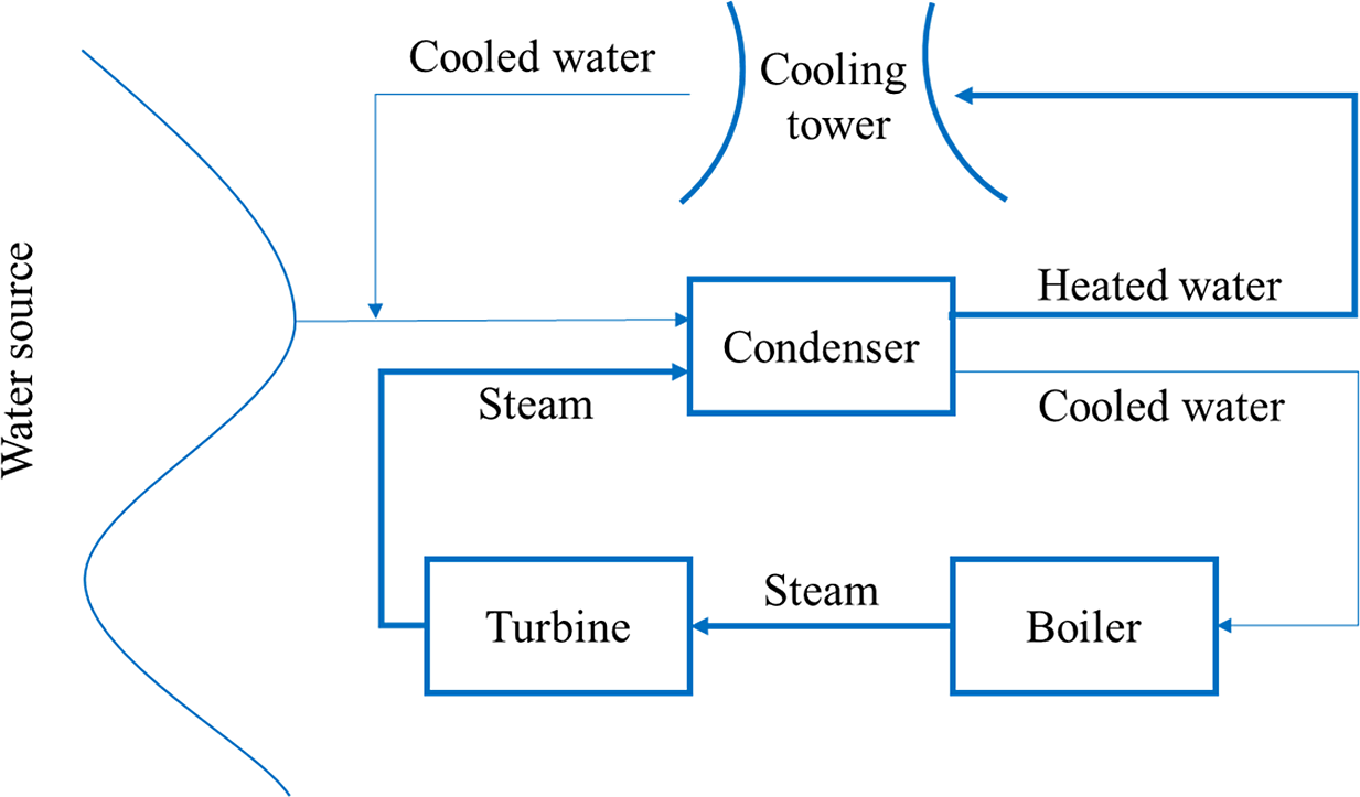
Figure 1. Recirculating cooling system with a cooling tower.
Evaporation in towers is either “natural,” happening in natural draft towers, or assisted by fans in mechanical draft towers. Natural draft towers are tall, hyperboloid-shaped towers, a structure commonly associated with nuclear power plants.Footnote 3 Often visible plumes of steam from cooling towers are visible indicators that nuclear power plants emit water into the air. The image of the hyperboloid-shaped towers often has a plume of steam rising above it.
On several occasions in the past 10 years, the National Weather Service attributed precipitation near power plants to plumes coming from cooling towers. For example, on January 23, 2013, plumes from the Beaver Valley Nuclear Power Station caused snow in an area about 24 miles downwind from the power plant.Footnote 4 Other cases include precipitation caused by a gas power plant in Dodge City, KSFootnote 5 , and by the coal and oil-fueled Miami Fort Power Station.Footnote 6
3. Literature Review
There is little research in the scientific literature on the effects of power plants on microclimates. One dated exception is a report by Huff et al. (Reference Huff, Beebe, Jones, Morgan and Senonin1971), who provide a survey of then-contemporary work on the effects of cooling towers on climate. The authors find that mechanical draft towers can cause fog and icing, events identified most often because it is easy to observe them. On the other hand, natural draft towers (being taller than mechanical draft towers) are claimed to be more likely to affect cloud formation and precipitation. The authors find that cooling tower plumes can cause cloud formation, though no “meteorologically acceptable” study assessing the possibility that these plumes “augment precipitation and cloud systems associated with naturally occurring storms” was found at the time (Huff et al., Reference Huff, Beebe, Jones, Morgan and Senonin1971). Surprisingly, no articles can be found written after the 1970s on the subject.
Similarly, little attention has been paid to the effects of power plants on local agriculture. In a recent study, Junkermann and Hacker (Reference Junkermann and Hacker2018) find that coal power stations’ emissions of ultrafine particles change global precipitation patterns. One may conjecture that such change affects crop yields but a study confirming this conjecture has yet to be completed. Burney and Ramanathan (Reference Burney and Ramanathan2014) report the effects of short-lived climate pollutants on wheat and rice yields in India. With respect to clean energy sources, Kaffine (Reference Kaffine2019) builds on recent findings from natural science literature that wind farms change local microclimate and finds evidence for a positive county-level effect of wind farms on local soybean, corn, and hay, and wheat yields. Chen (Clay et al., Reference Clay, Lewis and Severnini2019), using farm-level data from Illinois, finds a positive effect of wind farms on corn and soybean yields. Metaxoglou and Smith (Reference Metaxoglou and Smith2020) find that reduction in NOx emissions due to closures of coal power plants and installation of abatement technologies on the remaining coal power plants led to increase in corn and soybean yields.
4. Data
The data on nuclear units’ commission years and nameplate capacities were combined with data on crop yields and meteorological data for the period from 1972 to 1991.
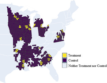
The yearly county-level crop yield data (in bushels per acre) come from the United States Department of Agriculture’s National Agricultural Statistics Service. To analyze a balanced panel, some of the counties are omitted from the final data set. The results for the unbalanced panel estimates are presented in the Online Appendix. This article focuses on soybeans and corn, two of the most important crops in the agriculture of the United States. The maps of soybeans and corn counties are presented in Figures 3–6.
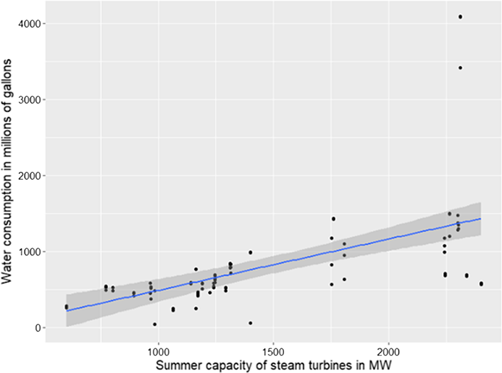
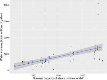
Figure 2. Water consumption in June, July, and August of 2019 across nuclear units with recirculating cooling systems. Each dot represents a particular month. Fitted line and 95% confidence interval from the simple OLS superimposed.
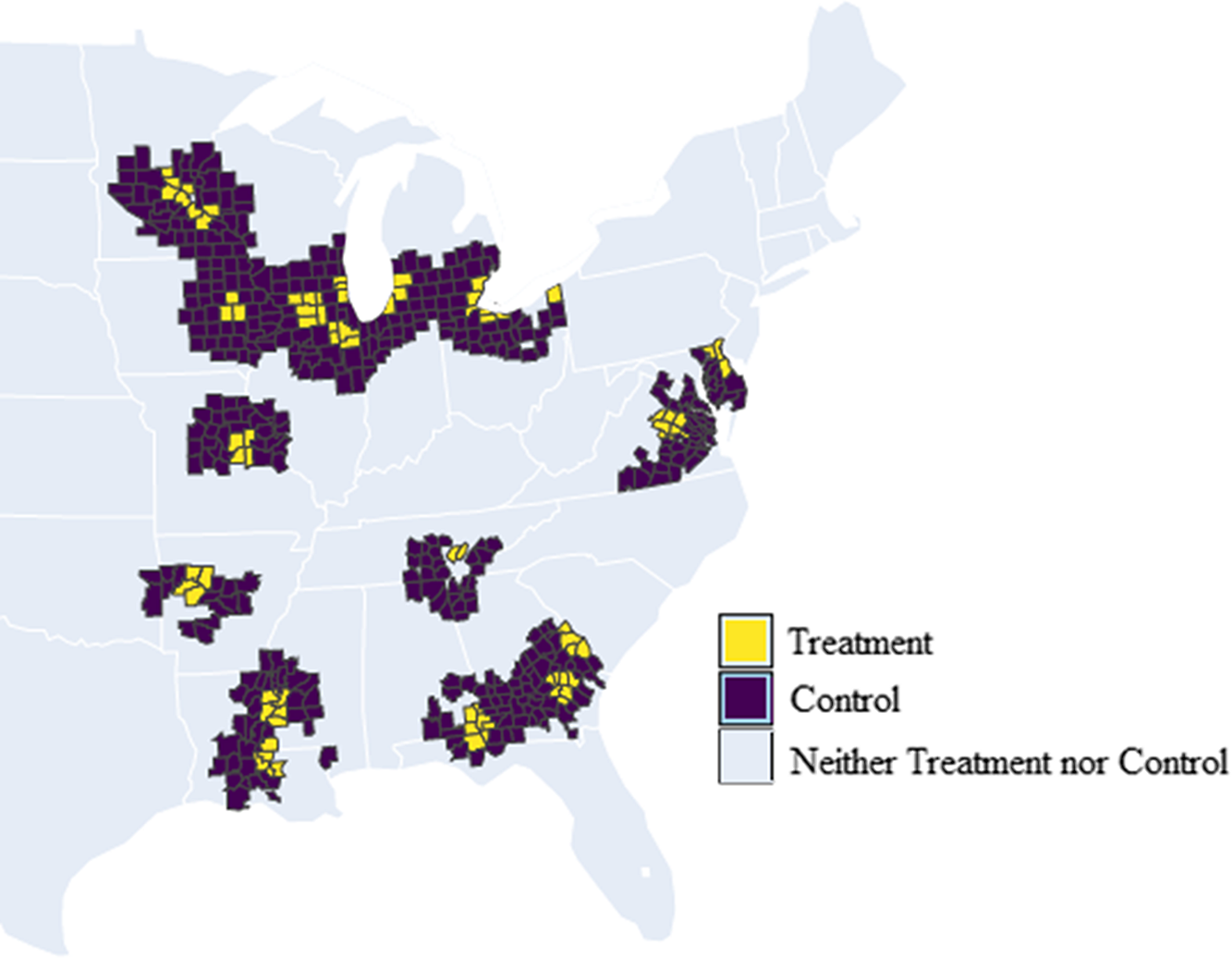
Figure 3. Soybean counties, Control 1.
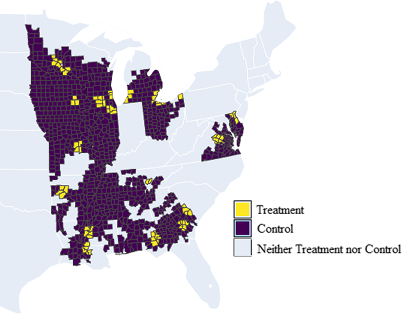
Figure 4. Soybean counties, Control 2.
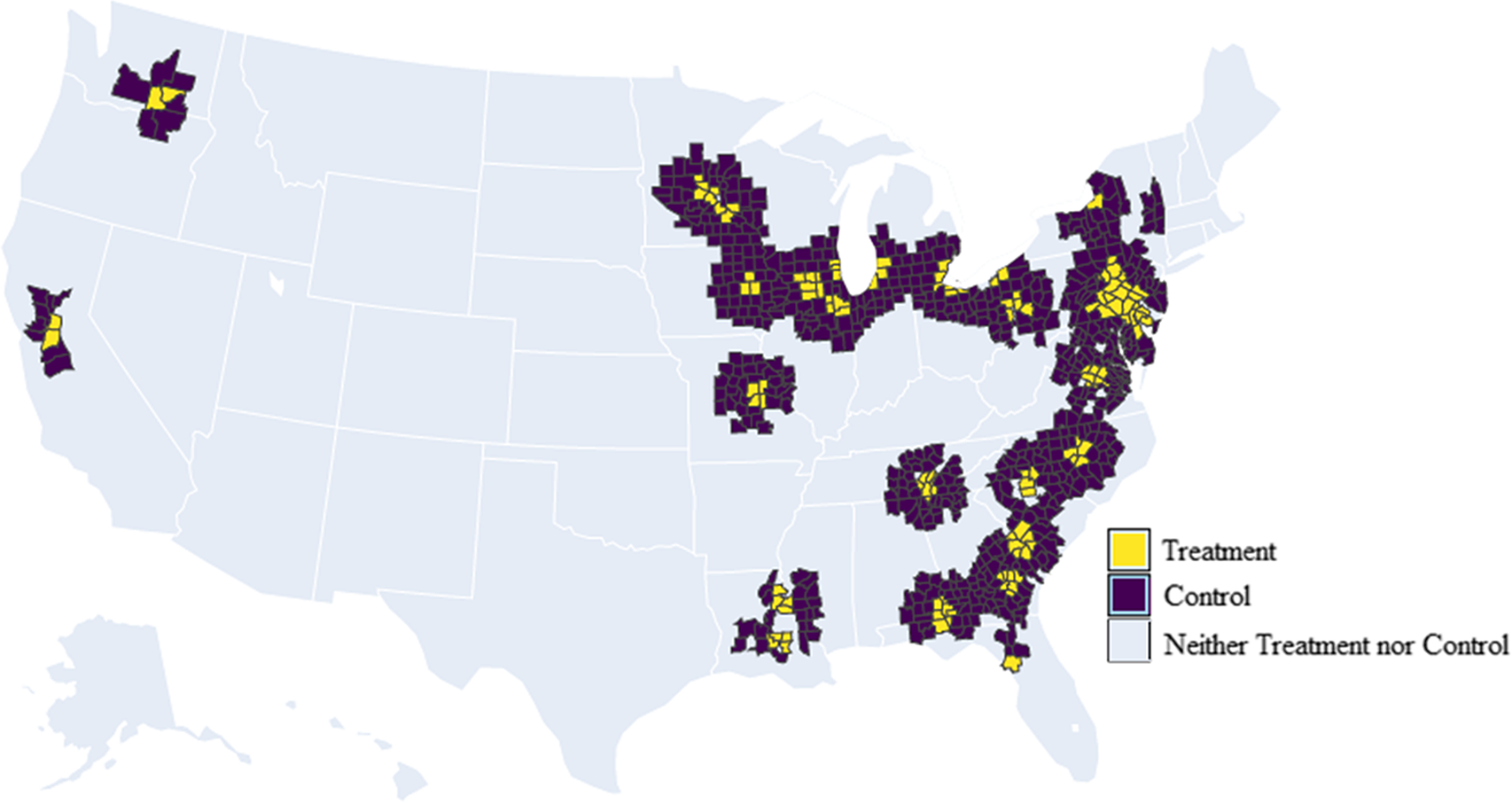
Figure 5. Corn counties, Control 1.
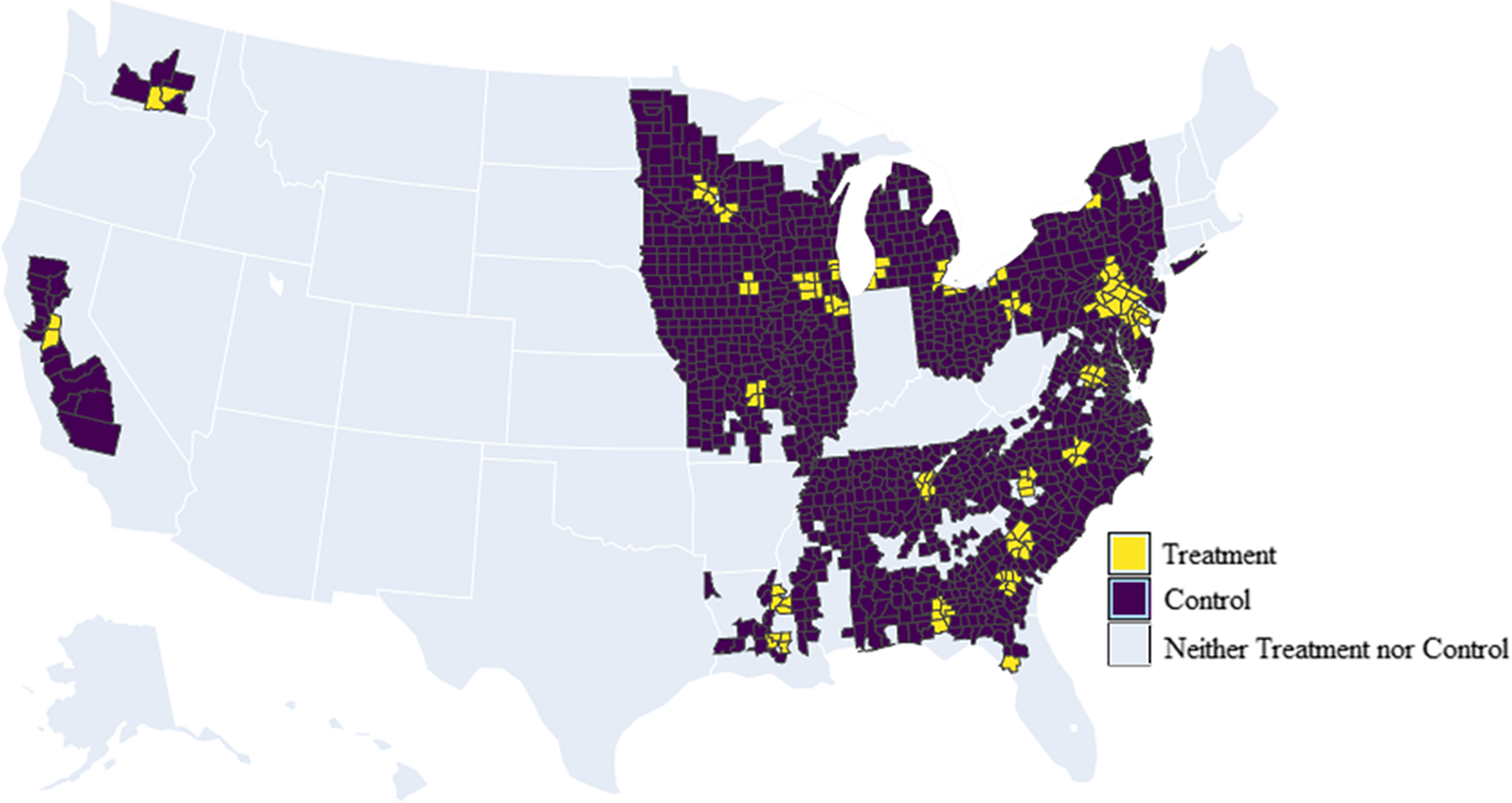
Figure 6. Corn counties, Control 2.
Common weather variables used in the literature are growing season growing degree days (GDD) and precipitation (e.g., Miao et al., Reference Miao, Khanna and Huang2016; Kaffine, Reference Kaffine2019; Metaxoglou and Smith Reference Metaxoglou and Smith2020). Because of the established non-linear relationship between the crop yields and climate conditions (e.g., Schlenker and Roberts, Reference Schlenker and Roberts2006), quadratic forms of the above weather variables are used. Weather data come from the National Oceanic and Atmospheric Administration (NOAA). The temperature data used to derive growing season (April through September) GDD values come from NOAA’s Global Historical Climatology Network data. Because these are station-level data, county-level GDDs were determined as GDDs from the station closest to the county’s centroid.Footnote 7 The period from April to September is used in, for example, Kaffine (Reference Kaffine2019). According to the USDA 1997 and 2010 reports, most states start planting soybeans in early May and corn in April. Harvesting for both soybeans and corn mostly starts in September (USDA, 1997; USDA 2010).
NOAA also provides monthly county-level precipitation data. Growing season precipitation values were derived by summing precipitation values from April through September. While humidity data would have been useful as well, many weather stations did not collect it during the 1970s. Limiting the data to years where humidity data were available for the entire growing season (or even summers only) leaves a short period after 1983, a time when development of nuclear power plants slowed down.
The data on nuclear power plants come from the Energy Information Administration’s Form EIA-860. The data include the location of a unit, the year the unit was commissioned, and the nameplate capacity of the unit. All commission years were shifted forward by 1 because some of the power plants were commissioned in the last months of the year and their construction could only affect crop yields in the following year. Because most nuclear power plants were built before the year EIA-860 was first gathered, only 2006 data were used, with missing information complemented by the data found on the International Atomic Energy Agency’s Power Reactor Information System. Only power plants with cooling towers (both natural and mechanical draft towers) were used in the final estimates. Nuclear power plants without cooling towers were used for the placebo tests. Data on water withdrawal by power plants come from the US EIA as well. These data are available for the years 2014–2019.
As Figure 7 shows, most of the nuclear units in the United States were built in the 1970s and 1980s. Earlier units were smaller in size, those built before 1970 being less than 300 mw. In comparison, units built after 1980 had a capacity of 1200 mw. The considered period is the 20 years from 1972 to 1991. 1972 was chosen as the start year because it is the earliest commission year in the data used. 1991 was chosen as the end year because it represents a reasonable balance between a longer time period (with more nuclear units built but possibly more variation in yields not caused by construction of nuclear power plants) and a shorter time period (with more counties in the balanced panel). Also, this period was chosen because it covers the years of most active nuclear power plant construction. The results for a time period consisting of an additional 20 years, 1972–2011, are presented in the Online Appendix. Summary statistics and balance tests of the data are presented in Tables 1–4. Table 3 and Table 4 indicate there were no significant differences between the treated and control counties across the yields and predictor variables.
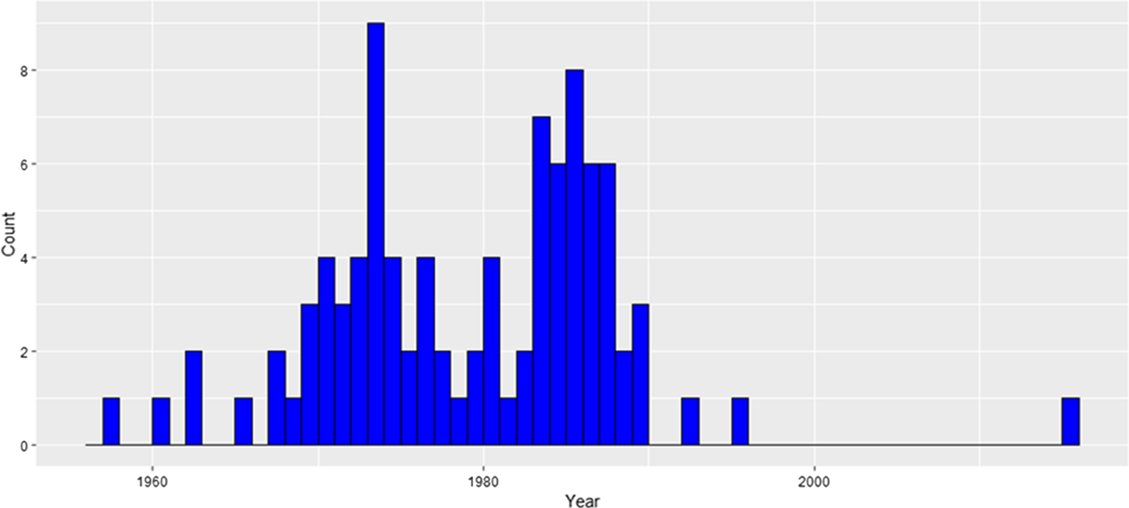
Figure 7. Nuclear units built in the United States. Most of the units were built in the 1970s and 1980s.
Table 1. Summary statistics for soybean counties
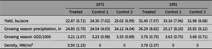
Note: “Control 1” refers to counties within 30–90 miles of distance from a nuclear power plant. “Control 2” refers to all non-treated counties in the states with nuclear power plants.
Table 2. Summary statistics for corn counties
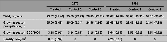
Note: “Control 1” refers to counties within 30–90 miles of distance from a nuclear power plant. “Control 2” refers to all non-treated counties in the states with nuclear power plants.
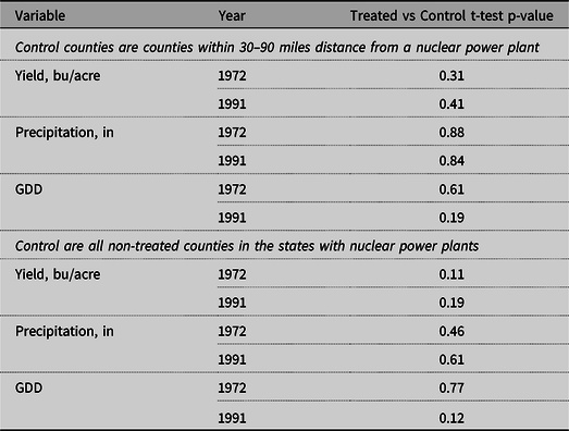
Table 3. Balance tests. Soybean counties. Treated vs Control
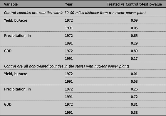
Table 4. Balance tests. Corn counties. Treated vs control
Data on economic and social characteristics of the counties come from the 1972 and 1988 County Databooks from Inter-university Consortium for Political and Social Research (ICPSR) (United States. Bureau of the Census, 1972, 1988). The data include average value of land and buildings in agriculture per acre (thousands of dollars) in 1969, percent change in farm population between 1960 and 1970, percent of the population living on the farm in 1970, percent of the labor force who are men in 1970.
5. Empirical Strategy
The yield model is estimated as follows:
 $$Yiel{d_{ct}} = \alpha + \beta \ densit{y_{ct}} + \psi {X_{{\rm{ct}}}} + Count{{\rm{y}}_c} + StateYea{{\rm{r}}_{st}} + { \in _{ct}}$$
where Yield ct is yield in county c in year t, density ct is cumulative nameplate capacity divided by the county’s area, X ct is the vector of weather variables. Equation(1) also includes county and state-year fixed effects, County c and StateYear st . Footnote 8
The effect of power plants on yields is studied through a density variable, defined as cumulative nameplate capacity in the county divided by the county’s area.Footnote 9 The same variable was used by Kaffine (Reference Kaffine2019) for wind farms and Clay et al., (2019) for coal power plants.Footnote 10 The variable of interest is aggregated within a chosen distance from the county’s centroid. The nameplate capacities of the nuclear power plants within 30 miles of the county’s centroid are summed. This distance is chosen for several reasons. First, in the absence of the exact estimates on water dispersion from cooling towers, estimates by Levy et al. (Reference Levy, Spengler, Hlinka, Sullivan and Moon2002) on particulate matter, on which Clay et al., rely, are assumed to be a close approximation. Second, cases of precipitation caused by cooling towers mentioned in the earlier “Power plants and water” section also suggest that 30 miles is a reasonable distance to choose.
While this article later shows some evidence that nuclear power plants cause higher precipitation in the counties nearby, it includes precipitation in the yield regressions. In regressions including both the density and precipitation, the density coefficient stands for the effect of nuclear power plants through more complex mechanisms (e.g., fog, icing, or limited access to sunlight due to cloud formation). As shown in the results section, this does not affect the density coefficients considerably; in all of the specifications, including precipitation decreases the size of the density coefficient, thus implying that the final estimates are conservative.
Also similar to Clay et al., control counties are chosen in one of two ways. First, control counties are defined to be those whose centroids lie within 30–90 miles from a nuclear power plant. This specification will be considered as main. Second, control counties are defined to be non-treated counties in any state where nuclear power plants were built.
In addition, a definition of control and treatment counties, taking into account wind direction, was considered. Data on wind directions from NOAA’s Integrated Surface Database were used to identify the average wind directions at the stations closest to the power plants. Counties within 30 miles of a power plant that lay downwind in a 180-degree sector were chosen as treated counties. Counties within the same distance that are not downwind of any power plant were chosen as control counties.Footnote 11
Crop yields vary by region. For example, soybean and corn yields are usually higher in the Midwestern United States (the so-called Soybean and Corn belts). Therefore, county fixed effects, η c , are added. While crop yields vary from year to year, there is a clear upward trend across all states. State-year fixed effects, λ st , are included to control for these changes in yields. Standard errors are clustered at the state level. Alternative clustering levels (county and agricultural district) are considered as well.
6. Results
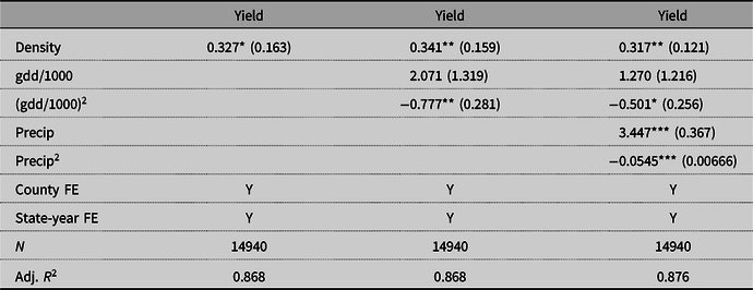
The results for soybeans are presented in Table 5. The results for corn are presented in Table 6. The observed coefficients imply that an average nuclear power plant would increase the soybean yields in nearby counties by 2% and corn yields by 1%.Footnote 12 Because density and precipitation are likely positively correlated and because density has a positive coefficient, the coefficient in column (3) is greater than in column (1) due to the positive bias of the coefficient in column (1).
Table 5. Yield regressions for soybeans
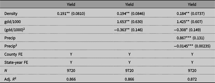
Standard errors clustered at the state level in parentheses.
* p < 0.10, **p < 0.05, ***p < 0.01.
Table 6. Yield regressions for corn
Standard errors clustered at the state level in parentheses.
* p < 0.10, **p < 0.05, ***p < 0.01.
For soybeans, regression excluding density variable and including only weather variables indicates that yields are maximized at growing season GDD of 2370 and growing season precipitation of 43.5 inches. While the average growing season GDD is greater than 2370, the average growing season precipitation is less than 43.5. This supports the argument that water steam from cooling towers may increase yields through higher precipitation.
6.1. Robustness of Results
This section discusses the results of robustness tests. The summary of the results is presented in Figure 8 and Figure 9. The graphs indicate that the results in the main specification are robust. They also indicate that the density coefficient estimate in the main specification is conservative compared to robustness check results. This implies that the estimated effect on yields may be larger than the one reported by the main specification.
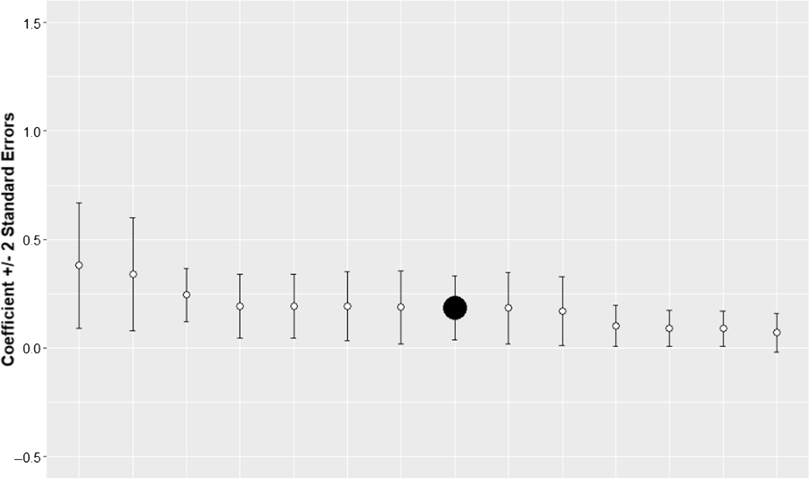
Figure 8. Coefficient estimates with standard errors for the main and robustness check specifications. Soybeans counties. The solid black point represents the main specification.
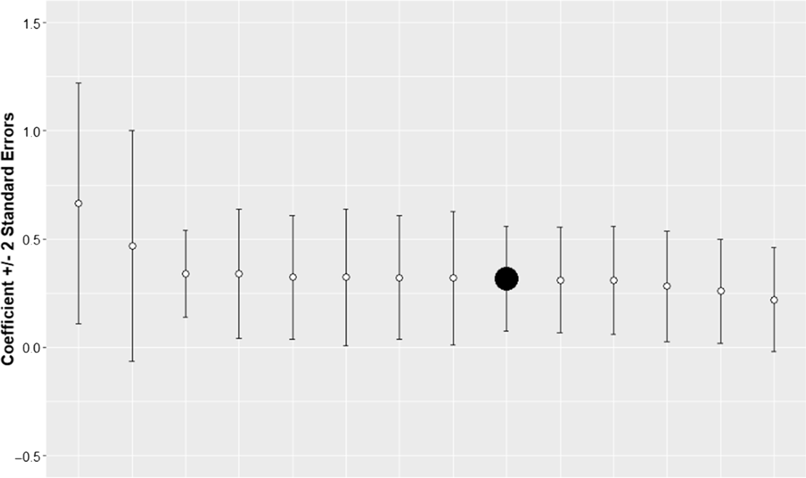
Figure 9. Coefficient estimates with standard errors for the main and robustness check specifications. Corn counties. The solid black point represents the main specification.
For brevity, detailed discussion of the robustness checks and their results are presented in the online appendix. The robustness checks considered are alternative choice of control counties, use of quadratic nuclear density variable in the regressions, regressions taking into account wind directions, use of explanatory variables binned at the quartiles (quartiles plotted in Figures 12–15), regressions with GDD calculated using a “sine” method, regressions including the number of cold days as explanatory variable, exclusion of counties with high urbanization rates (urbanization rates plotted in Figures 16 and 17), use of Palmer Drought Severity Index (Palmer, Reference Palmer1965) as explanatory variable, use of alternative clustering levels, regressions on the extended timeline (40 years between 1972 and 2011), and regressions using unbalanced panel.
6.2 Identifying Assumptions
One of the key assumptions behind the analysis above is the parallel trends in treatment and control groups in the absence of treatment. That is, it is assumed that if nuclear power plants were not constructed, yields in the treatment and control counties would be evolving in the same way. Hence, the yield data are tested for the presence of parallel pre-trends.
Roth (Reference Roth2021), identifies that a common practice in the literature for testing for pre-trends is an estimation of the following model (adapted to the notation used earlier in this paper):
 $$Yiel{d_{ct}} = \mathop \sum \limits_{l \ne 0} {\beta _l} \times {1_{ct}}(t = l) \times {D_c} + \psi {X_{ct}} + Count{{\rm{y}}_c} + StateYea{{\rm{r}}_{st}} + { \in _{ct}}$$
where
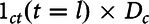 $$1_{ct}\left(t=l\right){\times}D_{c}$$
is an indicator variable for a county-level observation l years before or after the first nuclear power plant was built nearby. Thus, β
l
should be close to zero for negative l because it can be interpreted as the effect of nuclear power plant development l years before actual development. Similarly, β
l
should be significant for positive l as it can be interpreted as the effect after a nuclear power plant was built nearby. The results are presented in Figure 10 for soybeans and in Figure 11 for corn counties. Recent literature, however, suggests that the test described above may not be reliable.Footnote
13
$$1_{ct}\left(t=l\right){\times}D_{c}$$
is an indicator variable for a county-level observation l years before or after the first nuclear power plant was built nearby. Thus, β
l
should be close to zero for negative l because it can be interpreted as the effect of nuclear power plant development l years before actual development. Similarly, β
l
should be significant for positive l as it can be interpreted as the effect after a nuclear power plant was built nearby. The results are presented in Figure 10 for soybeans and in Figure 11 for corn counties. Recent literature, however, suggests that the test described above may not be reliable.Footnote
13
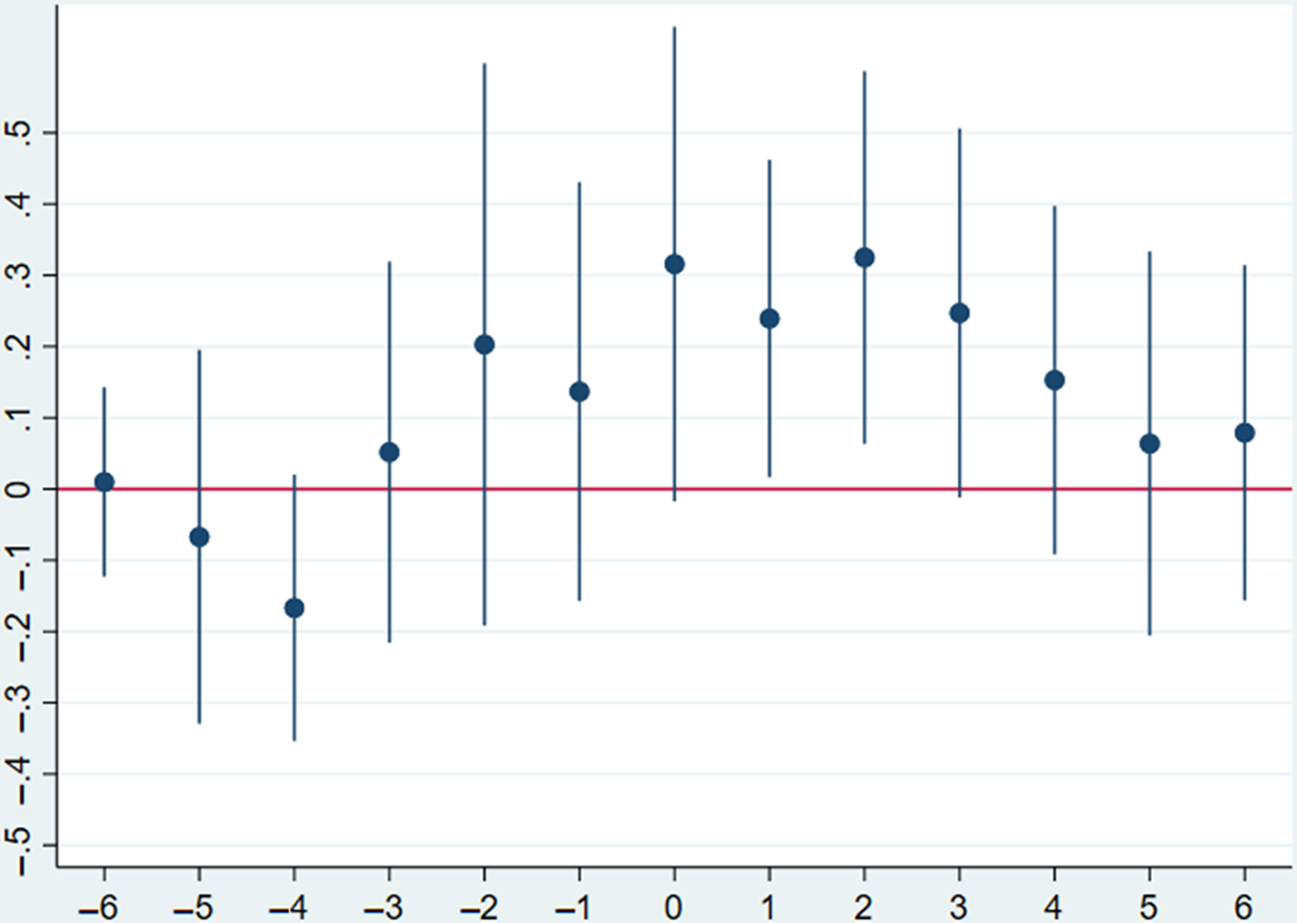
Figure 10. Log of crop yields vs the years before/after the nuclear power plant commission. Soybeans.
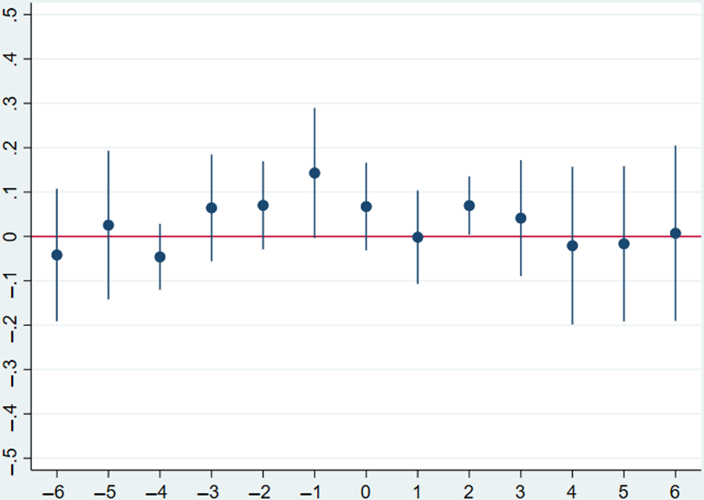
Figure 11. Log of crop yields vs the years before/after the nuclear power plant commission. Corn.
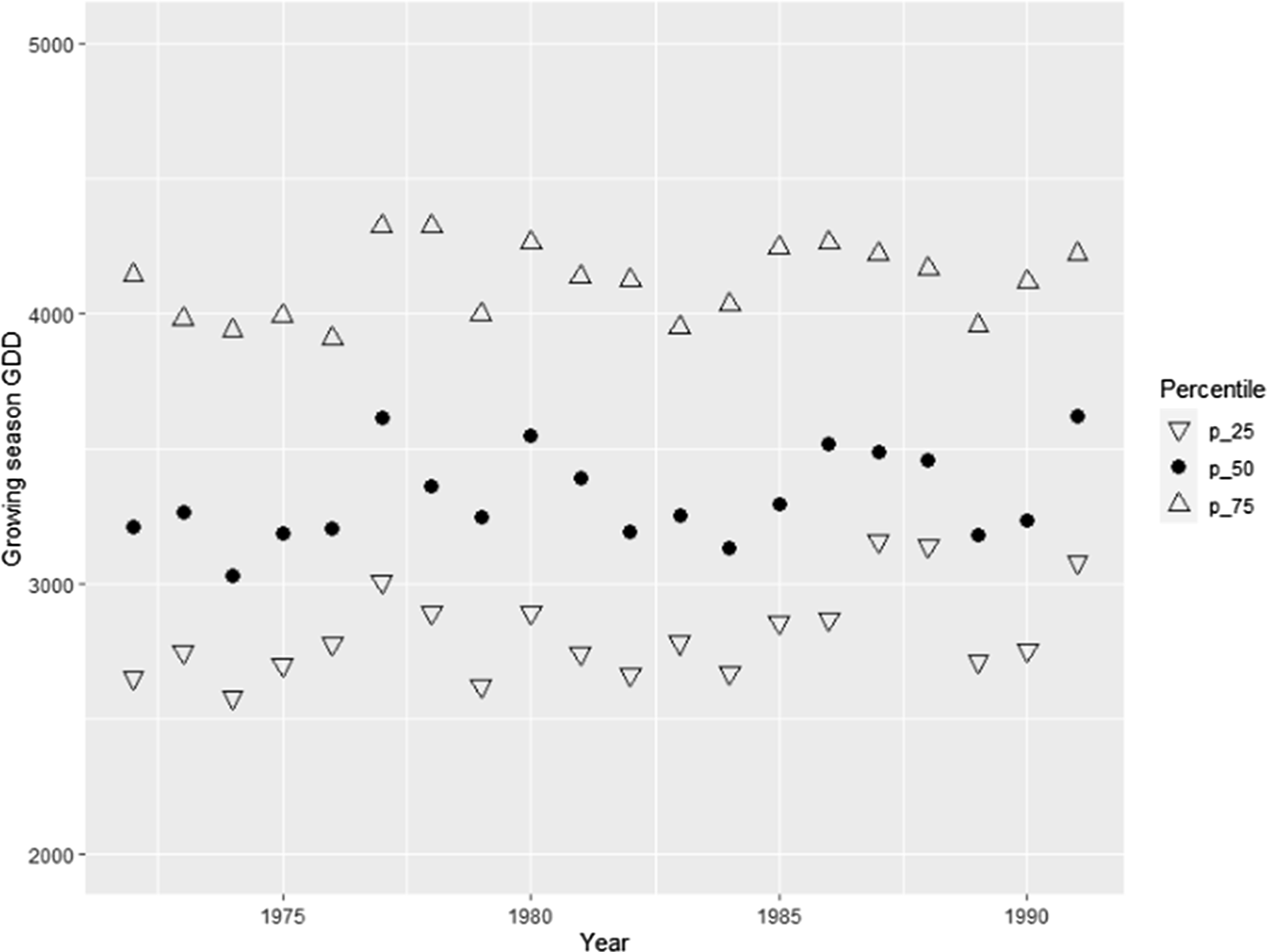
Figure 12. Quartiles of growing season GDD. Soybeans counties.
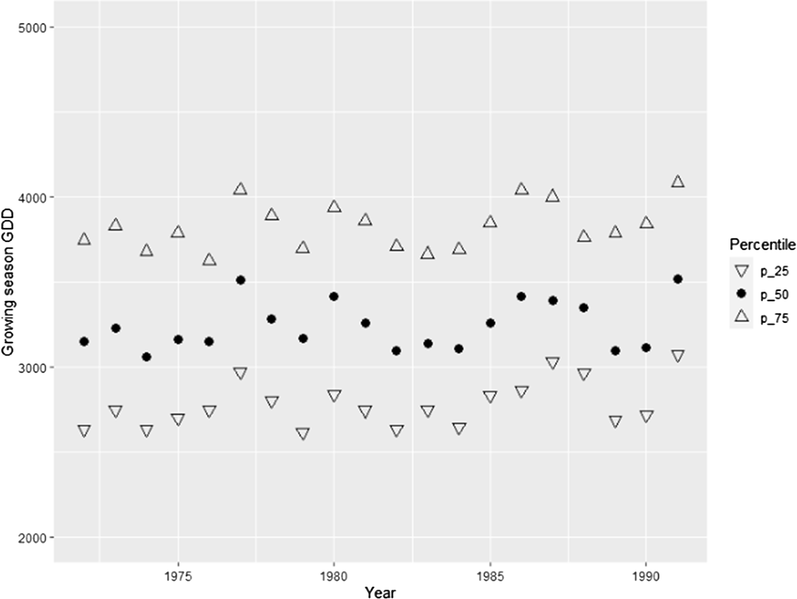
Figure 13. Quartiles of growing season GDD. Corn counties.
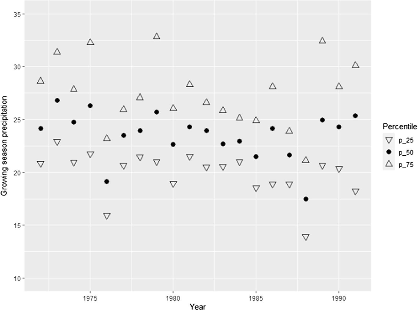
Figure 14. Quartiles of growing season precipitation. Soybeans counties.
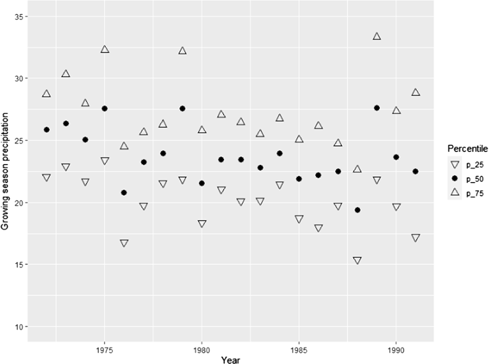
Figure 15. Quartiles of growing season precipitation. Corn counties.
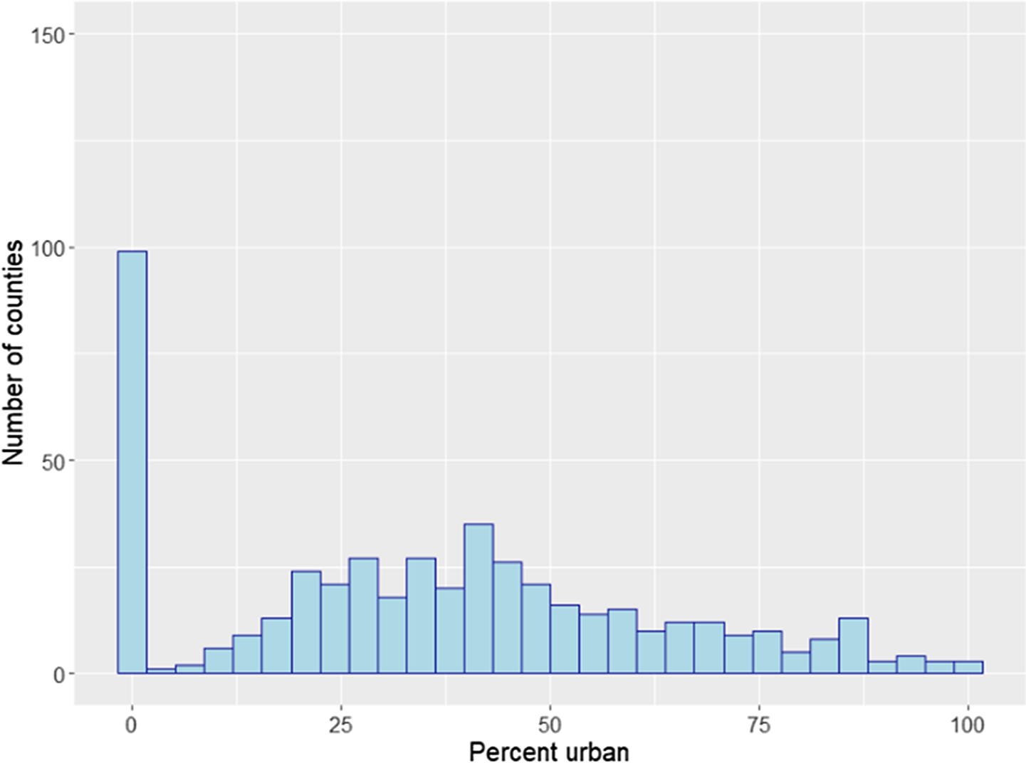
Figure 16. Distribution of counties by urbanization rate. Soybean counties.
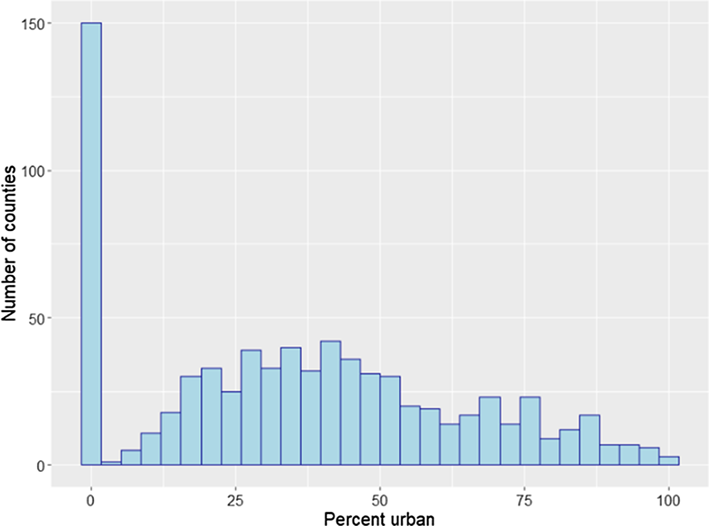
Figure 17. Distribution of counties by urbanization rate. Corn counties.
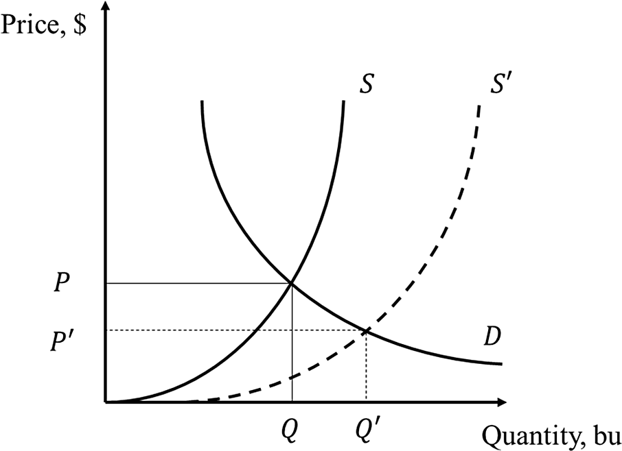
Figure 18. Effect of increase in yields.
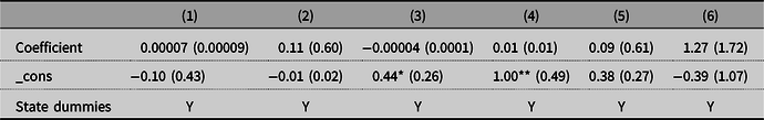
The task, then, is to present the evidence that power plant sites were not chosen based on the crop yields of the nearby counties. Simple linear models are estimated to test if the density change between 1972 and 1982 is correlated with environmental and socioeconomic factors that may have been considered in siting decisions. The factors considered are average value of land and buildings in agriculture per acre in 1969, percent change in farm population between 1960 and 1970, percent of the population living on the farm in 1970, percent of the labor force who are men in 1970, average growing season GDD between 1972 and 1974, average growing season precipitation between 1972 and 1974.Footnote 14 The results are presented in Table 7 and Table 8. Absence of statistically significant coefficients implies that nuclear power plant siting was not determined by nearby crop yields.
Table 7. Testing for common trends. Soybeans counties

Heteroscedasticity-robust standard errors in parentheses.
*p < 0.10, **p < 0.05, ***p < 0.01.
Coefficients: (1) Average growing season GDD, 1972–1974. (2) Average growing season precipitation, 1972–1974. (3) Average value of land and buildings in agriculture per acre (thousands of dollars), 1969. (4) Percent change in farm population between 1960 and 1970. (5) Percent of the population living on the farm, 1970. (6) Percent of the labor force who are men, 1970.
Table 8. Testing for common trends. Corn counties
Heteroscedasticity-robust standard errors in parentheses.
*p < 0.10, **p < 0.05, ***p < 0.01.
Coefficients: (1) Average growing season GDD, 1972–1974; (2) Average growing season precipitation, 1972–1974. (3) Average value of land and buildings in agriculture per acre (thousands of dollars), 1969. (4) Percent change in farm population between 1960 and 1970. (5) Percent of the population living on the farm, 1970. (6) Percent of the labor force who are men, 1970.
The NRC presents a list of considerations taken when choosing a site for a nuclear power plant.Footnote 15 While this list does mention factors such as meteorology and hydrology of the potential nuclear power plant site, nothing seems to suggest that the crop yields are considered as well.
6.3. Mechanism
6.3.1. Placebo Test
A placebo test considers the yield changes around power plants without cooling towers. If the observed effect is due to the cooling towers, rather than the construction of the nuclear power plants, regressions with nuclear power plants without cooling towers should not have significant coefficients on the density variable. The results for the placebo tests are presented in the Online Appendix in Table A.28. The density coefficients were not significant. Thus, the placebo test results support the proposition that the effects observed above are due to the cooling towers of the nuclear power plants.
6.3.2 Precipitation Regression
To explore the effect of nuclear power plants on local precipitation, a simple model defined as follows was estimated:
 $$\ln \, (precipitatio{{\rm{n}}_{ct}}) = \alpha + \beta \ densit{y_{ct}} + \gamma\ density_{ct}^2 + Count{{\rm{y}}_c} + StateYea{{\rm{r}}_{st}} + { \in _{ct}}$$
where the variables are defined the same way as in the main regression. The results are presented in Table 9. The main specification shows evidence for increased precipitation in spring, while the upwind-downwind specification shows evidence for increased precipitation over the entire growing season. The coefficients imply that a typical power plant would increase spring precipitation in the main specification by 3%. Assuming spring precipitation contains a third of growing season precipitation, according to Table 5, holding density constant, a 1% increase in growing season precipitation would increase soybean yields by 2.7%. Such an increase is consistent with the results in Table 5.
Table 9. Effect on microclimate
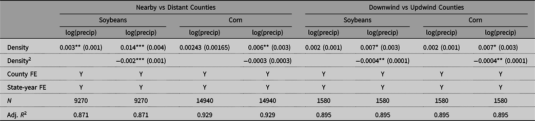
Standard errors clustered at the state level in parentheses.
* p < 0.10, **p < 0.05, ***p < 0.01.
6.3.3 Nuclear Power Plant Construction and Land Use
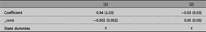
An alternative mechanism could be that a siting of a nuclear power plant deters nearby construction, thus keeping productive land for agriculture. It would be reasonable to suggest then that the placement of a nuclear power plant will affect the amount of land used in agriculture. To check this, a regression exploring the relationship between the change in acres of farmland between 1978 and 1982 and change in density between 1972 and 1977 was estimated. The results in Table 10 (Table 11 for corn) indicate no correlation between these variables and, hence, refute this alternative explanation.
Table 10. Change in density between 1978 and 1982 vs change in land used for farming. Soybeans
Heteroscedasticity-robust standard errors in parentheses.
*p < 0.10, **p < 0.05, ***p < 0.01.
Coefficients: (1) Change in acres of farmland, millions of acres, 1972–1974; (2) Percentage change in acres of farmland, millions of acres, 1972–1974.
Table 11. Change in density between 1978 and 1982 vs change in land used for farming. Corn
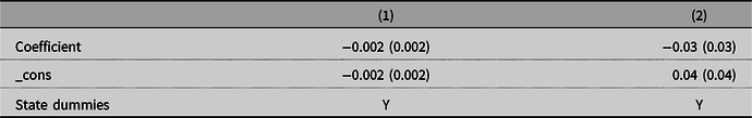
Heteroscedasticity-robust standard errors in parentheses.
*p < 0.10, **p < 0.05, ***p < 0.01.
Coefficients: (1) Change in acres of farmland, millions of acres, 1972–1974; (2) Percentage change in acres of farmland, millions of acres, 1972–1974.
7. Economic Implications
Based on the results in the previous section, welfare effect calculations of the external effects of nuclear power plants on crop yields can be performed. Metaxoglou and Smith (Reference Metaxoglou and Smith2020) point out that crops like corn and soybeans have low elasticities of supply and demand. Thus, an increase in yields and, thus, increase in quantity produced would lead to a decrease in price and would make consumers better off and farmers worse off. Following similar procedures, counterfactual quantities, prices, and welfare changes for soybeans and corn consumers and producers were calculated. The general procedure is presented in the Appendix. For comparability of the results, the demand and supply elasticities computed by Metaxoglou and Smith (Reference Metaxoglou and Smith2020) are used to calculate the welfare effects of nuclear power plants.Footnote 16 The results, presented in Table 12, suggest that consumer surplus increased annually for soybean consumers by $278 million and for corn consumers by $267 million. Producer surplus decreased annually for soybean farmers by $161 million and for corn farmers by $156 million.
Table 12. Welfare change
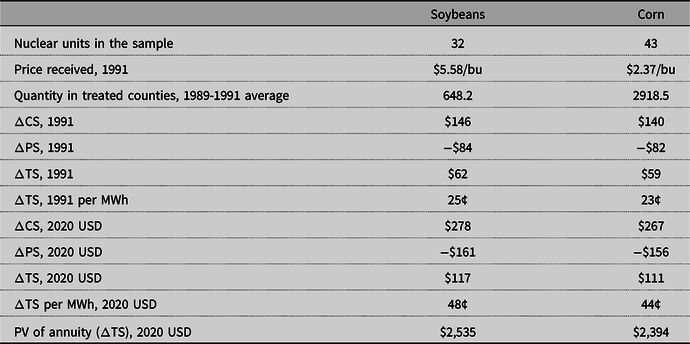
Note: Quantity is measured in millions of bushels. Changes in consumer surplus, producer surplus, total surplus, and the present value of the annuity are measured in millions.
If nuclear power plants operate for 35 years,Footnote 17 with an interest rate of 3%, the annual benefits combine into an annuity with the present value of $2.5 billion from the increase in soybean yields and $2.4 billion from the increase in corn yields.Footnote 18
These annual benefits and costs look significant when compared to the estimated construction cost of a nuclear power plant of $2–$10 billion.Footnote 19 At the assumed prices, adjusted for inflation, the total value of these two crops produced in 2019, however, is $98 billion. Thus, in the context of the entire country, this loss in producer surplus corresponds to a small fraction of the total value of crops. The results above also indicate smaller welfare effects compared to those found by Metaxoglou and Smith (Reference Metaxoglou and Smith2020), who find an increase in consumer surplus of $3.77 billion and a decrease in producer surplus by $2.17 billion for soybeans and corn combined. The yearly change in producer surplus estimates is also smaller than the estimated annual damages to crops of $1.2 billion from nitrogen oxides and volatile organic compounds pollutions estimated by Muller and Mendelsohn (Reference Muller and Mendelsohn2007).
With a 90% capacity factor for nuclear power plants, the estimates translate to benefits of 90 ¢/MWh per year from the two considered crops. While this estimate is lower than Kaffine’s (Reference Kaffine2019) result of $5.33/MWh, the total benefits are still considerable and are greater than the nuclear fuel cost of 0.06 ¢/MWh.Footnote 20
One may wonder about the opportunity cost of water used by the power plants. Most of the nuclear power plants, like most of the soybeans and corn-growing counties, are located in the eastern part of the United States, where water for irrigation is abundant. Table 13 explores the relationship between the PDSI and water withdrawal levels by nuclear power plants. The results suggest that the water withdrawal levels are not affected by droughts. Thus, water management may not be a significant issue for nuclear power plants. This agrees with the findings by Eyer and Wichman (2018). They find that water scarcity shifts electricity generation from coal to natural gas power plants and does not affect generation by nuclear power plants.
Table 13. Water withdrawal volume and withdrawal rate for nuclear power plants
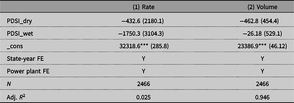
Standard errors clustered at the power plant level in parentheses.
*p < 0.10, **p < 0.05, ***p < 0.01.
The dependent variables are water withdrawal intensity rate (in gallons/MWh) and water withdrawal volume (in million gallons). PDSI_dry refers to PDSI below -3 and PDSI_wet refers to PDSI above 3. The omitted variable is PDSI between −3 and 3.
8. Conclusions
Nuclear power, despite the controversy around its safety, is still an attractive source of energy because it does not have “dirty” emissions that would have negative effects on human health or contribute to global climate change through carbon emissions. However, just like many other power plants, nuclear plants emit a significant amount of water steam into the atmosphere through their cooling systems, which can influence nearby precipitation and humidity. This article investigates the effect of nuclear power plants on nearby agriculture and find a significant positive effect on soybean and corn yields. An average nuclear power plant increases local soybean yields by 2 percent and corn yields by 1 percent. The increase in yields in the two crops translates to benefits of $229 million (2020 US dollars) per year, a combination of a $317 million loss to farmers and $546 million benefit to consumers.
Supplementary material
For supplementary material accompanying this paper visit https://doi.org/10.1017/aae.2021.32
Appendix: Calculating Welfare Changes
Given the observed price and quantity, the goal is to estimate counterfactual price and quantity, that is, the price and quantity in the absence of increased yields. See Figure 18. Suppose the demand and supply curves in the absence of an increase in yields are given by D and S, the counterfactual price and quantity are P and Q. Due to the increase in yields, however, the supply curve shifts to S’. The observed price and quantity are P’ and Q’.
With constant elasticities, demand and supply curves are given by Q = a d P η d and Q = a s P η s , where η d and η s are elasticities of demand and supply and a d and a s are constants.
 $$\Delta {\rm{CS}} = \mathop \int \limits_{{P^\prime }}^P {a_d}{P^{{\eta _d}}}dP$$
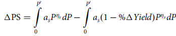 $$\Delta {\rm{PS}} = \mathop \int \limits_0^{{P^\prime }} {a_s}{P^{{\eta _s}}}dP - \mathop \int \limits_0^{{P^\prime }} {a_s}(1 - {\rm{\% }}\Delta Yield){P^{{\eta _s}}}dP$$
This can be shown to result in (see Metaxoglou and Smith Reference Metaxoglou and Smith2020, for intermediate steps):
 $$\Delta {\rm{CS}} = {{{Q^\prime }{P^\prime }} \over {1 + {\eta _d}}} * \left(\left(1 + {{{\rm{\% }}\Delta Yield} \over {{\eta _s} - {\eta _d}}}\right) - 1\right)$$
 $$\Delta {\rm{PS}} = {\rm{\% }}\Delta Yield \times {{{Q^\prime }{P^\prime }} \over {1 + {\eta _s}}} \times {\left(1 + {{{\rm{\% }}\Delta Yield} \over {{\eta _s} - {\eta _d}}}\right)^b} - {{{Q^\prime }{P^\prime }} \over {1 + {\eta _s}}} \times \left(\left(1 + {{{\rm{\% }}\Delta Yield} \over {{\eta _s} - {\eta _d}}}\right) - 1\right)$$


 Open access