


1. Introduction
Panzar and Willig (Reference Panzar and Willig1981) and Baumol, Panzar, and Willig (Reference Baumol, Panzar and Willig1982) introduced the concept of economies of scope and scale, which we use to characterize the effects of diversification and size on the costs of food production. A firm/farm has options to increase or decrease the volume of food produced (economies of scale), or it can increase or decrease the number of outputs/foods produced (economies of scope). The goal of both scale and scope adjustments is to reduce the average cost per unit produced. Scale economies arise mainly by spreading fixed costs over more production and reducing marketing costs by buying larger volumes of inputs and selling larger volumes of output. Scope economies arise from various sources, including complementarities among types of production and the spreading of labor demands to permit more gainful employment over the production year. Firms/farms need to identify and exploit economies of scale and scope to be competitive and adaptive, and hence more productive.
Livestock production dominates Norwegian agriculture in all regions. About 30% of farms are specialized in dairy farming. However, farmers in Norway face unfavorable production environments of harsh climate and extensive areas of rugged terrain. Only 3% of the total area is under agricultural cultivation, and farm production faces a long winter in most regions (October–March) and a short growing season (April–September). Thus, farmers depend heavily on growing and conserving grass during the long summer days (Steinshamn et al., Reference Steinshamn, Nesheim and Bakken2016).
In response to unfavorable conditions for farming, and with the aim to keep farm incomes at levels that enable farm families to enjoy standards of living in line with the rest of the population, successive Norwegian governments have implemented substantial support programs. Other measures, linked with these programs, have been put in place to sustain preexisting patterns of agriculture. National farm policy is developed in annual negotiations on prices and other financial support to agriculture between the government and farmers’ unions.
Mainly because production has been subsidized, Norway has some problems with food surplus, mainly of milk production. To avoid overproduction, the government imposed quotas in 1983 to limit the amount of milk farmers could sell.Footnote 1 From 1996, the government implemented a system for restricted redistribution of milk quotas using region-based regulated quota sales. Despite this easing of the rules, the ability of dairy farmers to adjust the scales of their milk production to changes in economic and technological conditions remains somewhat constrained. Moreover, there is also a law regulating the transfer of ownership of farms. With few exceptions, this law has ensured that farms stay within the same families for generations (Sipiläinen, Kumbhakar, and Lien, Reference Sipiläinen, Kumbhakar and Lien2014).
Although these policies fulfill certain political or social welfare objectives, some seem likely to limit farmers’ abilities to adjust the sizes of their farms and/or the scale or scope of their production to changes in economic and technological conditions. Rules and regulations that prevent farmers from reaching the efficient scale of operation, or from reducing average costs by diversification, will limit productivity changes and thereby the competitiveness of farming (e.g., Rasmussen, Reference Rasmussen2010). Quota regulations appear to have slowed the expansion of dairy farms, with the result that growth in output and productivity has been held back (Flaten, Reference Flaten2002; Kumbhakar et al., Reference Kumbhakar, Lien, Flaten and Tveterås2008; Løyland and Ringstad, Reference Løyland and Ringstad2001; Sipiläinen, Kumbhakar, and Lien, Reference Sipiläinen, Kumbhakar and Lien2014). In addition to direct subsides, Norwegian agriculture is protected by restrictions on imports for a range of foods. There is international pressure on the country to cut back on border protection and on output-related subsidies. Therefore, there is a need to assess whether there are now significant unexploited opportunities for farmers to reduce cost through scale and/or scope adjustments. Thus, the aim in the study is to analyze the potential cost reduction on Norwegian dairy and crop farms via economies of scale and scope. Because of the big differences in production environments for agriculture across Norway, we have also sought to address the effect of location (region) on economies of scale and scope.
Estimating economies of scale and scope has received much attention in the economics literature in different sectors. For instance, in telecommunications (Bloch, Madden, and Savage, Reference Bloch, Madden and Savage2001), education (Cohn, Rhine, and Santos, Reference Cohn, Rhine and Santos1989; Worthington and Higgs, Reference Worthington and Higgs2011), banking (Awdeh, El-Moussawi, and Nasser, Reference Awdeh, El-Moussawi and Nasser2016; Berger, Hanweck, and Humphrey, Reference Berger, Hanweck and Humphrey1987), water (Garcia, Moreaux, and Reynaud, Reference Garcia, Moreaux and Reynaud2007), health care (Given, Reference Given1996; Weaver and Deolalikar, Reference Weaver and Deolalikar2004), and utilities (Filippini and Farsi, Reference Filippini and Farsi2008). There are also a number of studies estimating economies of scale and scope in agriculture. Ray (Reference Ray1982) estimated the overall cost reduction in U.S. livestock and crop farms and reported that joint production of the two outputs would have an economic advantage. Leathers (Reference Leathers1992) found that there were economies of scale and of scope between milk and crop outputs in the state of Wisconsin (USA). Mafoua (Reference Mafoua2002) estimated the economies of scale and scope of U.S. cash grain farms and concluded that it was less expensive to produce corn, wheat, and soybeans on the same farm than on separate farms. Jin et al. (Reference Jin, Rozelle, Alston and Huang2005) investigated the economies of scale and scope for China's agricultural research system and found that strong economies of scale and small to moderate economies of scope related to the joint production of wheat and maize varieties. Lansink, Stefanou, and Kapelko (Reference Lansink, Stefanou and Kapelko2015) measured the economies of scope on Dutch crop farms over the period 1995–1999. They reported that there were economic incentives for diversification because capital is a sharable factor of production. Using a stochastic input-distance function approach, Rahman (Reference Rahman2009) revealed strong evidence of economies of scope among most crop enterprises in Bangladesh. Wimmer and Sauer (Reference Wimmer and Sauer2016) studied Bavarian dairy farms over the years 2006–2014 and reported economies of scale of 1.55 and average cost savings of 77% when milk, crop, and livestock were jointly produced. Using a homothetic production function, Løyland and Ringstad (Reference Løyland and Ringstad2001) found that, during the period 1972–1996, there was potential for cost reductions by exploiting scale economies and structural changes in Norwegian dairy farming. Fleming and Lien (Reference Fleming and Lien2009) analyzed the scope and scale economies on farms in Norway over the period 1993–2006 and concluded that considerable synergies existed between most pairs of activities.
A widely used approach to the analysis of scale and scope in previous studies of agriculture has been to use a quadratic or a translog cost function and to estimate the functions for each farm type jointly. Estimating a cost function for multiproduct farms has the drawback that a common technology across all farm types is assumed—that is, a strong assumption that the underlying technology is the same for all sample observations, regardless of differences in operating circumstances and working environments. However, farms in different regions are likely to face different production environments and opportunities, and technology sets may differ because of differences in resource endowments. For instance, in farming, there will often be differences in soil quality, the intensity of sunlight, temperature, and rainfall from place to place. The technical knowledge, capital endowments, and input composition of crop-producing farmers are likely to differ from those of dairy-producing farms. Because policy intervention and management advice may need to be different for different farm types, the difference in technology for different farm types needs to be accounted for. Moreover, if specialized farms use technology different from that used by diversified farms, yet a common technology is assumed, the results are likely to be biased. For instance, according to Triebs et al. (Reference Triebs, Saal, Arocena and Kumbhakar2016), results suggesting the presence of economies of scope may actually be a result of scale economies. If the technology is different between the farm types, separate cost functions may be needed. In this study, we allowed farm-type technologies to be different and tested whether such an assumption is supported by the data. We implemented this approach using a “flexible technology” technique, introduced by Triebs et al., in which all the technologies are combined into a single equation using dummy variables for type of firm. Another advantage of this method is that it avoids the problem of zero data values in a translog function.Footnote 2 There is evidence that replacing zero values by some arbitrary small positive number can influence the results (Pulley and Humphrey, Reference Pulley and Humphrey1993).
The flexible technology approach accounts for technology heterogeneity, and, unlike Triebs et al. (Reference Triebs, Saal, Arocena and Kumbhakar2016), we have also accounted for regional differences. Thus, this study appears to be the first use of the flexible technology approach to the assessment of economies of scale and scope of the agricultural sector, accounting for heterogeneity. Moreover, we had the advantage of a large panel database at the farm level, which provided detailed information about the Norwegian farms.
The rest of the article is organized as follows: In Section 2, we address theoretical approaches to measuring scale and scope, while in Section 3 we discuss model specification. Section 4 includes a discussion of the data and definitions of the variables used in the cost function. Section 5 discusses the estimation procedure and the results, and Section 6 concludes the article.
2. Conceptual Framework
2.1. Cost Function
This section builds on approaches proposed by Baumol, Panzar, and Willig (Reference Baumol, Panzar and Willig1982) and Triebs et al. (Reference Triebs, Saal, Arocena and Kumbhakar2016). Our model includes two outputs (dairy and crop) and three farm types: mixed farms (M), which produced both crop and dairy outputs; dairy farms (D), specialized in the dairy sector; and crop farms (P), specialized in crop production.
Let Ψ = {M, D, P} be the set of farm types. Mixed farms produce the entire output vector y = (yP and yD), while dairy (D) and crop farms (P) are specialized and produce output vectors yD and yP, respectively. We allow different farm types to have different underling production possibilities. Cost functions for different farm types are defined as
 $$\begin{equation}
C = \left\{ {\begin{array}{@{}*{1}{c}@{}} \ {\begin{array}{@{}*{1}{c}@{}} {{c^m}\left( {y,w} \right)}\\ {{c^d}\left( {{y_D},{w_D}} \right)}\\ {{c^p}\left( {{y_P},{w_P}} \right)} \ \end{array}} \end{array}} \right.,
\end{equation}$$
$$\begin{equation}
C = \left\{ {\begin{array}{@{}*{1}{c}@{}} \ {\begin{array}{@{}*{1}{c}@{}} {{c^m}\left( {y,w} \right)}\\ {{c^d}\left( {{y_D},{w_D}} \right)}\\ {{c^p}\left( {{y_P},{w_P}} \right)} \ \end{array}} \end{array}} \right.,
\end{equation}$$
where C, w, y are total cost and the vectors of input prices and outputs, respectively. Equation (1) allows the cost function to be flexible across farms by allowing technologies to differ across farm types—that is, cm(y, w), cd(yD, wD), and cp(yP, wP) are the cost functions for mixed, dairy, and crop farms, respectively, and these are different as indicated by the different superscripts. The technologies in equation (1) can be written in a single equation with the use of dummy variables as follows:
 $$\begin{eqnarray}
C\left( {y,w{\rm{\ }}} \right) & = & mdum \times {c^m}\left( {y,w,\,{\tau _m}} \right) + ddum \times {c^d}\left( {{y_D},{w_D},\,{\tau _d}} \right) \nonumber\\
&& +\, pdum \times {c^p}({y_P},{w_P},{\tau _p}) + Regional\,dummies,
\end{eqnarray}$$
$$\begin{eqnarray}
C\left( {y,w{\rm{\ }}} \right) & = & mdum \times {c^m}\left( {y,w,\,{\tau _m}} \right) + ddum \times {c^d}\left( {{y_D},{w_D},\,{\tau _d}} \right) \nonumber\\
&& +\, pdum \times {c^p}({y_P},{w_P},{\tau _p}) + Regional\,dummies,
\end{eqnarray}$$
where w, y, τ are the vectors of input prices, output, and farm specific unknown technology parameters, respectively. The variables mdum, ddum, and pdum are dummy variables that take 1 if the farm is a mixed, dairy, or crop farm, respectively, or 0 otherwise. We also included five regional dummy variables for five regionsFootnote 3 (R) of Norway to assess locational differences. We dropped northern region dummy variables during estimation. We chose a translog specification for models 1 to 3 because of its flexibility (Christensen, Jorgenson, and Lau, Reference Christensen, Jorgenson and Lau1973).
Because the parameters in the previous three cost functions are different, the specification in equation (2) is mathematically equivalent to three separate equations, one for each farm type.
Equation (2) can be estimated in three different ways. The most straightforward way is to estimate a separate regression for each farm type and estimate the economies of scale and scope following the procedure of Färe (Reference Färe1986) (see, e.g., Garcia, Moreaux, and Reynaud, Reference Garcia, Moreaux and Reynaud2007). The separate estimation means the creation of subsamples with the subsequent problem of reduced degrees of freedom. Moreover, a separate regression approach implies the existence of different technologies without allowing for the possibility of testing whether this assumption is valid or not. The other possibility is to estimate a single translog or quadratic model for all farm types assuming a common technology for all farm types. As explained in the introduction, the failure to take into account the presence of heterogeneous technologies can lead to biased results. For comparison purposes, we first estimated the cost function under the assumption that all farms in a given farm type used the same technology (model 1). Then we estimated cost functions separately assuming that dairy, crop, and mixed farms used different technologies (model 2). Finally, we estimate all three cost functions in a single equation using three dummy variables (model 3), specified in equation (2). Model 3 allowed us to estimate all the technology parameters and test the hypothesis for a common technology.
2.2. Scale Economies
Equation (2) can be fitted to a quadratic or a translog function (among other function forms), either of which can be estimated using ordinary least squares/generalized least squares. Economies of scale can be calculated from the inverse of the cost output elasticity of output (Christensen and Greene, Reference Christensen and Greene1976). For multiple-output (mixed) farms, the economies of scale are the inverse of the sum of all partial cost elasticities (Panzar and Willig, Reference Panzar and Willig1977).
 $$\begin{equation}
{\rm{Economies}}\,{\rm{of}}\,{\rm{scale}}\,{\rm{for}}\,{\rm{specialized}}\,{\rm{dairy}}\,{\rm{farms}}\,{\rm{(}}Sc{y_d}{\rm{) = }}{\left[ {{\rm{\ }}\frac{{\partial {\rm{ln}}{c^d}\left( {{y_D},w,\ {\tau _d}} \right)}}{{\partial {\rm{ln}}{y_D}}}} \right]^{ - 1}}
\end{equation}$$
$$\begin{equation}
{\rm{Economies}}\,{\rm{of}}\,{\rm{scale}}\,{\rm{for}}\,{\rm{specialized}}\,{\rm{dairy}}\,{\rm{farms}}\,{\rm{(}}Sc{y_d}{\rm{) = }}{\left[ {{\rm{\ }}\frac{{\partial {\rm{ln}}{c^d}\left( {{y_D},w,\ {\tau _d}} \right)}}{{\partial {\rm{ln}}{y_D}}}} \right]^{ - 1}}
\end{equation}$$
 $$\begin{equation}
{\rm{Economies}}\,{\rm{of}}\,{\rm{scale}}\,{\rm{for}}\,{\rm{specialized}}\,{\rm{crop}}\,{\rm{farms}}\,(Sc{y_p}) = {\left[ {{\rm{\ }}\frac{{\partial {\rm{ln}}{c^p}\left( {{y_P},w,\ {\tau _p}} \right)}}{{\partial {\rm{ln}}{y_P}}}} \right]^{ - 1}}
\end{equation}$$
$$\begin{equation}
{\rm{Economies}}\,{\rm{of}}\,{\rm{scale}}\,{\rm{for}}\,{\rm{specialized}}\,{\rm{crop}}\,{\rm{farms}}\,(Sc{y_p}) = {\left[ {{\rm{\ }}\frac{{\partial {\rm{ln}}{c^p}\left( {{y_P},w,\ {\tau _p}} \right)}}{{\partial {\rm{ln}}{y_P}}}} \right]^{ - 1}}
\end{equation}$$
 $$\begin{eqnarray}
&& {\rm{Economies}}\,{\rm{of}}\,{\rm{scale}}\,{\rm{for}}\,{\rm{mixed}}\,{\rm{farms}}\,(Sc{y_m}) \nonumber\\
&&\quad = {\left[ {{\rm{\ }}\frac{{\partial {\rm{ln}}{c^m}\left( {{y_D},w,\ {\tau _m}} \right)}}{{\partial {\rm{ln}}{y_D}}} + \frac{{\partial {\rm{ln}}{c^m}\left( {{y_P},w,\ {\tau _m}} \right)}}{{\partial {\rm{ln}}{y_P}}}} \right]^{ - 1}}
\end{eqnarray}$$
$$\begin{eqnarray}
&& {\rm{Economies}}\,{\rm{of}}\,{\rm{scale}}\,{\rm{for}}\,{\rm{mixed}}\,{\rm{farms}}\,(Sc{y_m}) \nonumber\\
&&\quad = {\left[ {{\rm{\ }}\frac{{\partial {\rm{ln}}{c^m}\left( {{y_D},w,\ {\tau _m}} \right)}}{{\partial {\rm{ln}}{y_D}}} + \frac{{\partial {\rm{ln}}{c^m}\left( {{y_P},w,\ {\tau _m}} \right)}}{{\partial {\rm{ln}}{y_P}}}} \right]^{ - 1}}
\end{eqnarray}$$
Equations (3–5) show how to calculate economies of scale for three farm types in model 2 and model 3. However, a drawback of the conventional common technology approach (model 1) is that it is not feasible to estimate the economies of scale for single output farms (Triebs et al., Reference Triebs, Saal, Arocena and Kumbhakar2016). In such a case, one could estimate product-specific economies of scale (declining average incremental costs) by converting the two-output cost function estimated using model 1 into proportionate changes in cost relative to a single output. Following Baumol, Panzar, and Willig's (1982) approach, product-specific economies of scale are calculated as follows:
 $$\begin{eqnarray}
&& {\hbox{Product{-}specific}}\,{\rm{economies}}\,{\rm{of}}\,{\rm{scale}}\,Sc\left( {{y_i}} \right) \nonumber\\
&& \quad = \frac{{AI{C_i}\left( {y,w} \right)}}{{\frac{{\partial C\left( {y,w} \right)}}{{\partial {y_i}}}}} = \frac{{AIC\ ({y_i})}}{{MC\ ({y_i})}}\,{\rm{for}}\,\,\,i = D,\,P,
\end{eqnarray}$$
$$\begin{eqnarray}
&& {\hbox{Product{-}specific}}\,{\rm{economies}}\,{\rm{of}}\,{\rm{scale}}\,Sc\left( {{y_i}} \right) \nonumber\\
&& \quad = \frac{{AI{C_i}\left( {y,w} \right)}}{{\frac{{\partial C\left( {y,w} \right)}}{{\partial {y_i}}}}} = \frac{{AIC\ ({y_i})}}{{MC\ ({y_i})}}\,{\rm{for}}\,\,\,i = D,\,P,
\end{eqnarray}$$
where  $MC\ ({y_i}) = \ \frac{{\partial C( {y,w} )}}{{\partial {y_i}}}$ is the marginal cost of producing yi units of output; AIC (yi) is average incremental cost for producing output yi, that is, $AIC\ ({y_i}) = \frac{{C( {y,w} ) - C( {{y_{N - i}},w} )}}{{{y_i}}}$ for i = D, P, C(y, w) is the total cost of producing the two outputs and C(y N − i, w) is the total cost of producing the units of the ith output, and y N − i is an output vector obtained by fixing all products except product yi.
Increasing, decreasing, or constant economies of scale exists when estimated economies of scale in equations (3–5) and (6) are greater than 1, less than 1, or equal to 1, respectively.
2.3. Scope Economies
Scope economies show the benefit that arises from the joint production of the crop and dairy outputs using multiproduct technologies. The scope economy can be measured as the difference between the cost of producing both outputs on one farm and the cost of producing the same outputs on two specialized farms (Baumol, Panzar, and Willig, Reference Baumol, Panzar and Willig1982; Panzar and Willig, Reference Panzar and Willig1981); that is:
 $$\begin{equation}
{\rm{Economies}}\,{\rm{of}}\,{\rm{scope}}\, = \frac{{{c^d}\left( {{y_D},w,\ {\tau _d}} \right)\ + \ {c^p}\left( {{y_P},w,\ {\tau _p}} \right) - {c^m}\left( {y,w,\ {\tau _m}} \right)}}{{{c^m}\left( {y,w,\ {\tau _m}} \right)}}.
\end{equation}$$
$$\begin{equation}
{\rm{Economies}}\,{\rm{of}}\,{\rm{scope}}\, = \frac{{{c^d}\left( {{y_D},w,\ {\tau _d}} \right)\ + \ {c^p}\left( {{y_P},w,\ {\tau _p}} \right) - {c^m}\left( {y,w,\ {\tau _m}} \right)}}{{{c^m}\left( {y,w,\ {\tau _m}} \right)}}.
\end{equation}$$
If joint production is less expensive than separate dairy and crop production, scope economies exist. If economies of scope are greater than zero, cost savings can be achieved from mixed farming (diversification of output). If economies of scope are less than zero, it is cheaper to produce dairy and crop outputs on separate farms.
3. Model Specification
In this section, we describe the specifications of models 1, 2, and 3 and the estimation method. We used unbalanced panel data and then included the subscripts i and t, where i denotes farm with i = 1,. . ., n and time t with t = 1, . . ., t.
3.1. Model 1
We first estimated a single translog cost function, assuming a common technology for all farm types by pooling all the observations. With a translog cost function, model 1 is specified as follows:
 $$\begin{eqnarray}
{\rm{ln}}{c_{it}} & = & {\alpha _0} + {\beta _1}{\rm{ln}}{y_{Dit}} + {\beta _2}{\rm{ln}}{y_{Pit}} + \mathop \sum \limits_{j = 2}^k {\gamma _j}{\rm{ln}}{w_{jit}} + {\delta _t}t + \mathop \sum \limits_{j = 2}^J {\alpha _{jt}}{\rm{t\ ln}}{w_{jit}} \nonumber\\
&& +\, \mathop \sum \limits_{k = 1}^K {\beta _{kt}}{\rm{t\ ln}}{y_{kit}} + \mathop \sum \limits_{j = 1}^m {\theta _{1j}}{\rm{ln}}{y_{Dit}}{\rm{ln}}{w_{jit}} + \mathop \sum \limits_{j = 1}^m {\theta _{2j}}{\rm{ln}}{y_{Pit}}{\rm{ln}}{w_{jit}} \nonumber\\
&& +\, {\rho _{12}}{\rm{ln}}{y_{Dit}}{\rm{ln}}{y_{Pit}} + \frac{1}{2}\Bigg[ {\rho _1}{\rm{ln}}{y_{Dit}}{\rm{ln}}{y_{Dit}} + {\rho _2}{\rm{ln}}{y_{Pit}}{\rm{ln}}{y_{Pit}} \nonumber\\
&&+ \mathop \sum \limits_{j = 2}^k \mathop \sum \limits_{l = 2}^k {\delta _{lj}}{\rm{ln}}{w_{lit}}{\rm{ln}}{w_{jit}} + {\delta _{tt}}{t^2} \Bigg] + \mathop \sum \limits_{r = 1}^R {\varphi _r}{R_r} + {v_{it}},
\end{eqnarray}$$
$$\begin{eqnarray}
{\rm{ln}}{c_{it}} & = & {\alpha _0} + {\beta _1}{\rm{ln}}{y_{Dit}} + {\beta _2}{\rm{ln}}{y_{Pit}} + \mathop \sum \limits_{j = 2}^k {\gamma _j}{\rm{ln}}{w_{jit}} + {\delta _t}t + \mathop \sum \limits_{j = 2}^J {\alpha _{jt}}{\rm{t\ ln}}{w_{jit}} \nonumber\\
&& +\, \mathop \sum \limits_{k = 1}^K {\beta _{kt}}{\rm{t\ ln}}{y_{kit}} + \mathop \sum \limits_{j = 1}^m {\theta _{1j}}{\rm{ln}}{y_{Dit}}{\rm{ln}}{w_{jit}} + \mathop \sum \limits_{j = 1}^m {\theta _{2j}}{\rm{ln}}{y_{Pit}}{\rm{ln}}{w_{jit}} \nonumber\\
&& +\, {\rho _{12}}{\rm{ln}}{y_{Dit}}{\rm{ln}}{y_{Pit}} + \frac{1}{2}\Bigg[ {\rho _1}{\rm{ln}}{y_{Dit}}{\rm{ln}}{y_{Dit}} + {\rho _2}{\rm{ln}}{y_{Pit}}{\rm{ln}}{y_{Pit}} \nonumber\\
&&+ \mathop \sum \limits_{j = 2}^k \mathop \sum \limits_{l = 2}^k {\delta _{lj}}{\rm{ln}}{w_{lit}}{\rm{ln}}{w_{jit}} + {\delta _{tt}}{t^2} \Bigg] + \mathop \sum \limits_{r = 1}^R {\varphi _r}{R_r} + {v_{it}},
\end{eqnarray}$$
where c is total cost incurred by the farm i in year t; wj represents the price of inputs j; yDit is the quantity of dairy output by the farm i in year t; and yPit is the quantity of crop output produced by the farm i in year t. Subscripts m and k are the number of outputs and inputs used in each farm type, respectively. Note that we used the standard practice and treat outputs being measured ex post, although the production decisions that are being modeled might be based on ex ante expectations of these outputs, perhaps giving biased results, depending on how the ex ante and ex post outcomes are related (see LaFrance and Pope, Reference LaFrance and Pope2010; Tack et al., Reference Tack, Pope, LaFrance and Cavazos2015). We included regional dummy variables Rr for the five regions of Norway. All Greek letters are parameters to be estimated. The annual trend variable, t, is included to capture technical change, starting with 1 for 1991.
3.2. Model 2
The translog functions for each type of technology from equation (2) are as follows:
Mixed farms
 $$\begin{eqnarray}
{\rm{ln}}{c_{mit}} &=& \alpha _0^m + \beta _1^m{\rm{ln}}{y_{Dit}} + \beta _2^m{\rm{ln}}{y_{Pit}} + \mathop \sum \limits_{j = 2}^k \gamma _j^m{\rm{ln}}{w_{jit}} + \delta _t^mt + \mathop \sum \limits_{j = 2}^J {\alpha _{jt}}{\rm{t\ ln}}{w_{jit}} \nonumber \\
&& +\, \mathop \sum \limits_{k = 1}^K {\beta _{kt}}{\rm{t\ ln}}{y_{kit}} + \mathop \sum \limits_{j = 1}^m \theta _{1j}^m{\rm{ln}}{y_{Dit}}{\rm{ln}}{w_{jit}} + \mathop \sum \limits_{j = 1}^m \theta _{2j}^m{\rm{ln}}{y_{Pit}}{\rm{ln}}{w_{jit}} \nonumber\\
&& +\, \rho _{12}^m{\rm{ln}}{y_{Dit}}{\rm{ln}}{y_{Pit}} + \frac{1}{2}\Bigg[ \rho _1^m{\rm{ln}}{y_{Dit}}{\rm{ln}}{y_{Dit}} + \rho _2^m{\rm{ln}}{y_{Pit}}{\rm{ln}}{y_{Pit}} \nonumber\\
&& +\, \mathop \sum \limits_{j = 2}^k \mathop \sum \limits_{l = 2}^k \delta _{lj}^m{\rm{ln}}{w_{lit}}{\rm{ln}}{w_{jit}} + \delta _{tt}^m{t^2} \Bigg] + \mathop \sum \limits_{r = 1}^R {\gamma _r}{R_r} + {v_{it}}
\end{eqnarray}$$
$$\begin{eqnarray}
{\rm{ln}}{c_{mit}} &=& \alpha _0^m + \beta _1^m{\rm{ln}}{y_{Dit}} + \beta _2^m{\rm{ln}}{y_{Pit}} + \mathop \sum \limits_{j = 2}^k \gamma _j^m{\rm{ln}}{w_{jit}} + \delta _t^mt + \mathop \sum \limits_{j = 2}^J {\alpha _{jt}}{\rm{t\ ln}}{w_{jit}} \nonumber \\
&& +\, \mathop \sum \limits_{k = 1}^K {\beta _{kt}}{\rm{t\ ln}}{y_{kit}} + \mathop \sum \limits_{j = 1}^m \theta _{1j}^m{\rm{ln}}{y_{Dit}}{\rm{ln}}{w_{jit}} + \mathop \sum \limits_{j = 1}^m \theta _{2j}^m{\rm{ln}}{y_{Pit}}{\rm{ln}}{w_{jit}} \nonumber\\
&& +\, \rho _{12}^m{\rm{ln}}{y_{Dit}}{\rm{ln}}{y_{Pit}} + \frac{1}{2}\Bigg[ \rho _1^m{\rm{ln}}{y_{Dit}}{\rm{ln}}{y_{Dit}} + \rho _2^m{\rm{ln}}{y_{Pit}}{\rm{ln}}{y_{Pit}} \nonumber\\
&& +\, \mathop \sum \limits_{j = 2}^k \mathop \sum \limits_{l = 2}^k \delta _{lj}^m{\rm{ln}}{w_{lit}}{\rm{ln}}{w_{jit}} + \delta _{tt}^m{t^2} \Bigg] + \mathop \sum \limits_{r = 1}^R {\gamma _r}{R_r} + {v_{it}}
\end{eqnarray}$$
Dairy farms
 $$\begin{eqnarray}
{\rm{ln}}{c_{dit}} & = & \alpha _0^d + {\beta ^d}{\rm{ln}}{y_{Dit}} + \mathop \sum \limits_{j = 2}^k \gamma _j^d{\rm{ln}}{w_{jit}} + \ \mathop \sum \limits_{j = 1}^m \theta _j^d{\rm{ln}}{y_{Dit}}{\rm{ln}}{w_{jit}} + \delta _t^dt \nonumber\\
&& +\, \mathop \sum \limits_{j = 2}^J {\alpha _{jt}}{\rm{t\ ln}}{w_{jit}} + {\beta _{kt}}{\rm{tln}}{y_{Dit}} + \ \frac{1}{2}\Bigg[ {\rho ^d}{\rm{ln}}{y_{Dit}}{\rm{ln}}{y_{Dit}} \nonumber\\
&& +\, \mathop \sum \limits_{j = 2}^k \mathop \sum \limits_{l = 2}^k \delta _{lj}^d{\rm{ln}}{w_{jit}}{\rm{ln}}{w_{jit}} + \delta _{tt}^d{t^2} \Bigg] + \mathop \sum \limits_{r = 1}^R {\theta _r}{R_r} + {v_{it}}
\end{eqnarray}$$
$$\begin{eqnarray}
{\rm{ln}}{c_{dit}} & = & \alpha _0^d + {\beta ^d}{\rm{ln}}{y_{Dit}} + \mathop \sum \limits_{j = 2}^k \gamma _j^d{\rm{ln}}{w_{jit}} + \ \mathop \sum \limits_{j = 1}^m \theta _j^d{\rm{ln}}{y_{Dit}}{\rm{ln}}{w_{jit}} + \delta _t^dt \nonumber\\
&& +\, \mathop \sum \limits_{j = 2}^J {\alpha _{jt}}{\rm{t\ ln}}{w_{jit}} + {\beta _{kt}}{\rm{tln}}{y_{Dit}} + \ \frac{1}{2}\Bigg[ {\rho ^d}{\rm{ln}}{y_{Dit}}{\rm{ln}}{y_{Dit}} \nonumber\\
&& +\, \mathop \sum \limits_{j = 2}^k \mathop \sum \limits_{l = 2}^k \delta _{lj}^d{\rm{ln}}{w_{jit}}{\rm{ln}}{w_{jit}} + \delta _{tt}^d{t^2} \Bigg] + \mathop \sum \limits_{r = 1}^R {\theta _r}{R_r} + {v_{it}}
\end{eqnarray}$$
Crop farms
 $$\begin{eqnarray}
{\rm{ln}}{c_{pit}} &=& \alpha _0^p + {\beta ^p}{\rm{ln}}{y_{Pit}} + \mathop \sum \limits_{j = 2}^k \gamma _j^p{\rm{ln}}{w_{jit}} + \ \mathop \sum \limits_{j = 1}^m \theta _j^p{\rm{ln}}{y_{Pit}}{\rm{ln}}{w_{jit}} + \delta _t^pt \nonumber\\
&& +\, \mathop \sum \limits_{j = 2}^J {\alpha _{jt}}{\rm{t\ ln}}{w_{jit}} + {\beta _{kt}}{\rm{tln}}{y_{Pit}} + \ \frac{1}{2}\Bigg[ {\rho ^p}{\rm{ln}}{y_{Pit}}{\rm{ln}}{y_{Pit}} \nonumber\\
&&+\, \mathop \sum \limits_{j = 2}^k \mathop \sum \limits_{l = 2}^k \delta _{lj}^p{\rm{ln}}{w_{jit}}{\rm{ln}}{w_{jit}} + \delta _{tt}^p{t^2} \Bigg] + \mathop \sum \limits_{r = 1}^R {\varphi _r}{R_r} + {v_{it}}.
\end{eqnarray}$$
$$\begin{eqnarray}
{\rm{ln}}{c_{pit}} &=& \alpha _0^p + {\beta ^p}{\rm{ln}}{y_{Pit}} + \mathop \sum \limits_{j = 2}^k \gamma _j^p{\rm{ln}}{w_{jit}} + \ \mathop \sum \limits_{j = 1}^m \theta _j^p{\rm{ln}}{y_{Pit}}{\rm{ln}}{w_{jit}} + \delta _t^pt \nonumber\\
&& +\, \mathop \sum \limits_{j = 2}^J {\alpha _{jt}}{\rm{t\ ln}}{w_{jit}} + {\beta _{kt}}{\rm{tln}}{y_{Pit}} + \ \frac{1}{2}\Bigg[ {\rho ^p}{\rm{ln}}{y_{Pit}}{\rm{ln}}{y_{Pit}} \nonumber\\
&&+\, \mathop \sum \limits_{j = 2}^k \mathop \sum \limits_{l = 2}^k \delta _{lj}^p{\rm{ln}}{w_{jit}}{\rm{ln}}{w_{jit}} + \delta _{tt}^p{t^2} \Bigg] + \mathop \sum \limits_{r = 1}^R {\varphi _r}{R_r} + {v_{it}}.
\end{eqnarray}$$
3.3. Model 3
Finally, the translog cost functions for the flexible technology, which combines the previous three technologies in a single equation, can be written as
 $$\begin{eqnarray}
{\rm{ln}}{c_{it}} & = & mdum \times \left\{ {\alpha _0^m} \right. + \beta _1^m{\rm{ln}}{y_{Dit}} + \beta _2^m{\rm{ln}}{y_{Pit}} + \mathop \sum \limits_{j = 2}^k \gamma _j^m{\rm{ln}}{w_{jit}} + \delta _t^mt \nonumber\\
&&+\, \mathop \sum \limits_{j = 2}^J {\alpha _{jt}}{\rm{t\ ln}}{w_{jit}} + \mathop \sum \limits_{k = 1}^K {\beta _{kt}}{\rm{t\ ln}}{y_{kit}} + \mathop \sum \limits_{j = 1}^m \theta _{1j}^m{\rm{ln}}{y_{Dit}}{\rm{ln}}{w_{jit}} \nonumber\\
&&+\, \mathop \sum \limits_{j = 1}^m \theta _{2j}^m{\rm{ln}}{y_{Pit}}{\rm{ln}}{w_{jit}} + \rho _{12}^m{\rm{ln}}{y_{Dit}}{\rm{ln}}{y_{Pit}} + \frac{1}{2}\Bigg[ \rho _1^m{\rm{ln}}{y_{Dit}}{\rm{ln}}{y_{Dit}} \nonumber\\
&&+\, \rho _2^m{\rm{ln}}{y_{Pit}}{\rm{ln}}{y_{Pit}} + \mathop \sum \limits_{j = 2}^k \mathop \sum \limits_{l = 2}^k \delta _{lj}^m{\rm{ln}}{w_{lit}}{\rm{ln}}{w_{jit}} + \delta _{tt}^m{t^2} \Bigg] + \mathop \sum \limits_{r = 1}^R {\gamma _r}{R_r} \Bigg\} \nonumber\\
&&+\, {\rm{\ }}ddum \times \left\{ {\alpha _0^d} \right. + {\beta ^d}{\rm{ln}}{y_{Dit}} + \mathop \sum \limits_{j = 2}^k \gamma _j^d{\rm{ln}}{w_{jit}} + {\rm{\ }}\mathop \sum \limits_{j = 1}^m \theta _j^d{\rm{ln}}{y_{Dit}}{\rm{ln}}{w_{jit}} \nonumber\\
&&+\, \delta _t^dt + \mathop \sum \limits_{j = 2}^J {\alpha _{jt}}{\rm{t\ ln}}{w_{jit}} + {\rm{\ }}{\beta _{kt}}{\rm{tln}}{y_{Dit}} + {\rm{\ }} \frac{1}{2}\Bigg[ {\rho ^d}{\rm{ln}}{y_{Dit}}{\rm{ln}}{y_{Dit}} \nonumber\\
&&+\, {\rm{\ }}\mathop \sum \limits_{j = 2}^k \mathop \sum \limits_{l = 2}^k \delta _{lj}^d{\rm{ln}}{w_{jit}}{\rm{ln}}{w_{jit}} + \delta _{tt}^d{t^2} \Bigg] + \mathop \sum \limits_{r = 1}^R {\theta _r}{R_r} \Bigg\} \nonumber\\
&& +\, pdum \times \left\{ {\alpha _0^p} \right. + {\beta ^p}{\rm{ln}}{y_{Pit}} + \mathop \sum \limits_{j = 2}^k \gamma _j^p{\rm{ln}}{w_{jit}} + {\rm{\ }}\mathop \sum \limits_{j = 1}^m \theta _j^p{\rm{ln}}{y_{Pit}}{\rm{ln}}{w_{jit}} \nonumber\\
&&+\, \mathop \sum \limits_{j = 2}^J {\alpha _{jt}}{\rm{t\ ln}}{w_{jit}} + {\beta _{kt}}{\rm{t\ ln}}{y_{Pit}} + {\rm{\ }} \frac{1}{2}\Bigg[ {\rho ^p}{\rm{ln}}{y_{Pit}}{\rm{ln}}{y_{Pit}} \nonumber\\
&&+\, {\rm{\ }}\mathop \sum \limits_{j = 2}^k \mathop \sum \limits_{l = 2}^k \delta _{lj}^p{\rm{ln}}{w_{lit}}{\rm{ln}}{w_{jit}} + \delta _{tt}^c{t^2} \Bigg] + \mathop \sum \limits_{r = 1}^R {\varphi _r}{R_r} \Bigg\} + {v_{it}},
\end{eqnarray}$$
$$\begin{eqnarray}
{\rm{ln}}{c_{it}} & = & mdum \times \left\{ {\alpha _0^m} \right. + \beta _1^m{\rm{ln}}{y_{Dit}} + \beta _2^m{\rm{ln}}{y_{Pit}} + \mathop \sum \limits_{j = 2}^k \gamma _j^m{\rm{ln}}{w_{jit}} + \delta _t^mt \nonumber\\
&&+\, \mathop \sum \limits_{j = 2}^J {\alpha _{jt}}{\rm{t\ ln}}{w_{jit}} + \mathop \sum \limits_{k = 1}^K {\beta _{kt}}{\rm{t\ ln}}{y_{kit}} + \mathop \sum \limits_{j = 1}^m \theta _{1j}^m{\rm{ln}}{y_{Dit}}{\rm{ln}}{w_{jit}} \nonumber\\
&&+\, \mathop \sum \limits_{j = 1}^m \theta _{2j}^m{\rm{ln}}{y_{Pit}}{\rm{ln}}{w_{jit}} + \rho _{12}^m{\rm{ln}}{y_{Dit}}{\rm{ln}}{y_{Pit}} + \frac{1}{2}\Bigg[ \rho _1^m{\rm{ln}}{y_{Dit}}{\rm{ln}}{y_{Dit}} \nonumber\\
&&+\, \rho _2^m{\rm{ln}}{y_{Pit}}{\rm{ln}}{y_{Pit}} + \mathop \sum \limits_{j = 2}^k \mathop \sum \limits_{l = 2}^k \delta _{lj}^m{\rm{ln}}{w_{lit}}{\rm{ln}}{w_{jit}} + \delta _{tt}^m{t^2} \Bigg] + \mathop \sum \limits_{r = 1}^R {\gamma _r}{R_r} \Bigg\} \nonumber\\
&&+\, {\rm{\ }}ddum \times \left\{ {\alpha _0^d} \right. + {\beta ^d}{\rm{ln}}{y_{Dit}} + \mathop \sum \limits_{j = 2}^k \gamma _j^d{\rm{ln}}{w_{jit}} + {\rm{\ }}\mathop \sum \limits_{j = 1}^m \theta _j^d{\rm{ln}}{y_{Dit}}{\rm{ln}}{w_{jit}} \nonumber\\
&&+\, \delta _t^dt + \mathop \sum \limits_{j = 2}^J {\alpha _{jt}}{\rm{t\ ln}}{w_{jit}} + {\rm{\ }}{\beta _{kt}}{\rm{tln}}{y_{Dit}} + {\rm{\ }} \frac{1}{2}\Bigg[ {\rho ^d}{\rm{ln}}{y_{Dit}}{\rm{ln}}{y_{Dit}} \nonumber\\
&&+\, {\rm{\ }}\mathop \sum \limits_{j = 2}^k \mathop \sum \limits_{l = 2}^k \delta _{lj}^d{\rm{ln}}{w_{jit}}{\rm{ln}}{w_{jit}} + \delta _{tt}^d{t^2} \Bigg] + \mathop \sum \limits_{r = 1}^R {\theta _r}{R_r} \Bigg\} \nonumber\\
&& +\, pdum \times \left\{ {\alpha _0^p} \right. + {\beta ^p}{\rm{ln}}{y_{Pit}} + \mathop \sum \limits_{j = 2}^k \gamma _j^p{\rm{ln}}{w_{jit}} + {\rm{\ }}\mathop \sum \limits_{j = 1}^m \theta _j^p{\rm{ln}}{y_{Pit}}{\rm{ln}}{w_{jit}} \nonumber\\
&&+\, \mathop \sum \limits_{j = 2}^J {\alpha _{jt}}{\rm{t\ ln}}{w_{jit}} + {\beta _{kt}}{\rm{t\ ln}}{y_{Pit}} + {\rm{\ }} \frac{1}{2}\Bigg[ {\rho ^p}{\rm{ln}}{y_{Pit}}{\rm{ln}}{y_{Pit}} \nonumber\\
&&+\, {\rm{\ }}\mathop \sum \limits_{j = 2}^k \mathop \sum \limits_{l = 2}^k \delta _{lj}^p{\rm{ln}}{w_{lit}}{\rm{ln}}{w_{jit}} + \delta _{tt}^c{t^2} \Bigg] + \mathop \sum \limits_{r = 1}^R {\varphi _r}{R_r} \Bigg\} + {v_{it}},
\end{eqnarray}$$
where mdum, ddum, and pdum are the dummy variables for mixed farms, dairy specialized farms, and crop specialized farms, respectively. All other variables are defined previously. In the data used, none of the farmers switched over time, so, for example, every farm that was a dairy farm in the first period remained a dairy farm for the whole period. So the dummies mdum, ddum, and pdum do not change over time (t).
Economic theory requires the imposition of linear homogeneous and symmetry restrictions on the input price parameters. We imposed homogeneity of degree one in input prices by adding the restrictions  $\mathop \sum_j^k {\gamma _j} = 1,\ \mathop \sum_j^l {\theta _{jl}} = \ \mathop \sum_j^l ,\ {\delta _{jl}} = 0,\ $while symmetry implies ρ12 = ρ21, δjl = δlj for farm types m, d, and p and for ∀ j. We derived the cost share equation for input j is using the Shephard's lemma—namely,
 $$\begin{eqnarray}
{{\rm{s}}_j} & = & \frac{{\partial {\rm{ln}}C}}{{\partial {\rm{ln}}{w_j}}} = \frac{{{x_j}{w_j}}}{C} = mdum \times \left[ {\gamma _j^m + \theta _{1j}^m{\rm{ln}}{y_P} + \theta _{2j}^m{\rm{ln}}{y_D} + \sum\nolimits_{j = 2}^k {\delta _{lj}^m{\rm{ln}}{w_j} + \alpha _{jt}^mt} } \right] \nonumber\\
&& +\, {\rm{\ }}ddum \times \left[ {\gamma _j^d + \theta _l^d{\rm{ln}}{y_D} + \sum\nolimits_{j = 2}^k {\delta _{lj}^d{\rm{ln}}{w_j} + \alpha _{jt}^dt} } \right] \nonumber\\
&& +\, pdum \times \left[ {\gamma _j^p + \theta _{2j}^p{\rm{ln}}{y_P} + \sum\nolimits_{j = 2}^k {\delta _{lj}^p{\rm{ln}}{w_j} + \alpha _{jt}^pt} } \right].
\end{eqnarray}$$
$$\begin{eqnarray}
{{\rm{s}}_j} & = & \frac{{\partial {\rm{ln}}C}}{{\partial {\rm{ln}}{w_j}}} = \frac{{{x_j}{w_j}}}{C} = mdum \times \left[ {\gamma _j^m + \theta _{1j}^m{\rm{ln}}{y_P} + \theta _{2j}^m{\rm{ln}}{y_D} + \sum\nolimits_{j = 2}^k {\delta _{lj}^m{\rm{ln}}{w_j} + \alpha _{jt}^mt} } \right] \nonumber\\
&& +\, {\rm{\ }}ddum \times \left[ {\gamma _j^d + \theta _l^d{\rm{ln}}{y_D} + \sum\nolimits_{j = 2}^k {\delta _{lj}^d{\rm{ln}}{w_j} + \alpha _{jt}^dt} } \right] \nonumber\\
&& +\, pdum \times \left[ {\gamma _j^p + \theta _{2j}^p{\rm{ln}}{y_P} + \sum\nolimits_{j = 2}^k {\delta _{lj}^p{\rm{ln}}{w_j} + \alpha _{jt}^pt} } \right].
\end{eqnarray}$$
We obtained the share equations for each technology type by turning on the dummy variable in equation (13). That is, the share equations for the mixed farms were obtained by setting mdum = 1 and the other two dummies equal to zero. Similarly, the share equations for the dairy and crop farms were obtained from equation (13) by turning on ddum and pdum in turn.
Because  $\ \mathop \sum_{k = 1}^k {s_k} = 1$, the cost share equations must satisfy the adding-up property. However, this property implies the same restrictions as linear homogeneity in the cost function, so we imposed homogeneity restrictions before estimation, which involves dividing the prices of all inputs by the price of one of the inputs. Thus, before estimating the translog equations (8–12), we redefined the left-hand side as ${\rm{ln}}c = {\rm{ln}}({\raise0.7ex\hbox{$c$} \!
/ \!\lower0.7ex\hbox{${{w_J}}$}}$) and redefined all input prices as
${\rm{ln}}c = {\rm{ln}}({\raise0.7ex\hbox{$c$} \!
/ \!\lower0.7ex\hbox{${{w_J}}$}}$) and redefined all input prices as  $\ {\rm{ln}}{w_j} = \ln ( {\frac{{{w_j}}}{{{w_J}}}} ),\ $ where wJ is the material input price, thereby imposing restrictions of linear homogeneity in prices. It was then necessary to drop one of the share equations. The parameters of the dropped equation were recovered from the homogeneity restrictions.
After adding classical error terms in the cost function and the cost share equations, we estimated a system of the cost function and share equations (8–13) using the iterated seemingly unrelated regression equations (SURE) technique of Zellner (Reference Zellner1962). The advantage of estimating the cost function (equations 8–12) together with the input share functions (equation 13) is that the inclusion of more information in the form of share equations makes the estimates more efficient because we added more information via the share equations but did not increase the number of parameters. We within differenced the variables in the cost function to accommodate fixed farm effects.
The error terms in the cost functions and cost share equations are assumed to be independent and identically distributed across farms and over time. However, they are allowed to be freely correlated across equations. That is, the covariance matrix for the error component is  $\Sigma = \scriptsize{ \Big[ {\begin{array}{@{}*{3}{c}@{}} {{\sigma _{11}}}& \cdots &{{\sigma _{11}}}\\[-2pt] \vdots & \ddots & \vdots \\[-2pt] {{\sigma _{S1}}}& \ldots &{{\sigma _{SS}}} \end{array}} \Big]} $, which is independent over time and is not heteroskedastic.Footnote 4 We estimated the system (the cost function and the cost share equations) using the feasible generalized least squaresFootnote 5 method. The structure of the error terms and the estimation procedures are the same for all three models.
We tested whether the restriction of the three farm-type technologies to a single common technology (model 1) is valid with a likelihood ratio test by imposing the following restrictions:
 $$\begin{equation}
\begin{array}{@{}*{1}{l}@{}} {{{\rm{H}}_0}:\ \ {\alpha ^{m\ }} \equiv {\alpha ^d}\ \equiv \ {\alpha ^p}}\\ {{\beta ^m} \equiv {\beta ^d} \equiv {\beta ^p}}\\ {{\gamma ^m} \equiv {\gamma ^d} \equiv {\gamma ^p}}\\ {{\theta ^m} \equiv {\theta ^d} \equiv {\theta ^p}}\\ {{\rho ^m} \equiv {\rho ^d} \equiv {\rho ^p}}\\ {{\delta ^m} \equiv {\delta ^d} \equiv {\delta ^p}} \end{array}
\end{equation}$$
$$\begin{equation}
\begin{array}{@{}*{1}{l}@{}} {{{\rm{H}}_0}:\ \ {\alpha ^{m\ }} \equiv {\alpha ^d}\ \equiv \ {\alpha ^p}}\\ {{\beta ^m} \equiv {\beta ^d} \equiv {\beta ^p}}\\ {{\gamma ^m} \equiv {\gamma ^d} \equiv {\gamma ^p}}\\ {{\theta ^m} \equiv {\theta ^d} \equiv {\theta ^p}}\\ {{\rho ^m} \equiv {\rho ^d} \equiv {\rho ^p}}\\ {{\delta ^m} \equiv {\delta ^d} \equiv {\delta ^p}} \end{array}
\end{equation}$$
4. The Data
We used a farm-level unbalanced panel data set with 14,357 observations from 2,219 specialized crop farms, 5,929 specialized dairy farms, and 6,209 mixed farms during the period 1991–2014. The data include production and economic data collected annually in all regions of Norway by the Norwegian Institute of Bioeconomy Research (NIBIO). Participants are selected randomly from the register of grants distributed by the Norwegian Agricultural Agency. Survey participation is voluntary, and the survey comprises a representative sample of agricultural holdings where a substantial share of the family's income derives from the holding. No upper limit exists on the number of years a holding may be included in the survey. However, no farmer more than 70 years old may be included in the survey. Approximately 10% of the surveyed holdings are replaced from one year to another. To accommodate panel features in estimation, we included only those farms for which at least three consecutive years of data were available.
The farm holdings are classified by NIBIO according to their main category of farming. Types of production that account for less than 10% of a holding's total enterprise are not taken into account when the farming category is determined. The farms in the study produced four classes of outputs: crops, milk, other livestock products (sales of calves and culled dairy cows), and diversified other farm income sources (e.g., machinery contract work). Farms with substantial “other farm income sources” other than farming were excluded from the analysis. A farm was included in a crop production farming category only if cereals occupied more than 40% of the agricultural area. A farm was classified as a specialized dairy producer if the farm produced mainly milk and meat, and meat production did not exceed 175 kg per year. Farms were classified as mixed farms if involved in significant production of both dairy and crop outputs.
For our analysis, we used two outputsFootnote 6 (dairy and crop output). Dairy output (yD) comprised total farm revenue from dairy products (milk, beef/cattle, and other livestock), excluding direct government support. Crop output (yP), comprised the total farm revenue from crop products of barley, wheat, oats, oilseeds, and forage, excluding direct government support. Own forage produced by specialized dairy farms (silage and hay) was treated as an input (feed). However, forage produced on mixed farms was treated as an output. Grazed grass was excluded on all farm types. All output was valued in Norwegian kroner (NOK), deflated to 2014 values using the consumer price index.
Four input prices (rent, wage, material prices, and capital prices) were used to estimate equations (9) to (14). Land price (rent) was the actual or estimated rental value of the land. The price of labor (wage) was the wage for hired labor. We computed the implicit prices (opportunity costs) of owned land and family labor based on data for farm-level rents and wages provided by NIBIO. Material inputs included fertilizer, seed, feed (purchased and produced), veterinary fees, medicines, energy, insurance, and pesticides. The costs of these variable inputs were registered by their costs of purchase in NOK deflated to 2014 price levels by an index for variable cost items from NIBIO. The prices of materials and capital costs were constructed as Laspeyres indices based on figures provided by NIBIO (2016). Table 1 shows descriptive statistics of the data. Figures A2 and A3 in the Appendix demonstrate both the cross-sectional and time variation in the total cost, the output, and input-price variables.
Table 1. Descriptive Statistics of the Three Farm Types and Pooled Data, 1991–2014
aIn Norwegian Kroner (NOK); 1 NOK = approximately US$8.
bSpecialized crop farms are located in the eastern and central regions of Norway. Thus, the regional analysis is based on these two regions.
Note: SD, standard deviation.
5. Results and Discussion
5.1. Cost Function and Specification Test Results
The translog cost function was estimated using Stata version 14. Several hypotheses about the nature of the model and the consistency of the cost function with its properties were tested using likelihood ratio tests. We tested the characteristics of the technology with the result that a Cobb-Douglas technology specification was rejected. Thus, we used the translog production function for our empirical analysis. Table 2 gives the estimated coefficients and standard errors of the cost functions for the three models. The first three rows in each column give the constants specific to each farm type for model 3. Model 1 represents the common technology case. The parameter estimates from this model were derived with arbitrarily small numbers (0.000001) in place of zeros in the data. For model 2, the parameters shown were estimated allowing for different technologies for each farm type by using three separate SURE regressions. Finally, results for the flexible technology model 3 were obtained by combining the three SURE systems into one using the farm-type dummy variables. Note that, even though the estimates for the three farm types for model 3 are given in different columns, all the parameters were estimated using a single SURE regression. Thus, the errors in model 3 are allowed to be freely correlated not only across equations of each farm type, but also across farm types.
Table 2. Parameter Estimates of the Translog Cost Function for the Three Models
Notes: Standard errors in parentheses. *P < 0.05; **P < 0.01; ***P < 0.001. LM, Lagrange multiplier statistic; RMSE, root-mean-square error. Model 1, common technology; model 2, separate regression; model 3, farm-type flexible technology.
All variables were normalized (i.e., we divided all variables by their geometric mean value before transforming them into logarithm values). Hence, the first-order parameters in Table 2 can be interpreted as elasticities at the geometric mean of the data. All three models exhibit positive and highly significant first-order parameters, meaning that the elasticities at the mean are significant. The first-order coefficients of the time trend variable show estimates of the average annual rate of technical change. The estimated parameter of the trend variable in Table 2 is negative for all models and statically different from zero at the 1% level of significance, which suggests cost savings from technical progress for Norwegian agriculture during 1991–2014.
To check the monotonicity conditions, we examine the predicted values of cost shares. These cost shares should be nonnegative. We find that only 39 out of 2,219 observations for the crop farms violate the monotonicity for the price of material inputs. For dairy farms, among 5,929 observations, 55 observations for rent and 123 observations for the price of material inputs violate the monotonicity condition. For mixed farms, among 6,209 observations, 205 observations for rent and 75 observations for the price of material inputs violate the monotonicity condition.
The goodness-of-fit measures for the translog cost functions at the foot of Table 2 are satisfactory for all models, but highest for model 3. The coefficients representing estimated cost elasticities are very similar for models 2 and 3. In contrast, the corresponding coefficients for model 1 are quite different from those for the other two models. We tested whether the restriction of the three farm-type technologies to a single common technology (model 1) is valid and found that the null hypothesis in equation (14) was rejected at the 1% level, implying that the technologies are not the same across the different farm types (Table 3).
Table 3. Likelihood-Ratio Test (χ2) for Common Technology and Model Specifications Results
In SURE, the Breusch-Pagan test is often used to test whether the errors are independent. The null hypothesis is that there is no contemporaneous correlation among the estimated equations (Verbon, Reference Verbon1980). The Breusch-Pagan test shows the residuals from the four equations are not independent (Table 3), which means that the use of SURE is justified for all models. We have also reported in the Appendix (Table A1) the estimated covariance matrix of the residuals for model 3.
5.2. Economies of Scale and Scope
Estimates of the economies of scale and scope for the three models are reported in Table 4. The estimates were evaluated at the sample means. All models show increasing returns to scale for all farm types. This result is as expected, given the restrictions on the scale of production, and is in line with other research results for Norwegian agriculture (Atsbeha, Kristofersson, and Rickertsen, Reference Atsbeha, Kristofersson and Rickertsen2015; Fleming and Lien, Reference Fleming and Lien2009; Løyland and Ringstad, Reference Løyland and Ringstad2001). Rasmussen (Reference Rasmussen2010) also reported increasing returns to scale for Danish crop, dairy, and pig farms.
Table 4. Economics of Scale and Scope at the Sample Means for the Three Models
Notes: Model 1, common technology (zero values replaced by 0.00001); model 2, separate regressions; and model 3, farm-type flexible technology.
Table 4 also shows the economies of scope estimates at the sample means for the three models. All model results indicate the presence of economies of scope. If we consider the flexible technology model (model 3), joint production of crop and dairy reduces total cost by 28%, on average. The results for the separate technology assumption (model 2) show economies of scope of 32%, while the estimate from the common technology is a cost reduction of 36%. A possible reason for the relatively large scope economies on Norwegian farms may be the existence of the exogenously determined milk quotas that constrain the growth of milk production. It is plausible to hypothesize that, in such a situation, growth oriented farmers will seek to diversify their production in order to be able to expand their businesses to increase their incomes. Diversification provides an opportunity to better utilize a farm's indivisible resources when output grows.
There is no research conducted using a flexible technology approach in the agricultural sector (model 3) for comparison. However, our results for model 1 are broadly in line with other research in the literature, where scope economies are estimated using the common technology approach. For instance, Melhim and Shumway (Reference Melhim and Shumway2011) reported economies of scope of 29% for U.S. dairy and crop farms, and Mafoua (Reference Mafoua2002) reported a 27% cost savings from producing corn, wheat, and soybeans on the same farms in the United States.
5.3. Economies of Scope for Regions and Farm Size
Table 5 shows the economies of scope for the Norwegian regions, based on model 3. All regions have an economic advantage from joint production of the crop and dairy outputs. The result is in line with other studies. For instance, Chavas and Aliber (Reference Chavas and Aliber1993), using a nonparametric approach, reported the existence of economies of scope for nine agricultural districts in Wisconsin. Our lowest economies of scope estimates were for the southern region of Norway (0.24), whereas the highest estimates of economies of scope were for the western and central regions (0.32). These results imply that farms located in the western and central regions have greater actual or potential advantage from the joint production of dairy and crop than farms located in the other regions. Reasons for these regional differences could not be addressed in this study because of data limitations. There could be benefits from further study if suitable data could be assembled.
Table 5. Economies of Scope for Different Regions for the Flexible Technology Model (Model 3)
Table 6 shows the economies of scope for small and larger farms for model 3. The results show that farms of both less than and more than 30 ha have incentives to diversify, and that the economies of scope appear to increase only slightly for smaller farms.
Table 6. Economies of Scope for Farm Size Using the Flexible Technology Model (Model 3)
Our result is broadly in line with the rather mixed results from previous studies about the effect of farm size on the economies of scope. Kim et al. (Reference Kim, Chavas, Barham and Foltz2012) reported that farm size does not significantly affect the incentive for specialized Korean rice-producing farms to diversify. Chavas and Aliber (Reference Chavas and Aliber1993) reported a decrease in the degrees of scope economies with increasing farm size in Wisconsin (USA). However, Mafoua (Reference Mafoua2002) reported economies of scope for mixed farming of three agricultural products in the United States of 0.28 for large farms and 0.05 for small farms. Our finding about the limited change in scope economies with increased farm size might be reasonable because the difference between small and large farms in Norway is small compared with that in other countries such as the United States.
6. Conclusions and Implications
Our investigation of economies of scale and scope in terms of cost reduction in the Norwegian dairy and crop farms, using a flexible technology approach and controlling for regional differences, led us to conclude that, overall, there are strong economies of scale and scope in all regions.
Our findings on the economies scale imply there is a proportionate saving in cost for farms that are able to increase the output of crop and dairy production. Scope economies imply that it is less expensive to produce both crop and dairy on the same farm rather than on separate farms. The main conclusion drawn is that both dairy and crop farms in all regions and of all farm sizes have incentives to further diversify their product lines. The milk quota system, which has been active during the whole study period, constrains the growth of milk production and is likely to be one important reason for this finding.
There are clear implications of our findings for policy makers and for farmers. Policy makers need to be aware that interventions that inhibit structural change or diversification in farming are pushing up costs of production. Farmers need to look for ways to expand the scope and scale of their operations, such as by intensification or by leasing more land. A well-functioning rental market for farmland and syndication of dairy and crop farms as joint operations would be beneficial.
Appendix
Table A1. The Estimated Covariance Matrix of the Residuals (v) for Model 3a
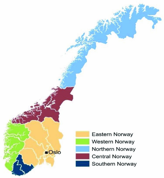
Figure A1. Five Geographic Regions of Norway
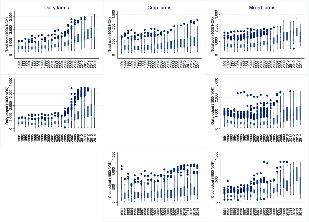
Figure A2. Box Plots across Years (1991–2014) of Total Cost per Farm (upper panels), Dairy Output (middle panels) and Crop Output (lower panels)
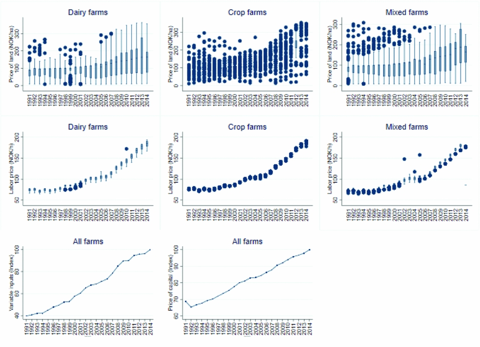
Figure A3. Box Plots across Years (1991–2014) of the Following Input Price Variables: Price of Land (upper panels) and Price of Labor (middle panels); Lower Left Panel Shows the Price of Variable Inputs (index, with no cross-sectional variation) across Years, and Lower Middle Panel Shows the Price of Capital (index, with no cross-sectional variation) across Years


 Open access