


1 Introduction
A high-power laser driver is an important part of an inertial confinement fusion (ICF) laser system, composed of a front-end, preamplifier, main amplifier, target, and other control and diagnostic systems. As an injection laser system, a nanosecond laser pulse of the front end should possess certain features, such as smooth time envelope, high contrast and beam quality. In the ICF experiment, it is required that the terminal of the high-power laser driver system can output laser pulses of different shapes in the time domain to meet the requirements of various physical experiments[Reference Temporal, Canaud, Garbett, Ramis and Weber1]. However, owing to the gain saturation effect and the main amplifier working in the near-saturation state, the gain coefficient of the main amplifier to the pulse front will be higher than that of the second half of the pulse, and the amplified laser pulse will produce distortion. To realize the specific pulse shape output at the terminal, it is required to shape the laser pulse in the front-end system. In addition, owing to the diverse requirements on the shape of the laser pulse in physical experiments, the high contrasts of the laser pulse are required for the front-end system[Reference Zheng, Wei, Zhu, Jing, Hu, Su, Zheng, Yuan, Zhou, Dai, Zhou, Wang, Xu, Xie, Feng, Peng, Guo, Chen, Zhang, Liu, Lin, Dang, Xiang and Deng2]. Contrast refers to the ratio of the peak intensity to the foot intensity of the main laser pulse. The plasma generated by the pulse can change the state of the target material, and different pulse settings can also obtain different experimental results. Therefore, the ability of high-contrast pulse time shaping is also an important index to assess the front-end system[Reference Park, Hurricane, Callahan, Casey, Dewald, Dittrich, Döppner, Hinkel, Hopkins, Pape and Ma3].
Presently, pulse shaping techniques of single longitudinal mode long pulse clipping are adopted by high-power laser facilities such as National Ignition Facility (NIF), Laser Magajoule (LMJ), Shenguang-II (SG-II), and SG-III[Reference Wisoff, Bowers, Erbert, Browning and Jedlovec4], and the pulse clipping unit includes an intensity modulator and arbitrary waveform generator (AWG). The time–power curve is easily affected by electrical noise and FM-to-AM modulation, which will have an influence on the precise calibration of the pulse shape in the feedback control system, so we need to take measures to make pulse smooth and increase the signal-to-noise ratio (SNR) in the measurement system. At present, the shaping unit mainly utilizes the cumulative average algorithm (CAA) or orthogonal matching pursuit (OMP) algorithm to enhance the pulse SNR and smoothness[Reference Huang, Lu, Jiang, Wang, Qiao and Fan5, Reference Qiao, Wang, Fan, Li, Jiang, Li, Huang and Lin6]. Although the denoising effect of the CAA is poor, and the algorithm cannot remove the FM-to-AM modulation signal so it needs a further filtering process, which has certain limitations on the recovery of a smooth pulse; OMP is affected by the complete dictionary matrix, the atomic vector of the dictionary usually uses a sine or cosine function[Reference Dileep, Dutta, Prasad and Santhosh7], and the denoising effect of a high-contrast pulse is not obvious and this algorithm has large redundancy.
In this paper, we propose a new hybrid scheme including wavelet threshold denoising (WTD) and first derivative adaptive smoothing filter (FDASF) in a closed-loop control system for smooth pulse recovery. Compared with traditional methods, WTD is determined by the nature of the wavelet transform. Based on the diversity of resolution in the wavelet transform, WTD can retain part of the original signal’s changed information. The operation speed is faster owing to the determined function model. The parameters of the traditional smoothing filter (TSF) are fixed, whereas the adaptive smoothing filter can change the parameters dynamically. It can amplify the useful signal and noise signal at the same time, enhance the edge detail information, and smooth the waveform to restrain the influence of FM-to-AM modulation. The FDASF can achieve the best effect when the noise density is not very large (<15 dB), so the preprocessing of denoising can make up for this shortcoming.
2 Principle and system structure
2.1 Structure of time pulse shaping and closed-loop control system
The time pulse shaping unit of the SG-II front-end system is shown in Figure 1. AWG is an arbitrary waveform generator, AM is amplitude modulation, and RF-AMP is the radio-frequency amplifier. Under the action of an external trigger signal and the clock, the shaping electric pulse and square wave gate pulse of AWG output are respectively loaded at the two poles of the optical waveguide modulator after amplification. Driven by these two electrical signals, the 60 ps–30 ns square-shaped laser pulse can be acquired at the output of the optical waveguide modulator to meet the requirements of physical experiments.
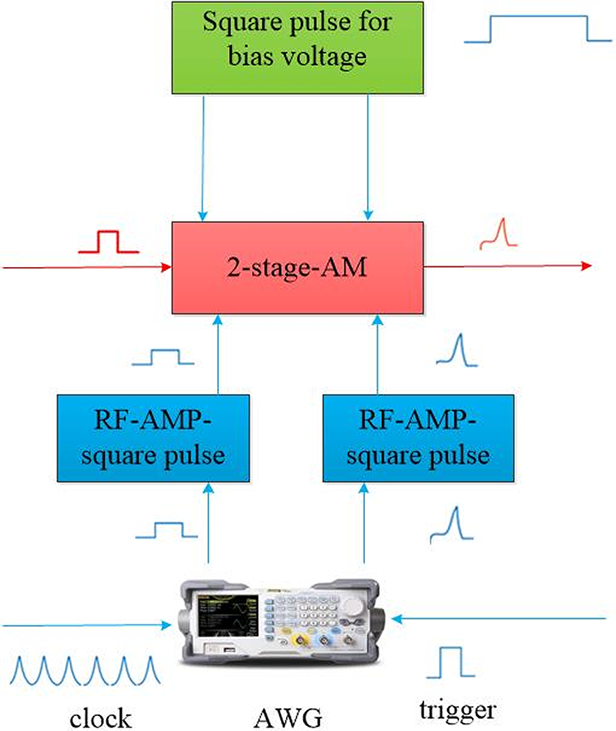
Figure 1 Schematic of the time pulse shaping unit.
Owing to the serious nonlinear effect of the electric amplifier in the system, and the time characteristic of the shaping optical pulse being controlled by the shaping electric signal, it is easy to produce large background noise, so it is necessary to design a waveform closed-loop control to compensate. To realize the closed-loop control of pulse time waveform, we use the scheme shown in Figure 2. After the output of the regenerative amplifier is sampled, the pulse waveform is measured by a photoelectric tube and a high-speed oscilloscope. The computer collects the pulse waveform data measured by the oscilloscope in real time and processes the data with a hybrid algorithm. According to the data-processing results, the computer automatically feedback controls the AWG to shape the output. The closed-loop control first calibrates the state of the shaping system, and then, according to the required regenerative output waveform, the injected pulse waveform and AWG shaped electric pulse are obtained by solving the inverse problem of regenerative amplification.

Figure 2 Schematic of the closed-loop control.
2.2 Principle of WTD
A wavelet is developed from short-time Fourier transform, which is suitable for a detailed analysis of the local components of signals. According to the theory of mathematics, a wavelet refers to the unit of orthogonal basis in space, which is a function that satisfies the condition in a certain domain. The analysis of wavelet transform is generally carried out in the space of  $\mathit{L}{(R)}^2$ (Ref. [Reference Parmod and Devanjali8]):
 \begin{align}f(t)\in L{(R)}^2\iff \int {\left|f(t)\right|}^2\mathrm{d}t<+\infty,\end{align}
where  $f(t)$ is a limited power signal and $L{(R)}^2$ is space capacity. If $\varPsi (t)\in L{(R)}^2$, satisfying the requirements of the Fourier transform, $\hat{\varPsi}(t)$ is expressed as follows:
 \begin{align}{C}_{\varPsi }=\underset{-\infty }{\overset{+\infty }{\int }}{\left|\omega \right|}^{-1}{\left|\hat{\varPsi}(t)\right|}^2\ \mathrm{d}\omega <\infty.\end{align}
 From Equation (2), we can obtain that  ${C}_{\varPsi }$ is a bounded function and $\varPsi (t)$ is a wavelet base. If the wavelet is translated or stretched, a set of wavelet sequences can be obtained, which can be expressed as follows:
 \begin{align}{\varPsi}_{a,b}(t)={\left|a\right|}^{-1/2}\varPsi \left(\frac{x-b}{a}\right),\end{align}
where a is an expansion factor and b is a translation factor. For any function, its wavelet transform can be expressed as follows:
 \begin{align}\left({W}_{\varPsi}\right)\left(a,b\right)=\left\langle f,{\varPsi}_{a,b}\right\rangle ={\left|a\right|}^{-1/2}{\int}_{\!\!-\infty}^{+\infty }f(t)\overline{\varPsi \left(\frac{t-b}{a}\right)\ \mathrm{d}t}.\end{align}
From Equation (4), we can obtain a signal that will be transformed into a two-dimensional function after continuous wavelet transform, so as to increase the intuitiveness of analysis. In the wavelet decomposition, according to different noise characteristics, the corresponding wavelet basis can be selected to denoise, which can meet the requirements of most signals. The actual signal can be expressed as
 \begin{align}\mathrm{s}(t)=g(t)+n(t),\end{align}
where  $g(t)$ and $n(t)$ are the original signal and noise signal, respectively. The ultimate goal of wavelet denoising is to reduce and suppress the noise signal and restore the original signal to the maximum extent[Reference Jenkal, Latif, Toumanari, Dliou and Biocybern9]. From the point of view of mathematical statistics, this mathematical model is a regression model about the time domain, and can also be regarded as a nonparametric estimation of $g(t)$ on an orthogonal basis. Wavelet decomposition technology is used to decompose the signal into approximate component A1 and detail component D1 at a selected scale. The low-frequency component of the signal is mainly in the approximate component, and the detail component is mainly the high-frequency component and noise. With a deeper level of decomposition, the high-frequency component of the signal is reconstructed continuously, and the denoising process of the signal is finished. In the front-end system, two-stage phase modulation is used for spectrum broadening, and the FM-to-AM conversion can be induced by the nonuniform spectral transmission and dispersion, which causes the high-frequency modulation signal and noise signal to be added on the waveform of the time pulse[Reference Tian, Zhang, Chu, Qin, Zhang, Geng, Huang, Wang and Wang10]. Because there is weak reflection on the front and back surfaces of optical elements, it is equivalent to a weak etalon with low reflectivity, and there is a certain transmittance curve for the etalon:
 \begin{align}V=1\bigg/\left(1+F{\sin}^2\frac{\delta }{2}\right),\end{align}\begin{align}F=4r/{\left(1-r\right)}^2,\end{align}
where V is transmittance, r is reflectivity, and δ is the angle of incidence. The total transmittance is the product of the transmittance of all wave plates, whereas WTD is a signal processing method based on high-frequency component decomposition. It has better applicability for this kind of signal. In this paper, the soft threshold method based on Stein unbiased likelihood estimation[Reference Tsukuma and Kubokawa11] is selected to determine the threshold. The hard threshold method is a discontinuous function. It only removes or retains the local information of the signal. After filtering, it will produce oscillation[Reference Yan, Chen, Xu, Yang and Lu12]. Compared with the hard threshold method, the soft threshold method uses parameters to achieve signal attenuation and eliminate discontinuities, so that the reconstructed signal has continuity and smoother waveform.
2.3 Principle of FDASF
The TSF can remove the noise, but it will lose many details of the signal, the most obvious of which is the edge of the signal becoming fuzzy or even distorted. The adaptive smoothing filter can remove the noise and increase the detail, so as to achieve the best smoothing effect of the signal[Reference Yang, Ye and Frossard13]. The principle of the algorithm is based on an abrupt change of the pixel gray value in the image, adaptively changing the weight of the filter, sharpening the edge of the image in the process of region smoothing, and better handling the contradiction of smoothing noise and sharpening the edge. Based on the traditional method of adaptive smoothing by difference, we propose that the first derivative processing should be carried out after the difference calculation. When the absolute value after the first-order derivation is large, it indicates that the point is a large part of jitter or curvature, which can easily form a spike, and needs to be smoothed. If the difference is small after derivation, it means that the point is part of the little jitters and does not need to be advanced[Reference Wang, Wang, Zhang, Huang, Hu, Zheng, Zhu and Deng14]. The reciprocal of the first derivative is calculated and multiplied by a correlation coefficient as the weight of the current value. The vector value weight of the previous frame after smoothing is 1. The weighted sum of the two values is used as the smoothed value. We can choose the previous point ( ${x}_0,{y}_0$) and the current point coordinate ( ${x}_1,{y}_1$). The absolute value after derivation is
 \begin{align}D=\left|\frac{\left({y}_1-{y}_0\right)}{\left({x}_1-{x}_0\right)}\right|.\end{align}
The weight of the current value is
 \begin{align}W=\frac{q}{D},\end{align}
where q is a correlation coefficient. Then the output value after filtering is as follows:
 \begin{align}{S}_{y_1}=\left({y}_0+W {y}_1\right)/\left(1+W\right).\end{align}
The FDASF works dynamically according to the weight factor. The purpose is to smooth the pulse signal and protect the detail information of the signal as much as possible. If there is too much background noise, the corresponding weight will be biased, so that the signal and noise will be amplified at the same time, resulting in signal distortion. Therefore, the hybrid algorithm can consider both denoising and detail protection to form a smooth curve[Reference Moody, Strozzi, Divol, Michel, Robey, Le Pape, Ralph, Ross, Glenzer, Kirkwood and Landen15]. In addition, the smoothing degree R can be expressed as
 \begin{align}R=\frac{\sum_{i=1}^{n-1}{\left[{h}_1\left(i+1\right)-{h}_1(i)\right]}^2}{\sum_{i=1}^{n-1}{\left[h\left(i+1\right)-h(i)\right]}^2},\end{align}
where  ${h}_1(i)$ is the smoothed signal, $h(i)$ is the original signal, and n is signal length.
3 Simulations and experimental results
3.1 Simulation results
To simulate the high-contrast time pulse waveform, periods of exponential and sinusoidal functions are synthesized in MATLAB software, and random noise is introduced to simulate the background noise in the experiment. The contrast of the simulation waveform is about 80:1. Figure 3 shows the original waveform of the simulation.

Figure 3 Original waveform of the simulation.
As shown in Figure 4, the original waveform is generated 10 times on the basis of simulated random noise, then accumulated and averaged to obtain Figure 4(a), and the OMP algorithm is used to obtain Figure 4(b). According to the results before and after denoising, the SNR is about 13 and 17 dB, respectively, by using the SNR calculation formula. The SNR of the two algorithms is low after denoising, and it is difficult to distinguish the modulated signal from the noise.

Figure 4 Time domain waveform of the simulation processed by the denoising algorithm: (a) CAA; (b) OMP.
Because there are many peaks and modulated signals in the denoising waveform, which cannot meet the needs of shaping, further filtering is required. At the same time, to highlight the advantages of the proposed adaptive smoothing filter, the denoised waveform is processed by TSF in the simulation, and the results are shown in Figure 5. It can be seen from the wrinkle degree of the ribbon graph that the smoothing degree of the denoised waveform after the CAA is only 70.1%, whereas that of the waveform denoised by the OMP algorithm is about 81.3%, and the smoothing effect is not satisfying.

Figure 5 The time domain waveform of the simulation and its corresponding ribbon graph with TSF: (a), (c) the time domain waveform and its corresponding ribbon graph using CAA and traditional filtering; (b), (d) the time domain waveform and its corresponding ribbon graph using OMP and traditional filtering.
The number of decomposition levels has a major influence on the denoising effect. Usually, if the decomposition levels are too high, and the coefficients of all layers of wavelet space are processed by threshold processing, the SNR will be reduced; if the decomposition level is too small, the denoising effect will be ignored and the SNR will not be improved. As shown in Figure 6, we denoise the waveform in Figure 3 with different decomposition scales and estimate the SNR. From the results, we can see that the fifth level decomposition is the best. Therefore, for this kind of signal, the fifth level wavelet decomposition is most suitable in WTD.

Figure 6 The denoising results with WTD under different decomposition levels.
For the new hybrid shaping scheme of WTD and FDASF in this paper, the results are shown in Figure 7. From the graph, the SNR obtained by WTD is about 30 dB. This is much higher than the CAA and OMP algorithm. It can be seen from the detail enlarged image that the background noise can be removed and the modulated signal can be restored. From the wrinkle degree of the ribbon graph, the smoothness after adaptive smoothing filter is about 98.8%, and the waveform has no ripple modulation, which can meet the needs of time pulse shaping. Therefore, in the experiment, the scheme proposed in this paper is selected for recovery.

Figure 7 The time domain waveform of the simulation and its corresponding ribbon graph with the new hybrid shaping scheme: (a) the time domain waveform using WTD; (b) the time domain waveform using FDASF after WTD; (c) ribbon graph using FDASF after WTD.
3.2 Experimental results
In the experimental step, according to the structure of Figure 2, the signal is collected after the preamplifier system of the injection laser system of the SG-II facility, and the algorithm is processed by the computer. The output is measured by a high-speed photo-detector (Newport, 1014) and a 30 GHz oscilloscope (Agilent, DSO93004L) at 80 GHz sampling. To reflect the applicability of the proposed shaping algorithm, we collect and process two different contrast waveforms for shooting. First, the common pulse waveform is processed, and the processing result is shown in Figure 8. The SNR increased to 33 dB by denoising the collected ordinary pulse waveform. The noise and modulation signals can be separated obviously, and the smooth curve can be obtained after adaptive filtering process, which can meet the requirements of shaping. The smoothness can be estimated to be about 98.7% from the wrinkle degree of the ribbon graph.

Figure 8 The time domain waveform of the experiment and its corresponding ribbon graph obtained by the new hybrid shaping scheme: (a) original waveform of the experiment; (b) the time domain waveform using WTD; (c) the time domain waveform using FDASF after WTD; (d) ribbon graph using FDASF after WTD.
We collect the high-contrast time domain waveform of the experiment in the oscilloscope. As shown in Figure 9, the SNR increased to about 30 dB by denoising the collected ordinary pulse waveform, and the smoothness can be estimated to be about 99.2% from the wrinkle degree of the ribbon graph.

Figure 9 The high-contrast time domain waveform of the experiment and its corresponding ribbon graph obtained by the new hybrid shaping scheme: (a) original waveform of the experiment; (b) the time domain waveform using WTD; (c) the time domain waveform using FDASF after WTD; (d) ribbon graph using FDASF after WTD.
4 Discussion
4.1 Comparative analysis of denoising algorithms
It can be seen that the SNR obtained by the WTD algorithm is higher than that of CAA algorithm and OMP algorithm. For the CAA, only the signals collected several times are superimposed and averaged[Reference Montgomery16]. The denoising effect is related to the number of times of accumulation, and the average times are affected by the sampling rate of the oscilloscope. It can only suppress some random noise without reconstruction and decomposition of the algorithm and the algorithm cannot suppress the modulated signal, so it has great limitations. For OMP algorithm, it is given over the complete dictionary matrix  $P\in {R}^{n\times k}$, and each column represents the atom of a prototype signal. Given a signal y, it can be expressed as a sparse linear combination of these atoms:
 \begin{align}\mathrm{y}=P\cdot x=\sum_k{\phi}_k\cdot {x}_k={y}_{\mathrm{omp}},\end{align}
where P is over the complete dictionary, x is an atom,  ${\phi}_k$ is a sparse matrix, and ${y}_{\mathrm{omp}}$ is a signal after denoising. The problem of sparse representation is how to find the sparsest x when y and P are known, so the generation of the dictionary matrix directly affects the final denoising effect. For continuous smooth signal denoising, a Fourier basis can be used for sparse representation, but for high-power laser physics experiments, the complexity of the pulse shape is different, especially for a high-contrast pulse; their eigenvectors will be more complex, more basis vectors need to be added to the dictionary matrix, and the bottom noise of each optical device and electrical device also needs to be calibrated, which make the dictionary matrix more complete. Therefore, if a more complete dictionary library cannot be built, the denoising level of OMP algorithm will be limited.
The WTD proposed in this paper is based on the decomposition of a selected scale into approximate component A1 and detail component D1 of the scale[17–19]. The low-frequency component of the signal is mainly in the approximate component, and the detail component is mainly composed of the high-frequency component and noise. With a deeper level of decomposition, the high-frequency components of the signal are continuously reconstructed, and the denoising process of the signal is finished, that is, the signal is divided into low-frequency and high-frequency components from the frequency domain and processed separately. In the front-end system, the signal generated by the seed pulse module needs to enter the cascaded phase modulator module with modulation frequency of 3 and 20 GHz, respectively. Among them, 3 GHz phase modulation broadens the spectrum to 0.1 nm, which is used to suppress stimulated Brillouin scattering effect of the large-aperture quartz element, whereas 20 GHz phase modulation broadens the spectrum to 0.3 nm to meet the bandwidth requirements of smoothing by spectral dispersion. An FM-to-AM modulation signal will be added on the waveform of the time pulse, and the characteristic of the wavelet threshold algorithm is analyzing the signal under high-frequency decomposition conditions, so it has better applicability for this kind of signal[20–22].
In addition, the WTD proposed in this paper is a soft threshold method based on unbiased likelihood estimation, which selects the appropriate threshold through minimum risk estimation. The threshold function is mainly divided into a hard threshold and a soft threshold, of which the hard threshold  ${s}_1$ can be expressed as
 \begin{align}{\mathit{s}}_1=\left\{\!\!\begin{array}{c}k,\left|k\right|>T,\\{}0,\left|k\right|\le T,\end{array}\right.\end{align}
and the soft threshold  ${s}_2$ is
 \begin{align}{s}_2=\left\{\!\!\begin{array}{l}\operatorname{sign}(k)\left(\left|k\right|-T\right),\left|k\right|>T,\\{}0,\left|k\right|\le T,\end{array}\right.\end{align}
where k is the original signal and T is the threshold. Compared with the above two formulas, the hard threshold method is a discontinuous function. It only removes or retains local information of the signal. After filtering, it will produce oscillation. The soft threshold method uses parameters to realize the attenuation of the signal, eliminates the discontinuities, makes the reconstructed signal consecutive and smoother, and is more conducive to the later filtering and shaping processes[23–25]. For the decomposition level, it is related to signal length, signal characteristics, and sampling rate. In the future research, we will use self-adaptive WTD to improve the ability of denoising.
4.2 Comparative analysis of smoothing filtering
The basic principle of a smoothing filter is selecting the median value of each pixel value in a neighborhood of the pixel and using a processed pixel to replace the unprocessed pixel. Its main function includes that the gray value of the pixel is close to the surrounding pixels, thus eliminating the isolated noise points, so the filter can effectively restrain salt and pepper noise. However, the effect of the TSF is greatly affected by the size of the filtering window. There is a contradiction between eliminating noise and protecting the details of the image: if the filtering window is small, it can well protect some details in the image, but the filtering effect on the noise is not very satisfying; in contrast, the larger window size has better noise filtering effect, but it will cause certain fuzzing in the image. Therefore, the window size of conventional smoothing filter is fixed, and it cannot take into account the details of denoising and waveform protection at the same time. The FDASF proposed in this paper is based on the derivative of the current sampling point and the previous sampling point to smooth. If the object has normal motion, its first derivative and curvature are also in a stable state, and the curve must be smooth. However, the jitter is instantaneous and has a large offset from the normal position, which will form a peak on the curve, and change the first derivative and curvature continuously. For this adaptive algorithm, if the signal has large noise (>15 dB), it will affect the calculation of the derivative and the parameter transformation of the filter. Therefore, the denoising is used to compensate before smoothing to achieve the best effect. In the next step, we will calibrate the photoelectric converter, oscilloscope, AWG and other devices, and then optimize the algorithm parameters.
5 Conclusion
Aiming at the shaping technology of high-power laser driver front-end system for complex time shape seed pulse, we report a hybrid smooth pulse recovery scheme including WTD and FDASF in a closed-loop control system. Simulation and experimental results show that compared with the CAA and OMP denoising algorithm combined with TSF, the new scheme can be used to obtain the time–power curve with an SNR of 30 dB and smoothness of 98.8%. By adopting these two algorithms simultaneously, the system can output a time–power curve with higher SNR and smoother level, as well as provide enhanced control and management capabilities for pulse shaping techniques. We believe that the proposed scheme can promote the calibration accuracy of the time–power curve in the front-end system of high-power laser devices.
Funding
This work was supported by the Strategic Priority Research Program of the Chinese Academy of Sciences (No. XDA25020303).


 Open access