


1. Introduction
The chemical oxygen–iodine laser (COIL) has been an important research and technology since the first successful demonstration in 1977[Reference McDermott, Pchelkin, Benard and Bousek1]. The COIL is unique among chemical lasers because it is the only chemical laser to utilize electronic transitions rather than vibrational transitions[Reference Rittenhouse, Phipps and Helms2]. The characteristics, such as good atmospheric propagation, short wavelength and excellent transmission through optical fibers, make the COIL a good candidate for high-power laser applications. Simulation of chemical lasers such as the COIL is of timely interest due to the recent acceleration of the military development programme[Reference Lamberson3] and ongoing commercial development programmes[Reference Carroll, King, Fockler, Stromberg, Solomon and Sentman4–Reference Yoshida and Shimizu6]. Although seemingly separated by diverse goals, a common element shared by these research and development programmes is the need to understand the physics underlying the COIL so that its performance with respect to the specific mission may be optimized.
The COIL presents a significant challenge to analytical modeling. Disparate physical processes including transverse injection of secondary gases, molecular diffusion, subsonic flow, transonic flow, supersonic flow, non-equilibrium chemical reactions, heat release, shock waves and stimulated emission of photons all occur within the COIL. The light in an optical resonator downstream of the nozzle blades is amplified by the stimulated emission from excited iodine atoms I(2P1/2), and undergoes diffraction, which causes power loss and refraction due to the presence of a nonuniform density distribution in the resonator. Otherwise, species redistribution and heat release occur in the flow due to the stimulated emission of photons. A complete mathematical model of the physical processes within the COIL therefore requires a 3D description of the fluid dynamics and continuity of multiple species coupled to descriptions for molecular transport processes, chemical kinetics and radiation transport.
Buggeln et al.[Reference Buggeln, Shamroth, Lampson and Crowel7] coupled the Fabry–Perot resonator model with the three-dimensional (3D) Navier–Stokes equations and modeled the region from the injectors to the cavity where the power extraction occurs over a microscale domain. Lampson et al.[Reference Lampson, Plummer, Erkkila, Crowell and Helms8,Reference Lampson, Plummer, Crowell and Helms9] investigated laser beam quality issues with 3D Navier–Stokes (MINT) and wave optics (OCELOT) codes. The premixed flow assumption was used in the cavity flow field simulation coupling with wave optics over a macroscale domain, and the iodine dissociation rate constant was increased to match the nozzle exit plant dissociation fraction[Reference Lampson, Plummer, Erkkila, Crowell and Helms8,Reference Lampson, Plummer, Crowell and Helms9] .
Hishida et al.[Reference Hishida, Azami, Iwamoto, Masuda, Fujii, Atsuta and Muro10] simulated the flow and optical fields of a supersonic COIL by coupling the three-dimensional Navier–Stokes equations and the paraxial wave equation together. The solution obtained in the mixing/reacting calculation microscale domain is used assuming symmetry to generate the upstream boundary condition of the cavity calculation macroscale domain ignoring the effects of boundary layers and diverging walls[Reference Hishida, Azami, Iwamoto, Masuda, Fujii, Atsuta and Muro10].
Wu et al.[Reference Wu, Huai, Jia and Jin11,Reference Wu, Huai, Jia and Jin12] studied the flow and optical fields of a supersonic COIL by coupling the three-dimensional Navier–Stokes equations and the paraxial wave equation together within the whole laser cavity. The results[Reference Wu, Huai, Jia and Jin11,Reference Wu, Huai, Jia and Jin12] do not show any mixing and nozzle tail flow effect imprints on the flow or optical fields as seen in[Reference Lampson, Plummer, Erkkila, Crowell and Helms8,Reference Lampson, Plummer, Crowell and Helms9] ; perhaps the grid is not fine enough to resolve them.
Although these studies have shown reasonable comparisons with measured gain, power and dissociation data[Reference Buggeln, Shamroth, Lampson and Crowel7–Reference Wu, Huai, Jia and Jin12], they have provided incomplete insight into some of the fluid dynamic effects within COIL flow fields.
The focus of this paper is to propose a more exact modeling of lasing in the COIL medium coupling with the effects induced by transverse injection of secondary gases, non-equilibrium chemical reactions, nozzle tail flow and boundary layer. The coupled steady solutions of the fluid dynamics and optics in a COIL complex three-dimensional cavity flow field are obtained following the proposal. The modeling results are given, and a summary and conclusions are also presented.
2. The proposal on more exact modeling of COIL laser performance
2.1. Modeling approach
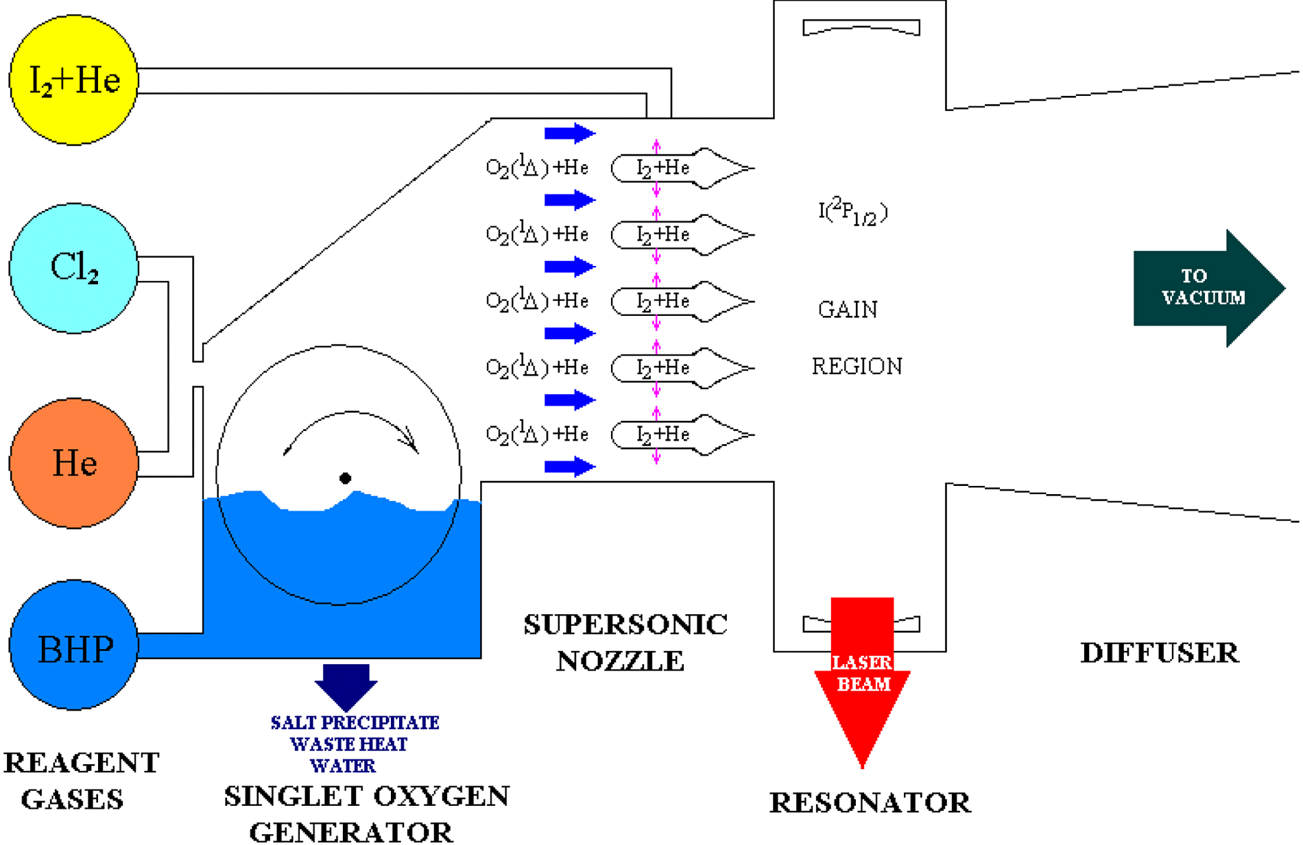
The laser system analyzed in this paper is a Roto COIL-like laser[Reference Buggeln, Shamroth, Lampson and Crowel7]. A lot of supersonic nozzle blades are used (see Figures 1 and 2). The subsonic flow entering the nozzle consists of He and products from the  ${\text{O} }_{2} ({\text{} }^{1} \hspace {-2.5pt} \mathrm{\Delta} )$ generator which include ${\text{O} }_{2} \mathop{(}\nolimits ^{1} \hspace {-2.5pt} \mathrm{\Delta} )$, ${\text{O} }_{2} \mathop{(}\nolimits ^{3} \hspace {-2.5pt} \mathrm{\Sigma} )$, ${\text{H} }_{2} \text{O} $ and ${\text{Cl} }_{2} $. As the flow travels in a constant area section toward the nozzle throat, a sonic secondary mixture of ${\text{I} }_{2} $ and He is injected normal to the flow through a lot of orifices from the nozzle blades’ walls, shown in Figure 2. The now mixing/chemically reacting flow is choked and rapidly expanded to a Mach number of approximately $M= 2$, static pressures below $p= 6$ torr, and temperatures below $T= 200~\text{K} $. After the rapid expansion, the flow enters the optical cavity, where the mirrors are placed and photons are extracted from the flow. Further downstream from the cavity the pressure is recovered and the flow exhausted.
Many factors influence laser performance, such as resonator configuration, resonator optics, gain medium, tunnels and optical boxes, residual alignment error, and so on. Some analyses[Reference Bhowmik, Yang and Jones13,Reference Boreisho, Mal’kov and Savin14] show that the contribution of the gain medium is most significant.
The gas flow in a chemical laser such as a COIL is characterized by a low Reynolds’ number and contains all the features typical of supersonic motion of a viscous gas: large boundary layers and shock and expansion waves from nozzle contours and cavity wall. The flow field structure is also complicated by both mixing and reaction processes of oxygen and iodine flows that have different thermodynamic and optical properties and by heat generation resulting from chemical reaction. If the diffuser design were not to provide enough pressure recovery and good cavity isolation for a COIL, the effects of adverse pressure gradients influencing the flow within the cavity could not be neglected. These phenomena determine the gas dynamic homogeneity of the COIL active medium.
Because the description of a high-energy laser cavity involves a large number of variables, i.e., density, pressure, species and OPD (optical path length difference) profiles, it is difficult to assess their impact analytically. To achieve even the basic medium homogeneity requirements of an ideal cavity, 3D CFD (computational fluid dynamics) codes are necessary.
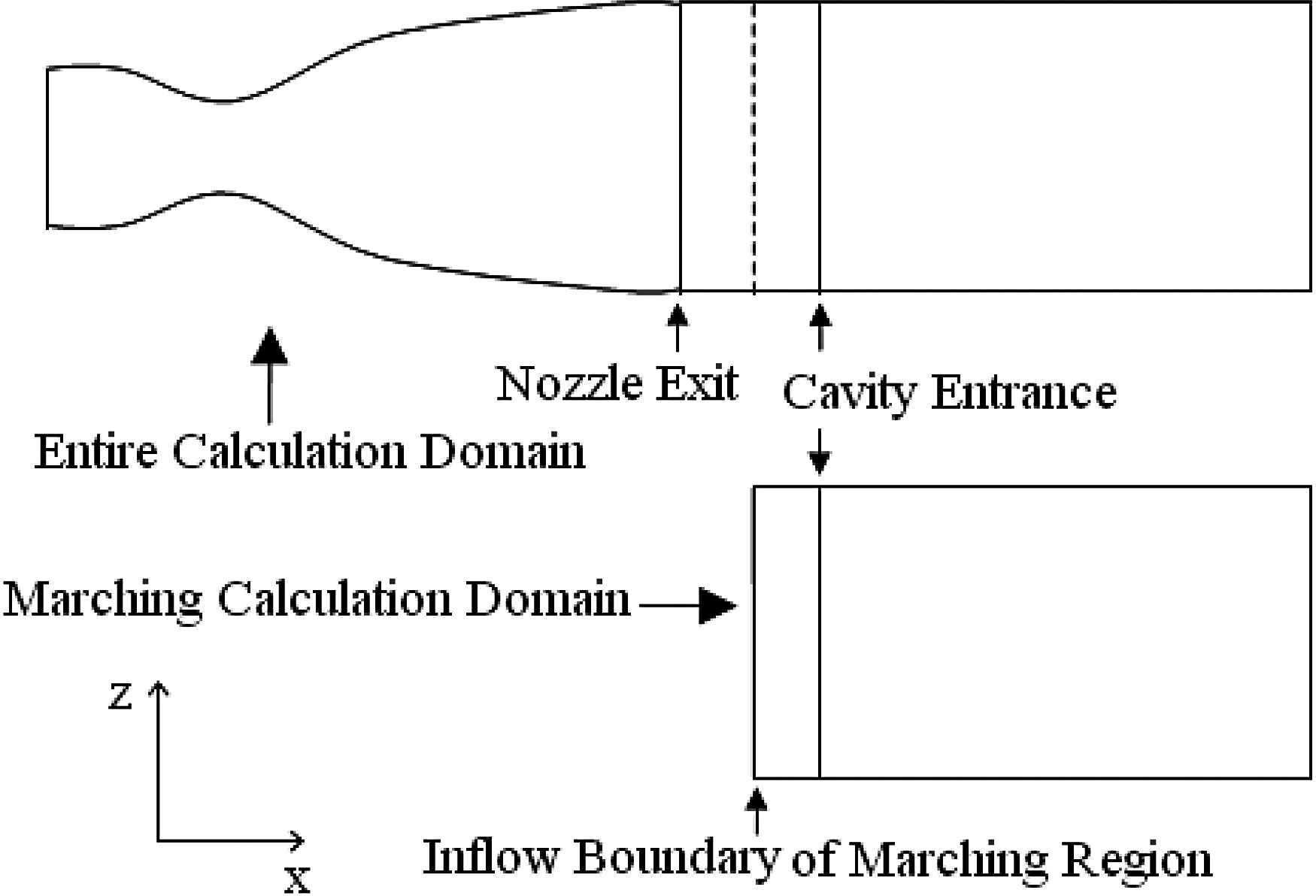
With the experimental diagnostics performed upstream of the mixing nozzle and in the I2 plenum, the thermodynamic state and composition of the flows entering the mixing nozzle are known. The flow in the cavity is assumed to be supersonic, so physical boundary conditions are imposed at the inflow but not the outflow. However, finite-difference equations usually require additional boundary conditions that would overspecify the differential problem, and so does in this paper. But if there are enough cells in the flow direction, the numerical outflow boundary effects are negligible. However, if the effects of adverse pressure gradients influencing the flow within the cavity could not be neglected, the back pressure condition would be adopted for the outflow boundary. Thus it is assumed possible to simulate the details of the flow field within the mixing nozzle and cavity alone without detailed simulations of the generator and pressure recovery systems. Furthermore, the spatial marching method[Reference Farmer and Ramshaw15] for steady-state supersonic flow would be adopted to separate the nozzle and resonator flow calculations. The nozzle flow calculation is performed first, and the steady-state outflow conditions from nozzle flow calculation is processed and converted into inflow boundary conditions for the resonator flow calculations.
The smallest length scale which characterizes the problem is the diameter of the iodine injection hole, and the largest one is the gain length. The computational effort to calculate the flow field over the entire nozzle bank with a grid fine enough to resolve the injection holes is so large as to preclude doing the calculation. Therefore, the problem must be broken down into smaller problems which are computationally manageable. Two options are available. The first is to simulate the entire system at a sufficiently reduced level of spatial detail to make the problem computationally tractable. The second option is to simulate a representative subdomain of the COIL flow field at a sufficiently high level of detail to capture the details of the mixing and reacting processes. The question of what level of detail is required essentially reduces to how important the fluid dynamics of the mixing processes are within the context of the system as a whole.

Figure 1. Schematic of a chemical oxygen–iodine laser.
Figure 2. Schematic of nozzle and cavity geometry.
2.2. Governing equations for the flow field
Water vapor is produced in the chemical oxygen generator as an undesirable by-product. For simplicity, the condensation of water vapor due to the supersonic cooling is ignored in the present calculation. As the Reynolds number of the S-COIL is only of the order of  $1{0}^{2} $– $1{0}^{4} $, the flow is likely to remain laminar, and viscous effects will dominate the nozzle–cavity flow field. Moreover, the compressibility and the rapid acceleration by the nozzle tend to stabilize the flow.
Based on the above assumptions, the governing equations, the full Navier–Stokes equations with a detailed chemistry mechanism, are given in the following form:
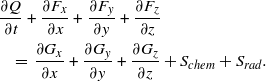 $$\displaystyle \frac{\partial Q}{\partial t} + \frac{\partial {F}_{x} }{\partial x} + \frac{\partial {F}_{y} }{\partial y} + \frac{\partial {F}_{z} }{\partial z} \quad = \,\frac{\partial {G}_{x} }{\partial x} + \frac{\partial {G}_{y} }{\partial y} + \frac{\partial {G}_{z} }{\partial z} + {S}_{chem} + {S}_{rad} .$$
 In this equation, the conservative vector  $Q$, the convection and viscous terms $F$ and $G$ in the $x, y$ and $z$ directions, the source term related to the chemical reaction ${S}_{chem} $ and the source term related to the radiative flux ${S}_{rad} $ are
$$\begin{eqnarray}\displaystyle Q= \left( \begin{array}{ @{}l@{}} \displaystyle \rho \\ \displaystyle \rho u\\ \displaystyle \rho v\\ \displaystyle \rho w\\ \displaystyle E\\ \displaystyle {\rho }_{i} \end{array} \right), \quad {F}_{x} = \left( \begin{array}{ @{}l@{}} \displaystyle \rho u\\ \displaystyle \rho {u}^{2} + p\\ \displaystyle \rho uv\\ \displaystyle \rho uw\\ \displaystyle (E+ p)u\\ \displaystyle {\rho }_{i} u\end{array} \right), \\\displaystyle {F}_{y} = \left( \begin{array}{ @{}l@{}} \displaystyle \rho v\\ \displaystyle \rho uv\\ \displaystyle \rho {v}^{2} + p\\ \displaystyle \rho vw\\ \displaystyle (E+ p)v\\ \displaystyle {\rho }_{i} v\end{array} \right), \quad {F}_{z} = \left( \begin{array}{ @{}l@{}} \displaystyle \rho w\\ \displaystyle \rho uw\\ \displaystyle \rho vw\\ \displaystyle \rho {w}^{2} + p\\ \displaystyle (E+ p)w\\ \displaystyle {\rho }_{i} w\end{array} \right), \\\displaystyle {S}_{chem} = \left( \begin{array}{ @{}l@{}} \displaystyle 0\\ \displaystyle 0\\ \displaystyle 0\\ \displaystyle 0\\ \displaystyle 0\\ \displaystyle {\dot {w} }_{c, i} \end{array} \right), \quad {S}_{rad} = \left( \begin{array}{ @{}l@{}} \displaystyle 0\\ \displaystyle 0\\ \displaystyle 0\\ \displaystyle 0\\ \displaystyle - g\tilde {I} \\ \displaystyle {\dot {w} }_{r, i} \end{array} \right), \\\displaystyle {G}_{x} = \left( \begin{array}{ @{}c@{}} \displaystyle 0\\ \displaystyle {\tau }_{xx} \\ \displaystyle {\tau }_{xy} \\ \displaystyle {\tau }_{xz} \\ \displaystyle u{\tau }_{xx} + v{\tau }_{xy} + w{\tau }_{xz} + {q}_{x} \\ \displaystyle {J}_{x} \end{array} \right)\quad , \displaystyle \\\displaystyle {G}_{y} = \left( \begin{array}{ @{}c@{}} \displaystyle 0\\ \displaystyle {\tau }_{yx} \\ \displaystyle {\tau }_{yy} \\ \displaystyle {\tau }_{yz} \\ \displaystyle u{\tau }_{yx} + v{\tau }_{yy} + w{\tau }_{yz} + {q}_{y} \\ \displaystyle {J}_{y} \end{array} \right), \displaystyle \\\displaystyle {G}_{z} = \left( \begin{array}{ @{}c@{}} \displaystyle 0\\ \displaystyle {\tau }_{zx} \\ \displaystyle {\tau }_{zy} \\ \displaystyle {\tau }_{zz} \\ \displaystyle u{\tau }_{zx} + v{\tau }_{zy} + w{\tau }_{zz} + {q}_{z} \\ \displaystyle {J}_{z} \end{array} \right)\end{eqnarray}$$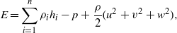 $$\displaystyle E= \sum _{i= 1}^{n} \rho _{i}{h}_{i} - p+ \frac{\rho }{2} ({u}^{2} + {v}^{2} + {w}^{2} ), \displaystyle$$
 where  $\rho $, $u, u, w$ and $p$ denote the density, the velocities in the $z, y$ and $z$ directions and the pressure of the mixture, $g$ the gain coefficient, $\tilde {I} $ the radiative flux, $\rho $ ${}_{i} $ the mass concentration and ${h}_{i} $ the enthalpy of $i\text{th} $ species, $\tau $ the viscous stress, $q$ the heat flux due to heat conduction and diffusion and $J$ the diffusion flux, respectively. To evaluate the $i\text{th} $ species production rate due to chemical reaction ${\dot {w} }_{c, i} $ in Equation (2), a chemical kinetic model[Reference Madden and Solomon16] encompassing 13 chemical reactions and 10 chemical species is used in the present calculation.
The  $i\text{th} $ species production rate due to the stimulated emission in Equation (2) ${\dot {w} }_{r, i} $ is
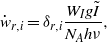 $${\dot {w} }_{r, i} = {\delta }_{r, i} \frac{{W}_{I} g\tilde {I} }{{N}_{A} h\nu } ,$$
 where  ${\delta }_{r, i} = - 1$ if the $i\text{th} $ species is I(2P1/2), ${\delta }_{r, i} = 1$ if the $i\text{th} $ species is I(2P3/2); ${\delta }_{r, i} = 0$ for other species. In Equations (2) and (3), ${W}_{i} $ denotes the molecular weight, ${N}_{A} $ is Avogadro’s number and $h\nu $ is the photon energy. The gain coefficient $g$ is evaluated by
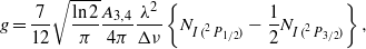 $$g= \frac{7}{12} \sqrt{\frac{\ln 2}{\pi } } \frac{{A}_{3, 4} }{4\pi } \frac{{\lambda }^{2} }{\Delta \nu } \left\{{N}_{I\mathop{(}\nolimits ^{2} {P}_{1/ 2} )} - \frac{1}{2} {N}_{I\mathop{(}\nolimits ^{2} {P}_{3/ 2} )} \right\},$$
 where  $N$ is the number density of each species, ${A}_{3, 4} $ the Einstein coefficient for the 3–4 transition, $\lambda = 1. 315~\mathrm{\mu} \text{m} $ and $\Delta \nu $ is the Doppler line width. If there no lasing in the flow, such as the nozzle flow case, $I= 0$, the source term related to the radiative flux ${S}_{rad} $ vanishes.
2.3. Governing equations for the optical field
The radiative flux  $\tilde {I} $ is determined by solving the paraxial wave equation:
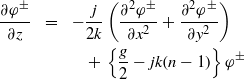 $$\displaystyle \frac{\partial {\varphi }^{\pm } }{\partial z} = \displaystyle - \frac{j}{2k} \left(\frac{{\partial }^{2} {\varphi }^{\pm } }{\partial {x}^{2} } + \frac{{\partial }^{2} {\varphi }^{\pm } }{\partial {y}^{2} } \right)+ \,\left\{\frac{g}{2} - jk(n- 1)\right\}{\varphi }^{\pm }$$
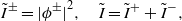 $$\displaystyle {\tilde {I} }^{\pm } = \mathop{\vert {\phi }^{\pm } \vert }\nolimits ^{2} , \quad \tilde {I} = {\tilde {I} }^{+ } + {\tilde {I} }^{- } , $$
 where  ${\phi }^{\pm } $ denotes the two-way complex amplitude and $k$ the wavenumber. The refractive index of the gas mixture $n$ in Equation (5) is determined by the Lorentz–Lorenz relation[Reference Swift, Schlie and Rathge17]:
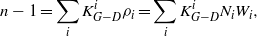 $$n- 1= \sum _{i}{ K}_{G- D}^{i} {\rho }_{i} = \sum _{i}{ K}_{G- D}^{i} {N}_{i} {W}_{i} ,$$
 where  ${ K}_{G- D}^{i} $ is Gladstone–Dale constant for species $i$ at wavelength $1. 315~\mathrm{\mu} \text{m} $.
Then, the flow and optical fields are simulated by solving the Navier–Stokes equations (1) and the wave equation (5) simultaneously. The governing equations (1) in the physical domain are transformed to the computational domain and discretized with the cell-centered finite volume method. The paraxial wave equation (5) in the  $z$ direction is divided into two parts: the diffraction part and the amplification and refraction part. The diffraction part is solved using a fast Fourier transform method; then the analytical solution for the remaining part is multiplied to that[Reference Sziklas and Siegman18].
2.4. Inflow boundary conditions for resonator flow calculations
The focus of this paper is to propose a more exact modeling of lasing in the COIL medium, and lasing occurs only in the resonator. Therefore, the cavity flow calculation could be performed alone, if the inflow boundary conditions could be set exactly.
To set the inflow boundary conditions exactly, two scale calculations are performed[Reference Lampson, Plummer, Erkkila, Crowell and Helms8] (see Figure 3). The microscale calculation includes the influence of the injector holes array and shock waves from the nozzle blades but ignores the presence of the nozzle endwall. The macroscale calculation includes shock waves and boundary layers associated with the nozzle bank sidewall but ignores the mixing of the injected iodine with the primary flow. The steady-state outflow boundary condition obtained in the microscale calculation domain is used assuming periodicity to generate the average upstream boundary condition of the cavity flow calculation domain (see Figure 4). And the steady-state unitary variable distributions with the corresponding average values on the outflow boundary obtained in the macroscale calculation domain are used as the unitary variable distributions on the upstream boundary of cavity flow calculation domain. Thus, the steady-state outflow boundary conditions obtained in both the microscale calculation domain and the macroscale calculation domain are processed and converted into inflow boundary conditions for the resonator flow calculations. Therefore, the effects induced by transverse injection of secondary gases, non-equilibrium chemical reactions, nozzle tail flow and boundary layer are coupled to the inflow boundary conditions for the resonator flow calculations, and consequently to the resonator flow calculations.
Figure 3. Microscale and macroscale computational domains.
Figure 4. Schematic of the microscale computation processed and converted into inflow boundary conditions for the macroscale computational domains.
2.5. Methodology of laser performance simulation
In order to simulate the entire resonator, the gain/intensity sheet concept[Reference Lampson, Plummer, Erkkila, Crowell and Helms8] is adopted (see Figure 5). In order to simulate the cavity flow field more accurately, each gain/intensity sheet is corresponding to a 3D macroscale flow calculation over domain  $H\times W$. The influence of the intensity variation in the optical axis direction is incorporated in the gain sheet model where the fluid dynamics calculation between each set of nozzle blades is assumed to be independent of the adjacent blades (i.e., the intensity field varies ‘slowly’ over the distance $W$ between blades). The gain/intensity sheet is the mechanism which links the gain and OPD field calculated by the Navier–Stokes equations solver to the wave equation solver which, in turn, calculates the corresponding intensity field. This intensity field is then passed back to the Navier–Stokes equations solver to complete the iteration loop. The process is continued iteratively until a steady state is achieved, and the field no longer changes from one iteration to the next (within a prescribed tolerance). The gain/OPD sheet is a two-dimensional (2D) array obtained from the 3D macroscale calculation by averaging the gain and OPD over the length $W$. The path length associated with this gain sheet which determines the total OPD and ${g}_{0} L$ product for the sheet is determined by dividing the total resonator one-way gain length by the number of gain/intensity sheets selected for the problem. The resonator configuration analyzed in this paper is a positive branch unstable resonator.
Figure 5. Unstable resonator configuration with multiple macroscale computational domains showing the gain sheet approach.
3. Calculation results
3.1. Demonstration of marching computation
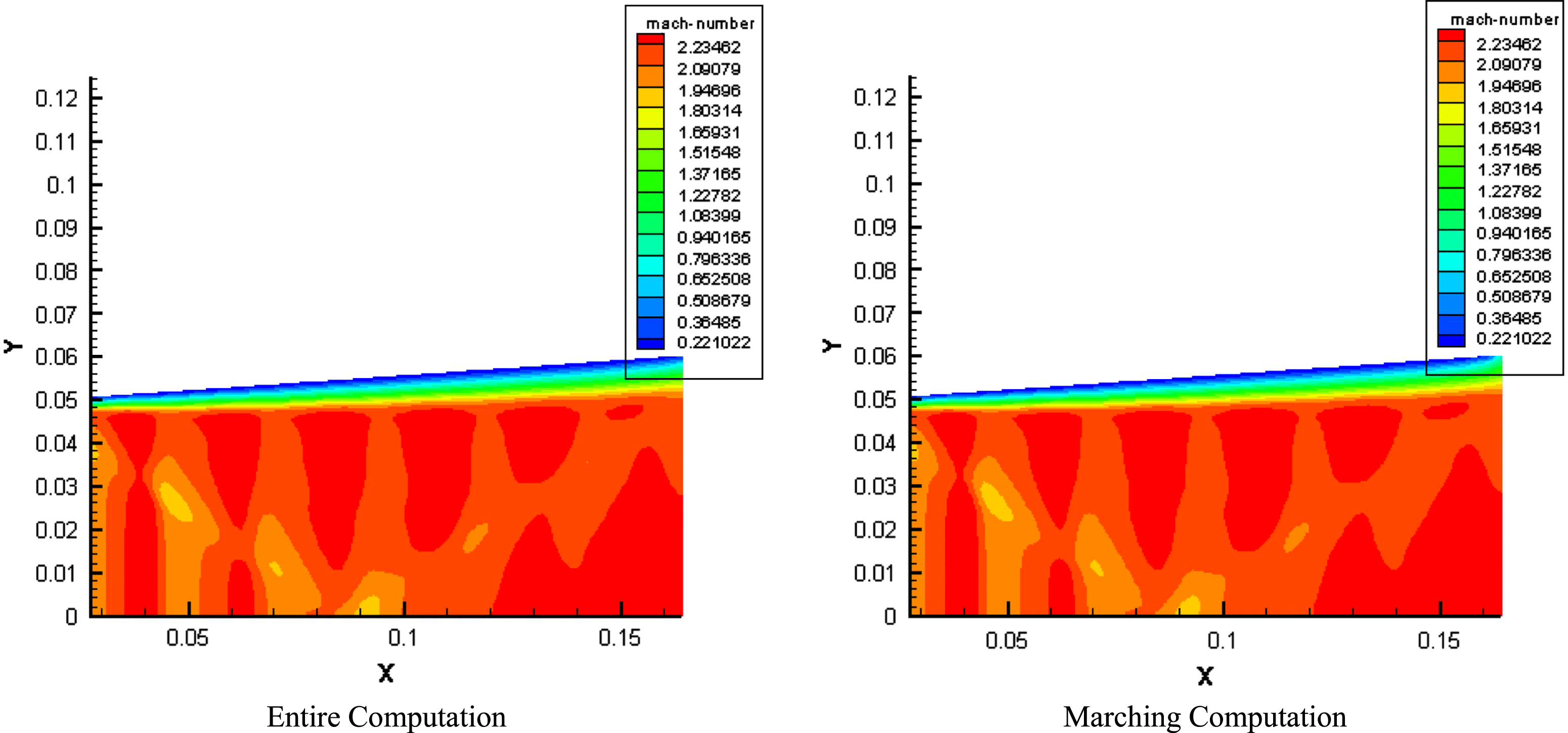
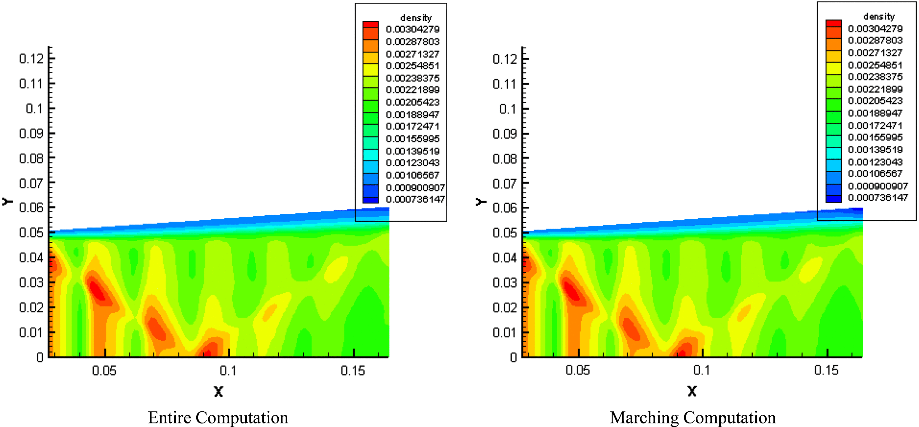
In order to demonstrate the validity of the spatial marching method used in our calculation, two cases of computational domains are simulated: one is the entire computational region including the nozzle and cavity over domain  $H\times W$, and the other is the marching computational region just including the cavity over domain $H\times W$ (see Figure 6). The premixed assumption is used in the two calculations. No-slip boundary conditions are used for the solid walls and the wall temperatures are set to $29{8}^{\circ } ~\text{K} $. Symmetry boundary conditions are used on all three symmetry planes and the pressure is fixed at the outflow boundary of the cavity. For the entire computation, the inflow boundary is set as a subsonic inflow boundary. But for the marching computation, the inflow boundary is set as a supersonic inflow boundary, where fluid variables remain frozen at their steady values from the entire computation at the same position. The steady-state flow fields are obtained in the two calculations.
Figure 6. Schematic of the entire/marching computational domains.
In Figures 7 and 8, the results obtained in the entire computational domain and the marching computational domain are compared with each other. Figures 7 and 8 show that both the variables’ contours and values are almost the same in the two computations. This indicates that the marching method is applicable in our calculation with high precision. Therefore, to avoid recalculating the nozzle flow field for each gain sheet, the calculation could be split into two parts: a nozzle flow field calculation which extends from just upstream of the large I2 injection hole to the nozzle exit plane and a laser cavity calculation which extends from the nozzle exit plane to the downstream end of the mirror. The nozzle flow field provides the initial condition for the laser cavity calculation and need only be calculated once for a given set of flow conditions. In addition, by splitting up the region into two parts, the amount of computer time required to perform such calculations is greatly reduced.
Figure 7. The predicted Mach number distributions at a plane normal to the optical axis.
Figure 8. The predicted density distributions at a plane normal to the optical axis.
3.2. Flow field downstream of nozzle blades
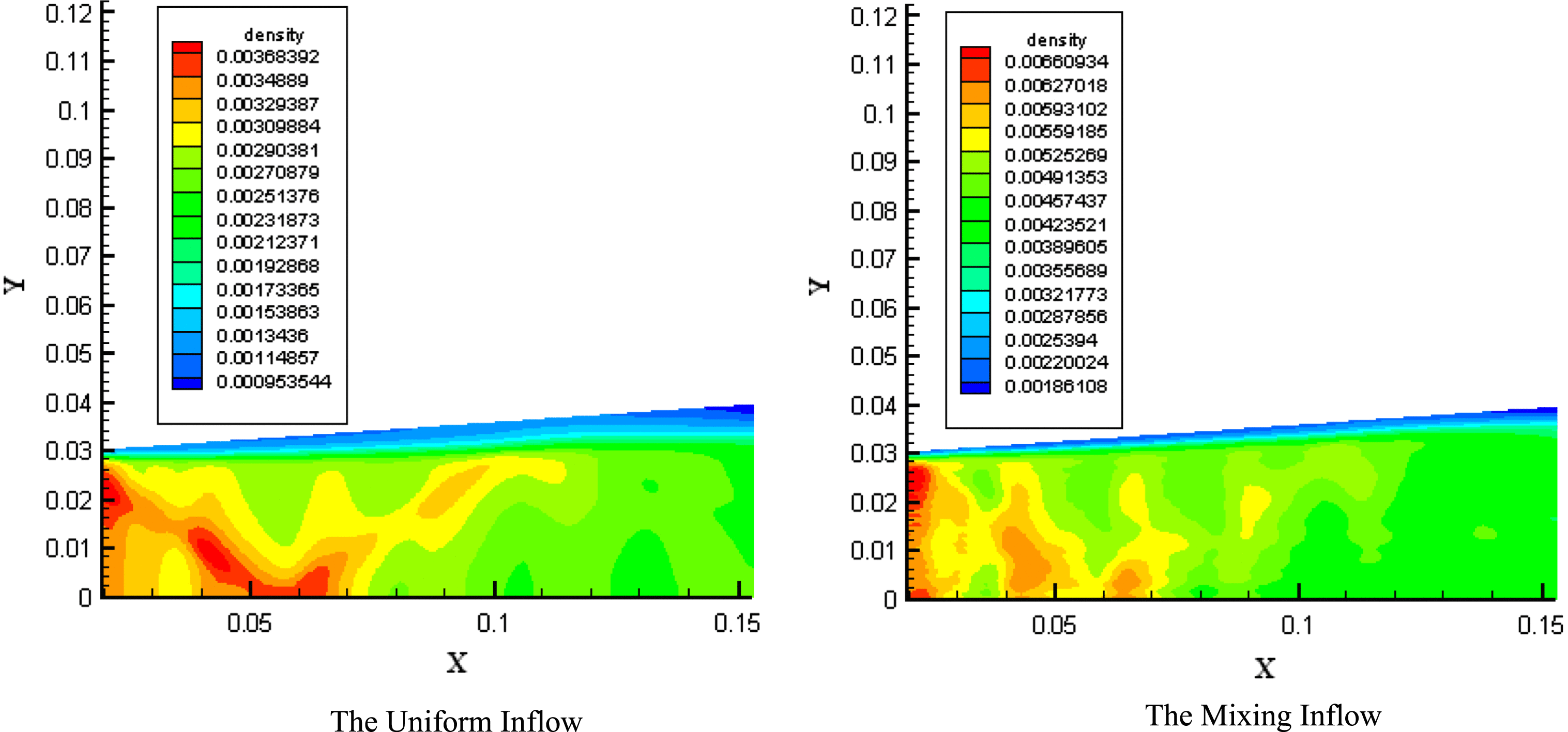
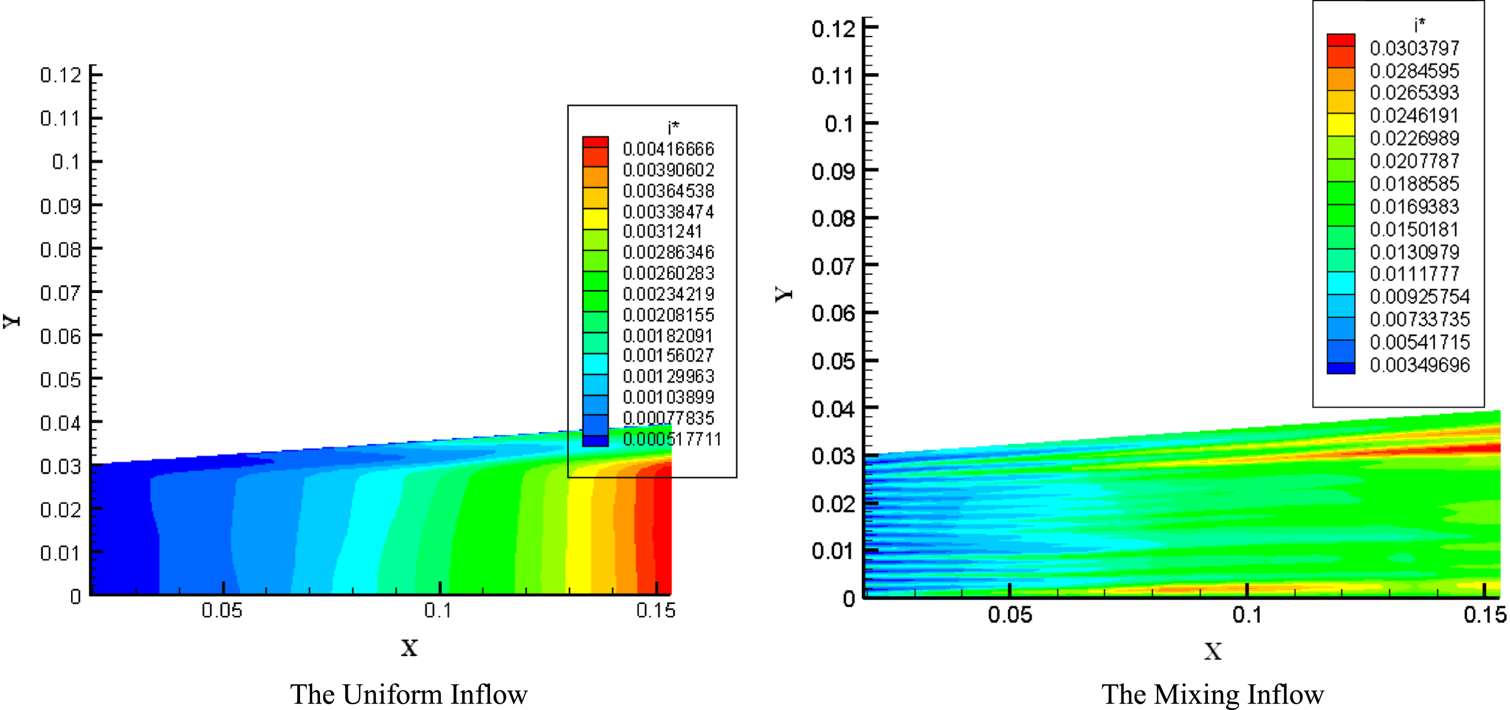
With the inflow boundary condition calculated according to the proposal in Section 2.4, the macroscale flow calculation is carried out over the resonator region with no lasing. And the steady-state flow field is obtained (see Figures 9 and 10). In order to evaluate the effect of the mixing inflow boundary condition on the cavity flow field, the results calculated with uniform inflow boundary condition are also shown in Figures 9 and 10.
It can be seen from Figure 9 that the mass density distributions are almost the same. The effects due to nozzle tail flow and boundary layer can be clearly observed, but the mixing influence is not obvious. However, Figure 10 shows significant differences in the excited atom iodine mass fraction distributions between the assumptions. Thus, the mixing influence should be considered in the lasing simulation.
Figure 9. The predicted density distributions at a plane normal to the optical axis.
Figure 10. The predicted excited atom iodine mass fraction distributions at a plane normal to the optical axis.
3.3. Lasing in the optical resonator
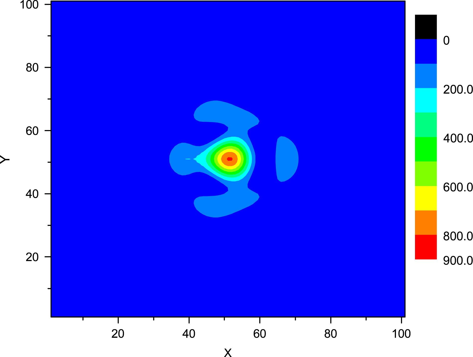
The laser power extraction characteristics are simulated in the entire resonator starting with the steady-state flow field obtained in the previous mixing inflow calculation. The flow and optical fields are simulated simultaneously as described in Section 2.5 until a steady state is achieved (see Figures 11–15). The far-field pattern is obviously a departure from the ideal diffraction-limited prediction (see Figure 12). The near-field intensity and phase profiles are not homogeneous. In the general case, the departure of the far-field pattern and phase inhomogeneities are the result of both gas density disturbances and variations in the individual constituent concentrations due to mixing and reaction. However, the inhomogeneities of the near-field intensity are also related to the gain medium flowing besides the inhomogeneities of gain medium. These pictures indicate that the inhomogeneities of gain medium is obtained and passed to the optical field in our calculation. The basic quantitative characteristic of an unstable resonator is the linear magnification  $M$ of the diameter of a light beam when it performs round trips from one mirror to the other. In other words, the laser mode cross section is different when the laser beam travels to different
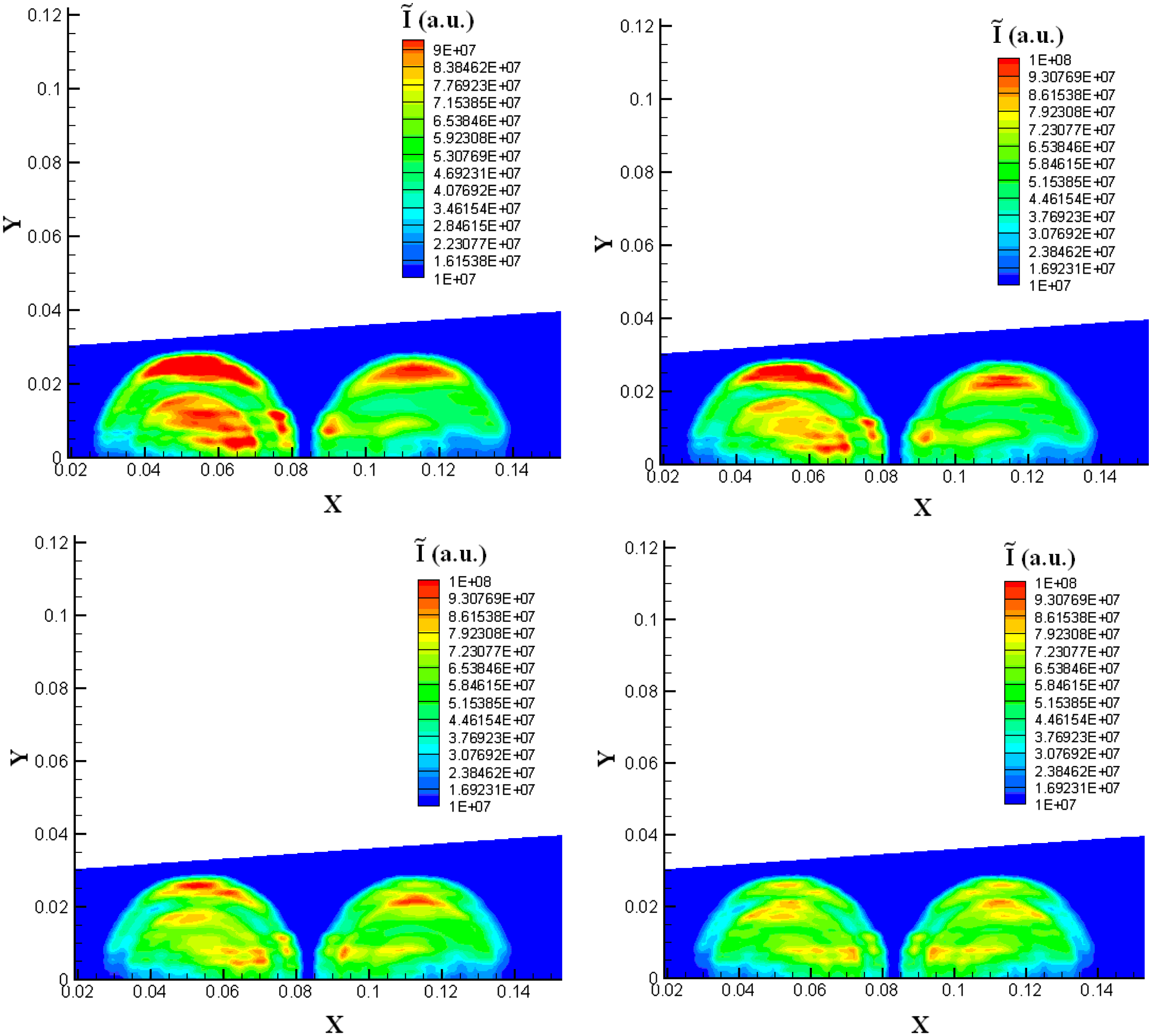
  $z$ stations. Therefore, the laser power extraction from the gain medium is different at different gain sheets. The difference of laser power extraction induces the difference of the flow field, and then further enhances the difference of near-field intensity profiles at different gain sheets (see Figure 13). These results indicate that further ‘gain sheet’ calculations are needed in order to simulate COIL lasing more accurately.
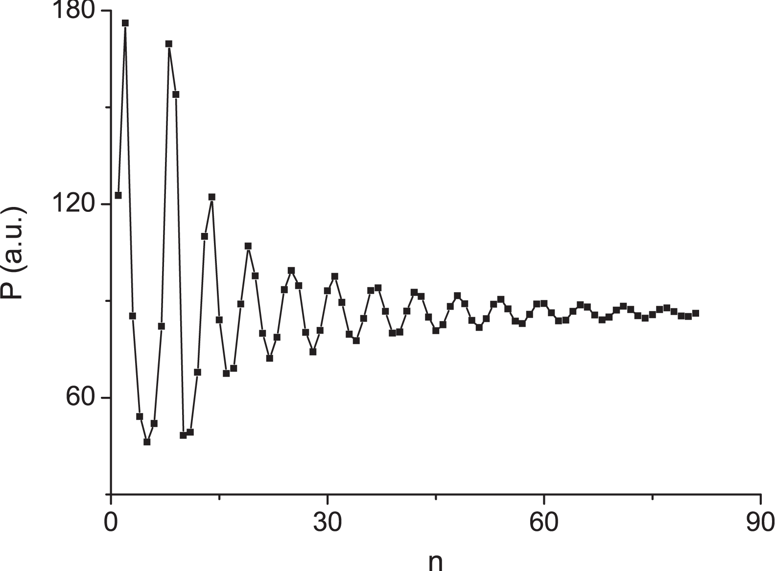
Figure 11. The predicted output power convergence history.
Figure 12. The far-field intensity profile (beam quality  $\beta = 1. 459275$).
Figure 13. Comparison of the near-field intensity profiles at different gain sheets with four gain sheet calculations.
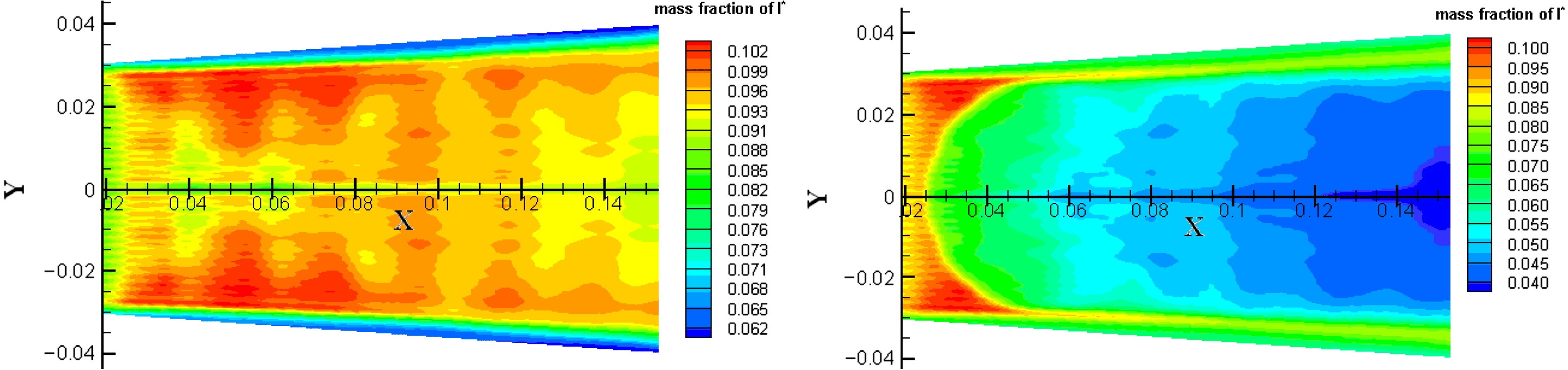
Figure 14 shows the predicted mass density profiles at a plane normal to the optical axis without lasing and with lasing. X-shaped and vertical arris patterns can be clearly observed in these profiles. The X-shaped shock pattern occurs from expansion/compression waves generated on the cavity top and bottom shrouds, and could be cancelled by the cavity wall contour design or operating conditions. The densities near the X-shaped patterns have higher values; these arise from compression and shock waves generated on the cavity top and bottom shrouds. The vertical arris patterns arise from nozzle tail flow. The flow at the exit of each nozzle is not exactly parallel; this is due to truncation of the nozzles to obtain structural strength at the tips and to the boundary layer growth along the nozzle walls as well as the wake growth downstream of the tips. The underexpanded flow stream exiting the nozzle goes through a Prandtl–Meyer expansion, and the flow is turned and accelerated. The multinozzle arrangement creates an interaction between the flow streams so that, when the accelerated flows meet, wake regions are created along with oblique shocks and recompression regions. Hence a diamond shock pattern is always a characteristic of such multinozzles (see Figure 15), and could not be combed out, but could be decreased by the nozzle contour design or operating conditions or putting the cavity downstream. The three-dimensional interaction of the diamond shock with the shock and expansion waves produces discrete high- and low-density regions, correlated with the X-shaped shock patterns visible in Figure 14. Figure 14 also shows no significant differences in mass density profiles without lasing and with lasing. However, careful observation reveals that the density distribution is disturbed slightly by heat release with lasing. The boundary layer growth is obvious along the cavity walls (see Figures 14 and 16). The large boundary layer thickness also tends to distort the flow near the nozzle exit and generates compression and shock waves.
During power extraction in the laser cavity, the circulating intensity rapidly builds and seeks whatever value is required to satisfy the round-trip loop-gain equal-loss condition for steady-state lasing. The iodine atom population inversion is rapidly depleted by stimulated emission and maintained at the threshold value. This is shown in Figure 16, where the cavity excited atom iodine mass fraction is seen to drop rapidly at the mirror leading edge. The nozzle exit plane is at the left-hand side of the figure and the abrupt decrease in the excited atom iodine mass fraction corresponds to the mirror location. Thus the  ${\mathrm{I} }^{\ast } $ pumping reaction is driven out of equilibrium and the ${\text{O} }_{2} \mathop{(}\nolimits ^{1} \hspace {-2.5pt} \mathrm{\Delta} )$ population is rapidly depleted by the forward rate. From the cavity the excited oxygen density is reduced to its threshold value, the gain goes to zero and no more power can be extracted. The gain, the excited atom iodine mass fraction and the ${\text{O} }_{2} \mathop{(}\nolimits ^{1} \hspace {-2.5pt} \mathrm{\Delta} )$ mass fraction are not disarranged in the region not interrogated by the optical mode.
Figure 14. Comparison of mass density profiles without/with lasing.
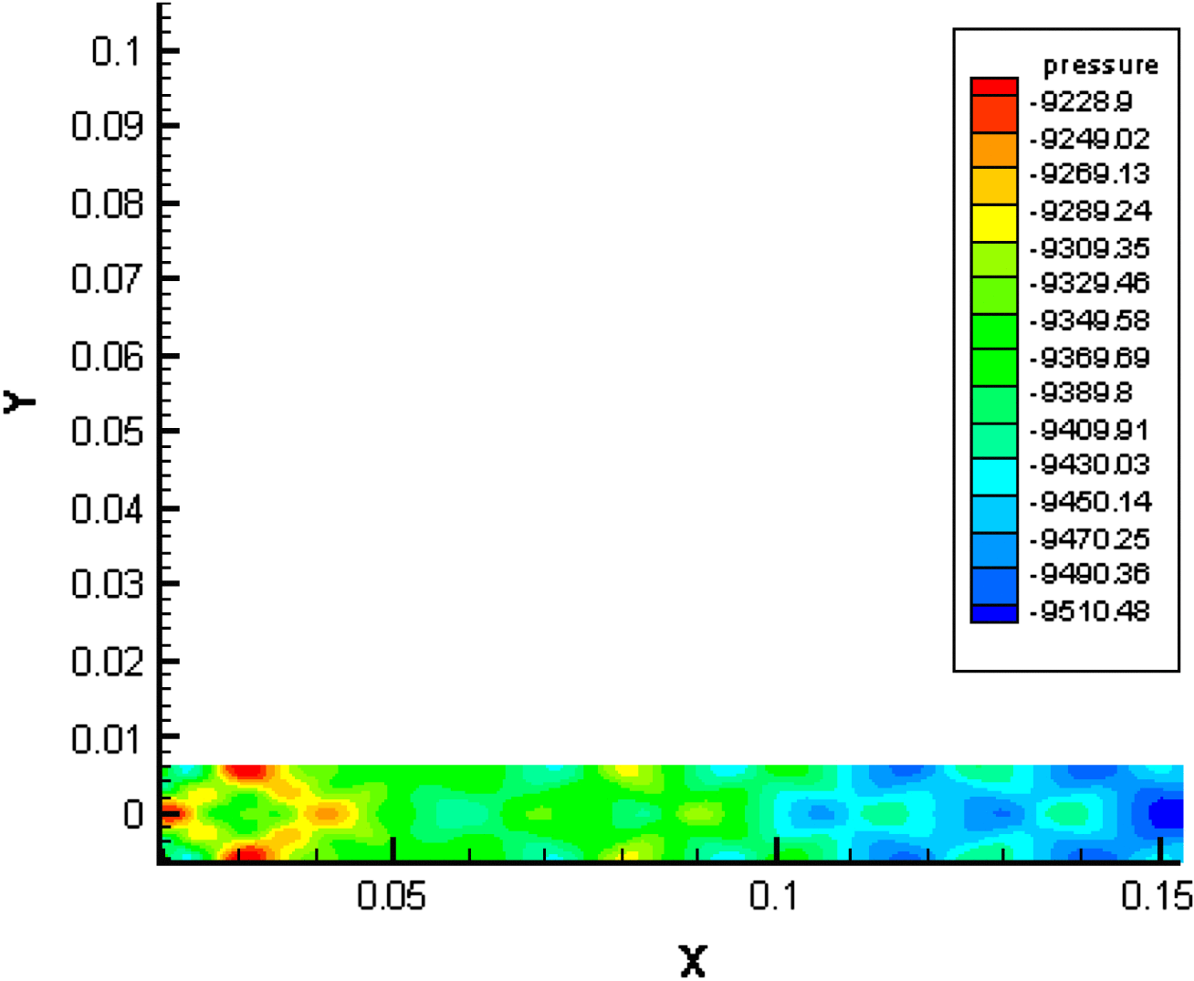
Figure 15. The predicted pressure distributions at a plane parallel to the optical axis.
Figure 16. Comparison of excited atom iodine mass fraction distributions without/with lasing.
4. Conclusions
The modeling of lasing in a chemical oxygen–iodine laser (COIL) medium is proposed, which is coupling with the effects induced by transverse injection of secondary gases, non-equilibrium chemical reactions, nozzle tail flow and boundary layer. The coupled steady solutions of the fluid dynamics and optics in a COIL complex three-dimensional cavity flow field are obtained following the proposal. A feasible methodology and a theoretical tool are offered to predict the beam quality for large-scale COIL devices.
The modeling results show that the effects have some influence on the lasing properties, which are induced by transverse injection of secondary gases, non-equilibrium chemical reactions, nozzle tail flow and boundary layer. There are obvious differences of near-field intensity profiles at different gain sheets. This result indicates that more ‘gain sheet’ calculations are needed in order to simulate COIL lasing more accurately. Or, in other words, the number of gain/intensity sheets should be selected to adequately resolve the intensity variations along the optical axis and is varied to verify insensitivity to the final beam quality result.
The communication architecture between fluid dynamics simulation and optics simulation has been developed via a file transfer protocol on an interim basis, as was done in[Reference Lampson, Plummer, Erkkila, Crowell and Helms8]. The ultimate objective is to perform both the fluid dynamics simulation and the optics simulation in one code. The mesh refinement studies will be done with the codes to see if the solution changes as the mesh size is reduced further and further.


 Open access