


1. Introduction
High-throughput high-dimensional marker platforms are now available for many species. The Affymetrix Genome-Wide Human SNP Array 6.0 (http://www.affymetrix.com) has been available for some time and has almost 1 million SNPs in a 1·8 million marker array. New generation sequencing techniques (Varshney et al., Reference Varshney, Nayak, May and Jackson2009) promise an explosion of data that will be challenging for association studies, quantitative trait locus (QTL) analysis and genomic prediction. There is a need to provide statistical methods that handle high-dimensional data. The focus of this paper is QTL analysis in plants, however, the methods presented could be applied to any species.
Estimated sizes of QTLs are often used by researchers to further their understanding of the impact of individual QTL. However, it has been understood for some time that QTL analysis leads to biased estimates of putative QTL effect sizes. Beavis (Reference Beavis1994, Reference Beavis and Patterson1998) discusses the inflated effects that result from QTL analyses, Xu (2003) provides a theoretical justification, while Melchinger et al. (Reference Melchinger, Utz and Schön1998) also conclude that sizes are inflated. Developing methods that reduce bias is desirable.
There are many methods available for the analysis of QTL; it is not possible to review all the methods so a selection of key papers are discussed. Initial methods of analysis used individual markers (Weller, Reference Weller1986) and interval mapping using mixture models (Lander & Botstein, Reference Lander and Botstein1989). Haley & Knott (Reference Haley and Knott1992) and Martinez & Curnow (Reference Martinez and Curnow1992) introduced the regression approach for interval mapping. The bias in simple interval mapping led to composite interval mapping (CIM; Zeng, Reference Zeng1994; Jansen, Reference Jansen1994) in which co-factors are used to control for other QTLs when searching for a single QTL. This, however, requires the selection of co-factors. Interval mapping and CIM usually involve fitting models at regular intervals along the genome and permutation for determining genome-wide thresholds for significance which can be very time-consuming. To overcome this latter problem, Piepho (Reference Piepho2001) presents a fast approximate method for determining the threshold for both interval mapping and CIM. Multiple interval mapping (MIM; Kao et al., Reference Kao, Zeng and Teasdale1999) was introduced to try and improve detection of QTL by allowing multiple rather than single QTL to be fitted at the same time. This approach requires some knowledge of how many QTLs are present and there are model selection issues. The aim of CIM and MIM is to allow for multiple QTLs in the analysis because the presence of other QTL impacts on the estimation of each QTL.
Bayesian methods have been used extensively in QTL analysis, in particular for mapping multiple QTLs (Satagopan et al., Reference Satagopan, Yandell, Newton and Osborn1996; Heath, Reference Heath1997; Sillanpää & Arjas, Reference Sillanpää and Arjas1998, Reference Sillanpää and Arjas1999; Xu, Reference Xu2003; Yi, Reference Yi, George and Allison2004; Wang et al., Reference Wang, Zhang, Li, Masinde, Mohan, Baylink and Xu2005); for an excellent review, see Yi & Shriner (Reference Yi and Shriner2008). Che & Xu (Reference Che and Xu2010) present a fast method for determining thresholds in a Markov chain Monte Carlo approach. There are methods (Xu, Reference Xu2003; Yi et al., Reference Yi2003) that incorporate all the markers simultaneously, thereby removing the need to select co-factors or the specific number of QTLs in MIM.
Verbyla et al. (Reference Verbyla2007) presented a non-Bayesian whole genome average interval mapping (WGAIM) approach for QTL analysis of a single trait in a single trial in which all the intervals on a linkage map are used simultaneously. While this adds some complexity, it overcomes the need for repeated genome scans and a threshold for QTL detection is readily available. In addition, because mixed models are used for analysis, non-genetic effects, such as terms for experimental design, are easily included. WGAIM uses forward selection hence the number of analyses are greatly reduced. A simple random effects working model is used in which all the intervals are allowed to contain a possible QTL and a likelihood ratio test of significance of the random effects working model is conducted to decide if selection of a putative QTL is warranted. If selection is warranted, a two-stage outlier procedure (firstly linkage groups then intervals within a selected linkage group) is used to select the most likely putative QTL, that is then moved to the fixed effects part of the model. The approach shown by Verbyla et al. (Reference Verbyla2007) was much more powerful than CIM, although there is a small increase in selecting false positives. The approach has been implemented in the R environment (R Development Core Team, 2012) in the package wgaim; see Taylor & Verbyla (Reference Taylor, Verbyla, Cavanagh and Newberry2011). Note that although the original formulation of WGAIM used intervals, the wgaim package also allows analysis using markers rather than intervals.
While WGAIM performs well, there are aspects of the approach that require refinement. Since WGAIM uses all the intervals (or markers) simultaneously, an efficient method of analysis is required when the number of intervals (or markers) is very large, typically much larger than the number of observations on the trait of interest. The (selection) bias of WGAIM was not examined by Verbyla et al. (Reference Verbyla2007). The outlier procedure uses two stages and this can influence the results. This paper addresses the high-dimensional problem, the issue of bias and the outlier procedure. The high-dimensionality question is addressed by reformulating the random effects model for QTL sizes in WGAIM in such a way that the size of a random term is equal to the number of lines with marker data when the number of markers is greater than the number of lines. The question of selection bias is addressed by assigning each putative QTL to a random effect, rather than moving them to the fixed effects component of the model, in the forward selection process. Thus, the resulting model has multiple random components, a separate component for each putative QTL and one component for non-QTL. This procedure is called RWGAIM in this paper. The other modification of WGAIM is the reduction of the outlier procedure from two stages, linkage groups then intervals, to a one-stage procedure based only on intervals. This is applicable to WGAIM, yielding a method called WGAIMI, and to RWGAIM.
The paper is organized as follows. Firstly, the WGAIM approach is outlined. The extension that allows for more markers than genetic lines on a trait is presented. Then a modification of WGAIM is described in which each putative QTL is placed in a random effect rather than a fixed effect as they are selected. Thirdly, an intuitive argument is used to justify using a single stage outlier procedure for selection of putative QTL. Three simulations are conducted to examine the three aspects. In the first, the number of markers was varied for a fixed number of lines to compare timings using a conventional and the dimension reduction approach for analysis. This simulation involves low to moderate numbers of markers to facilitate the comparison. The second simulation considers genuine high-dimensional situations, with both population sizes and marker numbers varying. Lastly, a simulation study using the setup along the lines of Verbyla et al. (Reference Verbyla2007) is used to assess the impact of using random effects for the QTL selected and the single stage outlier procedure using WGAIM, WGAIMI and RWGAIM. Detection of QTL, false positive rates and importantly the estimated sizes of QTL are summarized. A wheat-doubled haploid population is used to conduct a QTL analysis using WGAIM, WGAIMI and RWGAIM to provide a further comparison of results across the methods. The paper finishes with a brief discussion.
2. Methods
The general scheme and differences between the WGAIM, WGAIMI and RWGAIM approaches are outlined in Fig. 1 and are detailed below. Equation numbers in Fig. 1 refer to those in the text.

Fig. 1. Scheme for WGAIM, WGAIMI and RWGAIM. Difference between the approaches is indicated in italics and the equations in the text corresponding to each step are indicated in brackets where relevant.
(i) WGAIM
Verbyla et al. (Reference Verbyla2007) used mixed models as the basis for QTL analysis because the experiments to be analysed involved design effects and possibly other non-genetic effects that should be accounted for in the analysis. The models fitted to the data are of the form
 $${\bi y} \equals {\bi X\tau } \plus {\bi Z}_{\setnum{0}} {\bi u}_{\setnum{0}} \plus {\bi Z}_{g} {\bi u}_{g} \plus {\bi e}\comma $$
where the vector y (n × 1) consists of trait data. The components of (1) reflect the nature of the study. Thus, X (n×t) and Z0 (n×b) are known design matrices for fixed and random effects, respectively, that arise from the design of the study and non-genetic sources of variation (Smith et al., Reference Smith, Lim and Cullis2005, Reference Smith, Cullis and Thompson2006), τ is the vector of fixed effects parameters, and u0 is a vector of random effects. The vector of residual effects is denoted by e and this term and u0 are assumed independent, mean zero with variance–covariance matrices R and G0, respectively. The forms for R and G0 will reflect the nature of the analysis.
If there are ng lines of interest, the vector of genetic effects, ug, is ng × 1. The design matrix Zg in (1) assigns the appropriate genetic effect to each observation and thus consists of zeros and ones.
The WGAIM approach requires a baseline model to be fitted. This means specifying the genetic effects ug. The standard model is the so-called infinitesimal model or polygenic model for which
 $$\mathop {\bi u}\nolimits_{g} \equals {\bi u}_{p} \comma $$
where  ${\bi u}_{p} \sim N\lpar {\bf 0}\comma \sigma _{p}^{\setnum{2}} {\bi I}_{n_{g} } \rpar $; if pedigree information is available, more complex models can be fitted (Oakey et al., Reference Oakey, Verbyla, Pitchford, Cullis and Kuchel2006).
The next step in WGAIM is to include the interval (or marker) regression. This is called the working model in Verbyla et al. (Reference Verbyla2007). Firstly, note if there are c linkage groups (or chromosomes) with linkage group k having rk markers, hence we assume
 $${\bi u}_{g} \equals \mathop{\sum}\limits_{k \equals \setnum{1}}^{c} \,\mathop{\sum}\limits_{j \equals \setnum{1}}^{r_{k} \minus \setnum{1}} \,{\bi q}_{kj} a_{kj} \plus {\bi u}_{p} \comma $$
where qkj is a vector of scores for a potential QTL in interval j of linkage group k; akj is the corresponding size of the QTL. The QTL scores reflect the two possible genotypes, AA and BB for doubled haploid and recombinant inbred lines, and AB and BB for back-cross populations; the scores are 1 and −1 for the two genotypes. As qkj is unknown, by using the regression approach (Haley & Knott, Reference Haley and Knott1992; Martinez & Curnow, Reference Martinez and Curnow1992), it is replaced by its conditional expectation given flanking markers mkj and mk,j + 1. The expression is given in Verbyla et al. (Reference Verbyla2007) and involves θk ;j,j + 1, the recombination frequency between markers j and j + 1 on linkage group k, and θkj, the recombination fraction between marker j and the possible QTL in that interval. Verbyla et al. (Reference Verbyla2007) further average out the location by assuming the distance from the marker j to the QTL is uniformly distributed on the interval, thereby eliminating θkj. This results in the model
 $$\eqalign{ {\bi u}_{g} \equals \tab \mathop{\sum}\limits_{k \equals \setnum{1}}^{c} \,\mathop{\sum}\limits_{j \equals \setnum{1}}^{r_{k} \minus \setnum{1}} \,\lpar {\bi m}_{kj} \plus {\bi m}_{k\comma j \plus \setnum{1}} \rpar \; \psi _{kj} \; a_{kj} \plus {\bi u}_{p} \comma \cr \equals \tab {\bi M}_{E} {\bi a} \plus {\bi u}_{p} \comma \cr} $$
where ψkj = θk ;j,j + 1/2dk ;j,j + 1(1 − θk ;j,j + 1) and dk ;j,j + 1 is Haldane's distance between markers j and j + 1 on linkage group k. Note that ME is a known matrix of pseudo-markers spanning the whole genome. To complete the working model, it is assumed that a∼N(0,σa 2Ir−c) where  $r \equals \sum _{k \equals \setnum{1}}^{c} r_{k} $. This is a very simple model and aims to provide a mechanism for determining if a putative QTL can be selected.
The WGAIM process starts by fitting (1) with (2) and (1) with (4) and conducting a residual likelihood ratio test of the hypothesis H 0: σa 2 = 0. Under H 0, the statistic has a distribution that is a mixture of chi-squared distributions, namely 0·5χ02 + 0·5χ12 (Stram & Lee, Reference Stram and Lee1994). If the hypothesis is rejected, this suggests that there is at least one putative QTL.
To select the most likely interval for the putative QTL, an outlier detection approach is used. Verbyla et al. (Reference Verbyla2007) use the alternative outlier model (AOM). In the original formulation, the process occurred in two steps. Firstly, an outlier model was proposed at the level of the linkage group. Thus, the model proposed was
 $${\bi u}_{g} \equals {\bi M}_{E} \; \lpar {\bi a} \plus {\bi D}_{k} {\bimdelta }_{k} \rpar \plus {\bi u}_{p} \comma $$
where Dk is an (r−c) × (rk − 1) matrix with a one in position corresponding to each interval j on linkage group k and zero elsewhere. It is assumed  ${\bimdelta }_{k} \sim N\lpar 0\comma \sigma _{a\comma k}^{\setnum{2}} {\bi I}_{r_{k} \minus \setnum{1}} \rpar $. The idea behind this formulation is that if a putative QTL exists on linkage group k, the size of the effects of the putative QTL will be inflated by δk through an increase in variance. Although it appears that many models have to be fitted, in fact a procedure based on a score statistic for the hypothesis H 0: σa ,k2 = 0 was used by Verbyla et al. (Reference Verbyla2007), and this only relies on the fit of (1) with (4). The selection of the linkage group that contains the putative QTL is based on the outlier statistics given by
 $$t_{k}^{\setnum{2}} \equals {{\sum\nolimits_{j \equals \setnum{1}}^{r_{k} \minus \setnum{1}} \,\mathop {\tilde{a}}\nolimits_{kj}^{\setnum{2}} } \over {\sum\nolimits_{j \equals \setnum{1}}^{r_{k} \minus \setnum{1}} \,{\rm var\lpar }\mathop {\tilde{a}}\nolimits_{kj} {\rm \rpar }}}\comma $$
where  ${\tilde{a}}\nolimits_{kj} $ is the best linear unbiased predictor (BLUP) of the size akj of a QTL in interval j on linkage group k, and var (${\tilde{a}}\nolimits_{kj} $) is its variance. The linkage group with the largest statistic tk 2 is selected as containing the putative QTL. Once the linkage group is selected, the interval on that linkage group most likely to contain a putative QTL is selected. This involves a similar AOM, for intervals on linkage group k, namely
 $${\bi u}_{g} \equals {\bi M}_{E} \lpar {\bi a} \plus {\bi d}_{kj} \delta _{kj} \rpar \plus {\bi u}_{p} \comma $$
where dkj is a vector with a one in position corresponding to interval j on linkage group k and  $\delta _{kj} \sim N\lpar 0\comma \sigma _{a\comma kj}^{\setnum{2}} \rpar $. A score statistic for the hypothesis $H_{\setnum{0}} \colon \sigma _{a\comma kj}^{\setnum{2}} \equals 0$ is used again and the outlier statistic is
 $$t_{kj}^{\setnum{2}} \equals {{\mathop {\tilde{a}}\nolimits_{kj}^{\setnum{2}} } \over {{\rm var}\lpar \mathop {\tilde{a}}\nolimits_{kj} \rpar }}.$$
The interval with the largest tkj 2 is selected as containing the putative QTL. This QTL interval is moved to the fixed effects. The forward selection continues with (2) and (4) replaced by
 $${\bi u}_{g} \equals {\bi m}_{E\comma \setnum{1}} a_{\setnum{1}} \plus {\bi u}_{p} \comma $$
 $${\bi u}_{g} \equals {\bi m}_{E\comma \setnum{1}} a_{\setnum{1}} \plus {\bi M}_{E\comma \minus \setnum{1}} {\bi a}_{ \minus \setnum{1}} \plus {\bi u}_{p} \comma $$
where mE,1 is the vector of pseudo-marker scores for the first putative QTL and a 1 is the size of that QTL. ME, − 1 is the matrix of scores for those pseudo-markers that have not been selected as putative QTL and a−1 is the vector of effect sizes for those pseudo-markers.
The process is repeated. Thus both (1) with (7) and (1) with (8) are fitted and the likelihood ratio test for H 0: σa 2 = 0 is carried out again. If H 0 is rejected, another putative QTL is selected using the approach based on the AOM. After s such selections the working model (4) has become
 $${\bi u}_{g} \equals \mathop{\sum}\limits_{l \equals \setnum{1}}^{s} \,{\bi m}_{E\comma l} a_{l} \plus {\bi M}_{E\comma \minus s} {\bi a}_{ \minus s} \plus {\bi u}_{p} \comma $$
so that we have two terms involving the pseudo-marker effects. The first term involves the putative QTL; al is the size of the lth QTL and mE,l are the corresponding pseudo-marker scores for the interval defining l. The second term contains the interval that has not been selected so that a−s is the vector of sizes of QTL that may yet be chosen (most of them will not be selected) with corresponding scores ME, − s. After all putative QTL have been selected, the QTL are summarized by listing the putative QTL, the size of QTL found, and a P-value indicating the level of significance for each putative interval.
(ii) High-dimensional analysis
A major issue concerns the possible high dimension of ME in (4) or of ME, − s in (9) at stage s of selection. For ease of presentation, we consider the first step of selection. The matrix ME is of size ng×r−c, and r−c may be very large, larger than ng. If ng>r−c there is no need to invoke dimension reduction. If ng<r−c, it is possible to carry out efficient computations not in dimension r−c, but in dimension ng which may be much smaller, and subsequently recover the r−c effects necessary for selection.
Our approach is similar to that proposed by Stranden & Garrick (Reference Stranden and Garrick2009) in the context of genomic selection. For generality, suppose that a∼N(0,σa 2Ga). In WGAIM, Ga=Ir−c. Taylor et al. (Reference Taylor, Diffey, Verbyla and Cullis2012) consider an alternative approach based on penalized likelihoods and in that case at stage k of the iterative process involved, Ga=Wk where Wk is a diagonal matrix of known weights. In these cases, Ga is a known matrix and the results of this section will hold for any method in which this is the case or can be constructed to be so. Note that while WGAIM involved pseudo-markers for intervals, these can be replaced by marker scores (and would be in the genomic prediction situation).
Thus, suppose for the moment that no putative QTLs have been selected (s = 0 in the discussion above). The variance model for the random effects MEa is of the form
 $$\sigma _{a}^{\setnum{2}} {\bi M}_{E} {\bi G}_{a} {\bi M}_{E}^{T} \comma $$
which is of size ng×ng. The matrix MEGaMET is known. Then, we can re-formulate the working mixed model (4) as follows. Let
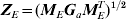 $${\bi Z}_{E} \equals \lpar {\bi M}_{E} {\bi G}_{a} {\bi M}_{E}^{T} \rpar ^{\setnum{1}\sol \setnum{2}} $$
denote the matrix square root; this can be found by using the singular value decomposition (Golub & van Loan, Reference Golub and van Loan1996). If we define an ng × 1 vector a* as
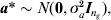 $${\bi a\ast } \sim N\lpar {\bf 0}\comma \sigma _{a}^{\setnum{2}} {\bi I}_{n_{g} } \rpar \comma $$
the working model term for interval effects MEa can be replaced by
 $${\bi Z}_{E} {\bi a\ast }$$
and the same variance model (10) is obtained. Thus, we can estimate ng effects rather than r−c.
Most importantly for QTL analysis, however, the r−c effects can be recovered. Note firstly that the BLUP for a* is given by
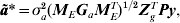 $${\bi \tilde{a}\ast } \equals \sigma _{a}^{\setnum{2}} \lpar {\bi M}_{E} {\bi G}_{a} {\bi M}_{E}^{T} \rpar ^{\setnum{1}\sol \setnum{2}} {\bi Z}_{g}^{T} {\bi Py\comma }$$
where P=H−1−H−1X(XTH−1X)−1XTH−1 and H=R+ZoGoZoT + σg 2ZgZgT + σa 2ZgMEGaMETZgT. The BLUP of a is given by
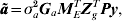 $${\bi \tilde{a}} \equals \sigma _{a}^{\setnum{2}} {\bi G}_{a} {\bi M}_{E}^{T} {\bi Z}_{g}^{T} {\bi Py}\comma $$
so that we can write
 $${\bi \tilde{a}} \equals {\bi G}_{a} {\bi M}_{E}^{T} \lpar {\bi M}_{E} {\bi G}_{a} {\bi M}_{E}^{T} \rpar ^{ \minus \setnum{1}\sol \setnum{2}} {\bi \tilde{a}}\ast \comma $$
thereby recovering the estimated size of potential QTLs in each interval from an analysis using the modified model.
To calculate the outlier statistics given by (5) and (6), we need the variance of  ${\bi \tilde{a}}$. This can be found using
 $$\eqalign{{\rm var\lpar }{\bi \tilde{a}}{\rm \rpar } \equals \tab {\bi G}_{a} {\bi M}_{E}^{T} \lpar {\bi M}_{E} {\bi G}_{a} {\bi M}_{E}^{T} \rpar ^{ \minus \setnum{1}\sol \setnum{2}} \hskip2pt{\rm var\lpar }{\bi \tilde{a}}\ast {\rm \rpar }\cr \tab \times \lpar {\bi M}_{E} {\bi G}_{a} {\bi M}_{E}^{T} \rpar ^{ \minus \setnum{1}\sol \setnum{2}} {\bi M}_{E} {\bi G}_{a}} $$
and so the variance matrix of the BLUPs of a* is required, that is  ${\rm var\lpar }{\bi \tilde{a}}\ast {\rm \rpar }$, again a lower-dimensional calculation after fitting the reduced dimensional model. Only the diagonal elements of ${\rm var\lpar }{\bi \tilde{a}}{\rm \rpar }$ are required together with (11) to calculate the outlier statistics (5) and (6). The full matrix need not be calculated in practice.
(iii) Random WGAIM
The details presented in Verbyla et al. (Reference Verbyla2007) differ in only one aspect for a random version of WGAIM (RWGAIM). In WGAIM (Verbyla et al. Reference Verbyla2007) the unselected effects are random effects (the working model in that paper) such that in (9), a−s∼N(0, σa 2I) and the selected effects as are fixed effects. The proposal for RWGAIM, is to assume  $a_{l} \sim N\lpar 0\comma \sigma _{al}^{\setnum{2}} \rpar $, so that the sizes are random effects, have their own variance (resulting in a random regression on the pseudo-marker scores mE,l) and all have a different variance to the unselected effects. This makes sense as putative QTL effects exhibit variation from zero because they are QTL. Thus, putative QTL are assumed to come from their own distribution and non-QTL come from another distribution. The distributions differ in their variances and not their means. This approach has the flavour of hierarchical models proposed by Griffin & Brown (Reference Griffin and Brown2010) and others in high-dimensional variable selection.
(iv) QTL selection using interval statistics only
In Verbyla et al. (Reference Verbyla2007) and as outlined above, the selection of a QTL takes place in two stages, with both stages using outlier statistics. In the first stage, an outlier statistic was calculated for each linkage group using (5), and the linkage group with the largest statistic was selected as containing a putative QTL. In the second stage, the interval with the largest outlier statistic on the selected linkage group was selected as containing the putative QTL using (6). This process works effectively in many situations. However, the size of the linkage group has an impact on the size of the outlier statistic in the first stage. This can be seen from (5). On small linkage groups, the size of effects relative to their variance will be larger than for large linkage groups. This is because while there will generally be a small number of large sizes where a putative QTL is present, the variances will generally be of comparable size across the whole linkage group. Thus, using the outlier statistic for linkage groups favours the selection of small linkage groups at the first stage. This problem is overcome if selection is based only on the outlier statistics for the intervals, that is (6), and the first stage is omitted. This is the approach adopted in WGAIMI and RWGAIM.
(v) Significance of QTL
Once all putative QTLs have been selected, they each constitute a random effect term. The size of the QTL effect is then a BLUP. It is no longer appropriate to test the hypothesis that the effect is zero in order to assess the significance of the putative QTL. Tests of hypotheses pertain to unknown parameters, and random effects involve distributions of effects.
To provide a measure of the strength of a QTL, the conditional distribution of the true (random) QTL effect al say, given the data are used. That is, under the normality assumptions for a linear mixed model,
 $$a_{l} \vert {\bi y}_{\setnum{2}} \sim N\lpar \mathop {\tilde{a}}\nolimits_{l} \comma \sigma _{{\rm PEV}\comma l}^{\setnum{2}} \rpar \comma $$
where y2 is the component of the data free of fixed effects (Verbyla, Reference Verbyla, Cullis and Thompson1990). The mean of this conditional distribution is the BLUP of al, that is the estimated size of the QTL ãl, and the variance is the prediction error variance (PEV) of al. Thus, the proper assessment of the impact of the QTL involves determining how far ãl is from zero relative to the variation as measured by σPEV,l. Clearly, distributions for which the mean is far from zero relative to the variation indicate a strong QTL effect, whereas distributions for which the mean is close to zero will indicate a weaker QTL.
To quantify this measure of strength of each putative QTL, it is possible to calculate a probability somewhat like a P-value, for which values close to 0 indicate that the QTL is strong. Consider the statistic
 $$X_{l}^{\setnum{2}} \equals \mathop {\left( {{{a_{l} \minus \mathop {\tilde{a}}\nolimits_{l} } \over {\sigma _{{\rm PEV}\comma l} }}} \right)}\nolimits^{\setnum{2}} \comma $$
which has a chi-squared distribution on 1 degree of freedom. Zero on the original scale is cl 2 = ãl 2 / σPEV,l2 on the chi-squared scale and so
 $${\rm Pr}\lpar X_{l}^{\setnum{2}} \gt c_{l}^{\setnum{2}} \rpar $$
provides a measure of the strength of the putative QTL through how far ãl is from zero relative to σPEV,l. In RWGAIM, this probability can be used to indicate the strength of the putative QTL.
Note also that while LOD scores are not necessary for WGAIM or RWGAIM (because the multiple testing problem is largely avoided), a LOD score for RWGAIM is given by
 $${\rm LOD}_{l} \equals {1 \over 2}\rm log_{\setnum{10}} \left( {{\rm e}^{c_{l}^{\setnum{2}} } } \right).$$
Lastly, the percentage of genetic variance accounted for by each putative QTL is of interest. This can be determined approximately for both WGAIM and RWGAIM as follows.
The genetic effects are specified by (9); once all putative QTL have been found s is the number of QTLs. If ql is the vector of QTL scores (−1 or 1) for QTL l, to facilitate an expression for the variance, we use a combination of (3) and (9) namely,
 $${\bi u}_{g} \equals \mathop{\sum}\limits_{l \equals \setnum{1}}^{s} \,{\bi q}_{l} a_{l} \plus {\bi M}_{E\comma \minus s} {\bi a}_{ \minus s} \plus {\bi u}_{p} .$$
Consider a single line i. The variance of the genetic effect for line i, ugi, is then given by
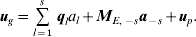
 $$\eqalign{ {\rm var}\left( {u_{gi} } \right) \equals \tab \left\{ {\sum\limits_{l \equals \setnum{1}}^{s} a_{l}^{\setnum{2}} \plus \mathop {\sum \sum }\limits_{l \ne l \prime} \lpar 1 \minus 2\theta _{ll \prime} \rpar a_{l} a_{l \prime} } \right\} \cr \tab \plus \sigma _{a}^{\setnum{2}} {\bi m}_{Ei\comma \minus s}^{T} {\bi m}_{Ei\comma \minus s} \plus \sigma _{p}^{\setnum{2}} \comma \cr} $$
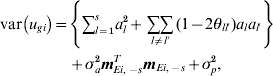
where we have allowed for linked QTL, θll ′ is the recombination fraction for QTL l and l′, and mEi,˗sT is the ith row of ME,−s. Thus, each line has its own (different) variance. To obtain an approximate measure of the total genetic variance, we define an ‘average’ line effect, ug*, by averaging the multiplier of σa 2 over lines. Thus, if
 $$m_{E\comma \minus ss} \equals {{\sum\nolimits_{i \equals \setnum{1}}^{n_{g} } {\bi m}_{Ei\comma \minus s}^{T} {\bi m}_{Ei\comma \minus s} } \over {n_{g} }}\comma $$
the variance of the ‘average’ line effect is taken as
 $${\rm var}\left( {u_{g}^{ \ast } } \right) \equals \mathop{\sum}\limits_{l \equals \setnum{1}}^{s} \,a_{l}^{\setnum{2}} \plus \mathop {\sum \sum }\limits_{l \ne l \prime} \,\lpar 1 \minus 2\theta _{ll \prime} \rpar a_{l} a_{l \prime} \plus \sigma _{al}^{\setnum{2}} m_{E\comma \minus ss} \plus \sigma _{p}^{\setnum{2}} .$$
Equation (14) specifies the approximate total genetic variance. A difficulty with using (14) to find percentage of variance is that the individual contributions of QTL can add up to more than 100% because of the covariance of linked QTL in repulsion. Given that the calculation is not precise, the covariances are ignored in the calculation so that
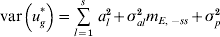 $${\rm var}\left( {u_{g}^{ \ast } } \right) \equals \mathop{\sum}\limits_{l \equals \setnum{1}}^{s} \,a_{l}^{\setnum{2}} \plus \sigma _{al}^{\setnum{2}} m_{E\comma \minus ss} \plus \sigma _{p}^{\setnum{2}} $$
is used for the total variance. Using (15), the percentage variance attributed to the lth QTL is then
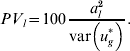 $$PV_{l} \equals 100{{a_{l}^{\setnum{2}} } \over {{\rm var}\left( {u_{g}^{ \ast } } \right)}}.$$
To calculate these values, al and other unknown parameters are replaced in (15) and (16) by their estimates from either the WGAIM or RWGAIM approach.
(vi) Computation
Both the high-dimensional approach and the RWGAIM approach have been implemented in the R environment (R Development Core Team, 2012) in the package wgaim (Taylor et al., Reference Taylor and Verbyla2011) which is available on CRAN (http://cran.r-project.org). This package requires the asreml (Butler et al., Reference Butler, Cullis, Gilmour and Gogel2011) and qtl (Broman et al., Reference Broman, Wu, Sen and Churchill2003, Reference Broman, Wu, Churchill, Sen, Arends, Jansen, Prins and Yandell2012) packages in R. In particular, it is the power of asreml that allows the complex models to be fitted. The wgaim package includes diagnostic plots and linkage map plots that allow the QTL to be displayed.
3. Materials
(i) Simulation studies
Three simulation studies were conducted.
(a) Comparison of conventional and dimension reduction analysis
To demonstrate the impact of the dimension reduction approach, a small simulation study was carried out. The population size was ng = 200 lines with two replicates. The phenotypic data were generated using the model (i = 1, 2, …, ng, k = 1, 2)
 $$y_{ik} \equals \mu \plus \sum\limits_{l \equals \setnum{1}}^{n_{q} } \,q_{il} a_{l} \plus u_{pi} \plus e_{ik} \comma $$
where the mean μ was 10, the polygenic effects upi are assumed N(0, 0·5) and eik were assumed independent and identically distributed N(0, 1). There were nq = 5 QTLs, with qil in (17) having a simulated allelic value (−1 or 1) for line i for QTL l. The size of this QTL is al and this is 0·5 for all QTLs. Thus, the mean line heritability (allowing for the two replicates) is approximately 0·85. The aim of having such a high heritability was to ensure that all 5 QTL would be detected to enable the timings to be compared.
The genetic data consisted of 10 linkage groups with the number of markers per linkage group varying from 21 to 101 in steps of ten markers; this allows the impact to be gauged from the case where the number of lines is close to the number of markers (210) to the case where the number of markers (1010) greatly exceeds the number of lines. Each linkage group was 250 cM long so that the density of markers changed from 12·5 cM intervals to 2·5 cM intervals. The five QTL were placed in the middle of each of five linkage groups. The bi-allelic marker scores were generated for each of the 200 lines for each scenario and the linkage map was then estimated as it would be in practice.
Two methods of analysis were carried out using RWGAIM using the one-stage outlier approach. One involved using the dimension reduction approach, while the other used the original method that involves using all the intervals explicitly. The aim was to provide a comparison of the time taken for each scenario using each of the methods.
(b) High-dimensional simulation study
To examine the effectiveness of the dimension reduction approach in genuinely high-dimensional situations, a second simulation was conducted. Using the same model as the first simulation, data were generated for population sizes 500, 1000 and 2000 lines in combination with 10 010, 20 010 and 50 010 markers (10 linkage groups with 101, 201 and 501 markers respectively) with QTLs at markers in the middle of 5 of the 10 linkage groups. As given above the linkage groups were 250 cm in length so that the density of the markers changed from 2·5 to 0·5 cM. The analysis of the generated data used markers rather than intervals. The computer processor timings of the analysis for each simulation from the nine combinations (population size by marker number) were determined.
(c) Power, false discovery rate and bias
The third simulation is similar to that conducted by Verbyla et al. (Reference Verbyla2007). The aim is to investigate three methods of QTL analysis, namely the original WGAIM approach using the two-stage outlier procedure, WGAIM using a one-stage outlier procedure (WGAIMI) and RWGAIM using a one-stage outlier procedure. These methods are expected to give similar results for QTL analysis apart from two key areas, short linkage groups and bias in estimated QTL sizes.
Nine linkage groups were simulated. On all linkage groups the markers were spaced at 10 cM. Linkage groups 5 and 9 had only two markers while the remaining linkage groups had 11 markers. Seven QTL (nq = 7) were placed at the midpoints of C1·4 (linkage group 1, interval 4), C1·8, C2·4, C2·8, C3·6, C4·4 and C5·1 as in Verbyla et al. (Reference Verbyla2007). C1·4 and C1·8 were in repulsion while C2·4 and C2·8 were in coupling; these QTL are 40 cM apart. Population sizes were 100, 200 and 400 lines each with two replicates.
Introducing two very short linkage groups was aimed at investigating the impact of the two-stage outlier procedure using linkage groups and the intervals as opposed to using a single-stage outlier procedure based on the intervals. This highlights the impact in an extreme situation.
Five hundred (500) simulations were carried out for each population size using (17) with al = 0·378, apart from C1·8 for which al = − 0·378. The polygenic effect had variance 0·5 and the residual variance was 1. The mean line heritability (allowing for the two replicates) is therefore 0·5.
For each population size, the three methods of analysis were carried out for each simulated dataset. Three sets of summaries were calculated for each method of QTL selection for each set of 500 simulations, namely
1. the proportion of correct detection of each QTL, including proportions for the QTL in coupling and repulsion,
2. the proportion of false positives, both linked (on the same chromosome as actual QTL) and unlinked (on chromosomes not containing QTL), and
3. means of estimated sizes of QTL effects for simulations where the QTL was selected. Empirical mean square error of prediction of the estimates were also found using all 500 simulations (not just those simulations where a true QTL was found).
As in Verbyla et al. (Reference Verbyla2007), a QTL was considered detected, if the correct interval or intervals on either side were selected.
(ii) Salinity trial
To illustrate the use of the random version of WGAIM, we analysed data from the experiment presented in Genc et al. (Reference Genc, Oldach, Verbyla, Lott, Hassan, Tester, Wallwork and McDonald2010). The aim of the experiment was to examine QTL for various traits under a salinity treatment and a non-saline environment in a hydroponic experiment.
A doubled-haploid bread wheat population (Berkut × Krichauff) was grown in supported hydroponics to identify QTLs associated with salinity tolerance traits. The experiment consisted of two runs in a growth cabinet. In each run, there were four trolleys on each side of the growth cabinet (blocks), each controlling two tubs. Each tub consisted of 9 rows and 5 columns with 3 positions being allocated to the input and output of the supported hydroponics and hence not having a line assigned. In each replication, the 152 DH lines were randomly allocated across two trolleys (and hence four tubs) with the two parents (Berkut and Krichauff) and two other standard lines (Baart and Kharchia) being also randomly allocated to each tub; thus, there were four replicates of each of the DH lines. Some traits were only measured on the saline treatment including shoot magnesium concentration (in parts per million per kg of dry matter) which is the trait analysed in this paper. Saline conditions tend to decrease magnesium concentration and searching for QTL that mitigate this effect is of interest. We only consider the first run because analysing two runs potentially involves a multi-environment QTL analysis which is beyond the scope of this paper.
Genotyping using 216 SSR markers was carried out using standard PCR conditions and subsequent gel electrophoretic separation on 8% polyacrylamide gels. In addition to the 216 SSRs and Vrn genes, 311 DArT markers were scored by Triticarte Pty. Ltd (http://www.triticarte.com.au). The linkage map was constructed using Map Manager QTX version QTXb20 (Manly et al., Reference Manly, Cudmore and Meer2001). Marker order was verified using RECORD (Van Os et al., Reference Van Os, Stam, Visser and Van Eck2005). Segregation ratios of two genotype classes (Berkut allele and Krichauff allele) at each locus were tested and markers deviating significantly from the expected ratio of 1:1 were excluded from QTL analysis. Re-estimation of genetic distance was performed using the Lander & Green (Reference Lander and Green1987) algorithm in the R (R Development Core Team, 2012) package qtl (Broman et al., Reference Broman, Wu, Churchill, Sen, Arends, Jansen, Prins and Yandell2012). Coincident markers were removed resulting in 379 distinct markers on 23 linkage groups for QTL analysis. The total length of the map was 3770 cM with an average spacing of 10·6 cM between the markers.
4. Results
(i) Simulation study: comparison of two methods of analysis
The simulations were conducted on a 64 Bit PC using Windows 7, with an Intel® Core™ i7-2860QM CPU at 2·50 GHz, with 16 Gb RAM at 2·39 GHz. The two methods of analysis are identical apart from dimension reduction and hence both methods resulted in the same five putative QTL as they should.
Figure 2 presents the CPU time required for each analysis from 210 to 1010 markers for the two methods of analysis. The dimension reduction approach resulted in times represented by the solid line, while the original method using all the markers explicitly resulted in the timings given by the broken line. The dimension reduction approach resulted in times that remained generally constant despite an increasing number of markers compared with the original approach where times increased exponentially. These trends for the two approaches would be expected to continue should the number of markers increase causing the original formulation to quickly become prohibitive, while the dimension reduction approach is expected to be able to deal with considerably large datasets.

Fig. 2. Computation time (in minutes) for analysis using the dimension reduction approach (solid line) and the approach using markers explicitly (broken line) for numbers of markers from 210 to 1010.
(ii) Simulation study: high-dimensional analysis
The dimension reduction approach was used for high-dimensional situations (10 010, 20 010 and 50 010 markers) for 500, 1000 and 2000 lines. In all the cases, 2000 lines were used in generation of marker data. Then, a random sample of lines was taken to obtain the data for 500 and 1000 lines for the simulations. Table 1 details the results in terms of the actual number of non-redundant markers and the computer processor time used in the analyses. The markers will be redundant because of very low recombination fractions and limited number of lines. Thus, for 500 lines, it was very difficult to retain large numbers of markers, with improvement as the number of lines increased. Note that with five QTLs, there are six steps in the forward selection process. Hence the time required per step can be calculated. This provides a base time line to gauge how long an analysis with a particular number of QTLs is likely to take. This is included in Table 1.
Table 1. High-dimensional simulations for varying population sizes and number of markers. Non-redundant markers varied with population size. Both the processor time and processor time per step of the forward selection process are presented

Firstly, note that for population sizes 500 and 1000 the analyses for the simulated data for all marker sizes were conducted using markers rather than intervals on the 64 bit PC outlined in the previous simulation. For population size 2000, the simulations were run on a high-performance computer requesting 16 Gb of memory. Only a single node was used.
For population size 500, the number of redundant markers restricted the size of the problem that could be investigated. The number of non-redundant markers increases with population size and subsequently the processor time goes up by a factor of 9-fold for each step as we move from 500 to 1000 to 2000. Thus, for 2000 lines and approximately 30 000 markers, the analysis took about 6 h.
The conclusion from this simulation study is that QTL analysis can be performed even for very high-dimensional data, possibly using high-performance computing facilities. The limitations are memory and storage usage in the R environment and the ability of the asreml software to handle such large dense datasets. These aspects increase the required time for analysis of very high dimensions.
(iii) Simulation study: power, false discovery rate and bias
The results of the simulations with seven QTLs as described above are presented in Tables 2–6. Each aspect is now discussed in turn.
Table 2 presents the proportion of simulations in which each QTL was successfully found using the original WGAIM (applying the two-stage outlier procedure), WGAIMI (applying the one-stage outlier procedure) and RWGAIM (applying the one-stage outlier procedure). The results are very similar for all three methods although WGAIM finds marginally more QTLs in total for all population sizes. This is mainly because original WGAIM tends to find the QTL at C5·1 more often than the other methods; this is a linkage group with only one interval. The WGAIM approach also tends to find more of the QTL in repulsion (C1·4 and C1·8) than the other two methods but less QTLs in coupling (C2·4 and C2·8) than RWGAIM. Apart from C5·1, however, it is RWGAIM that finds more QTLs although the differences are small. All three methods perform very well. Approximate standard errors can be found using the standard results for binomial proportion and are indicated in all the tables. These standard errors provide an idea of the scale of differences between methods. For example, the difference between the three methods for the QTL at C5·1 is clearly highly significant.
Table 2. Proportion of 500 simulations in which the QTL was detected for WGAIM, WGAIMI and random WGAIM (RWGAIM) analyses. The standard error for a proportion can be based on binomial distribution, that is  $\sqrt {\hat{p}\lpar 1 \minus \hat{p}\rpar \sol 500} $. For $\hat{p} \equals 0{\cdot}1$ (and hence $\hat{p} \equals 0{\cdot}9$), the standard error is 0·013, for $\hat{p} \equals 0.3$ the standard error is 0·020 and for $\hat{p} \equals 0.5$ the standard error is 0·022

Two-way tables for the proportions of QTLs detected for the two QTLs in repulsion are given in Table 3. Results for WGAIM, WGAIMI and RWGAIM are generally very similar, though the WGAIM method detects both QTLs more often than the other methods for all population sizes. For the two QTLs in coupling, the corresponding results are given in Table 4. Although the detection rates compared with repulsion were lower, RWGAIM shows a small improvement over WGAIM and WGAIMI in detecting both QTLs.
Table 3. Two way tables for the QTL in repulsion (C1·4 and C1·8) with proportions of the 500 simulations for each population size for the combinations of non-detected  $\overline{D}$ and detected D QTL. C1·4 is on the left and C1·8 on the top of each 2 × 2 table. The standard error for a proportion can be based on binomial distribution, that is $\sqrt {\hat{p}\lpar 1 \minus \hat{p}\rpar \sol 500} $. For $\hat{p} \equals 0{\cdot}1$ (and hence $\hat{p} \equals 0{\cdot}9$) the standard error is 0·013, for $\hat{p} \equals 0{\cdot}3$ the standard error is 0·020 and for $\hat{p} \equals 0{\cdot}5$ the standard error is 0·022

Table 4. Two way tables for the QTL in coupling (C2·4 and C2·8) with proportions of 500 simulations for each population size for the combinations of non-detected $\overline{D}$ and detected D QTL. C2·4 is on the left and C2·8 on the top of each 2 × 2 table. The standard error for a proportion can be based on binomial distribution, that is $\sqrt {\hat{p}\lpar 1 \minus \hat{p}\rpar \sol 500} $. For $\hat{p} \equals 0{\cdot}1$ (and hence $\hat{p} \equals 0{\cdot}9$) the standard error is 0·013, for $\hat{p} \equals 0{\cdot}3$ the standard error is 0·020 and for $\hat{p} \equals 0{\cdot}5$ the standard error is 0·022

Table 5 gives the proportion of false positives for the three methods. False positives can be linked (on the same chromosome as true QTL, C1–C4, false positives cannot be attributed to C5 because it has only one interval) or unlinked (on chromosomes where no QTL exist, C6–C9). The rates of false positives are the number found across all 500 simulations divided by 500. For linkage group C9 which has one interval, the WGAIM method leads to false positives at a much larger rate than WGAIMI and RWGAIM. This reflects the problem of favouring short linkage groups when using WGAIM with a two-stage outlier procedure. This increase in false positives also leads to a decrease in false positives on the other linkage groups that do not contain QTLs (in comparison with WGAIMI and RWGAIM). The rates of linked false positives are similar for WGAIM and WGAIMI, but are reduced for the RWGAIM method. Lastly, note that RWGAIM shows reduced rates of false positives overall when compared with WGAIM and WGAIMI for all population sizes.
Table 5. Proportion of false QTLs in 500 simulations detected for the three methods of analysis. Both linked (putative QTLs are on chromosomes with QTL, C1–C4, C5 has only one interval and cannot lead to false positives) and unlinked (putative QTLs are on chromosomes without QTLs, C6–C9) are presented. The standard error for a proportion can be based on binomial distribution, that is $\sqrt {\hat{p}\lpar 1 \minus \hat{p}\rpar \sol 500} $. For $\hat{p} \equals 0{\cdot}1$ (and hence $\hat{p} \equals 0{\cdot}9$) the standard error is 0·013, for $\hat{p} \equals 0{\cdot}3$ the standard error is 0·020 and for $\hat{p} \equals 0{\cdot}5$ the standard error is 0·022

As a final comment we note that the results of the simulations for QTLs in repulsion and coupling of the two-way tables might be expected to be symmetric. Furthermore, for single QTL, we might expect similar proportions of detection if position is taken into account (for example C3·6 and C4·4). This is not evident from the results and it is not immediately clear why this is the case. It can only be conjectured that the possible cause might be the forward selection process.
One aspect of WGAIM that was not examined by Verbyla et al. (Reference Verbyla2007) was bias in the estimated QTL effect sizes. This was examined in the current simulation study and the results are given in Table 6. The estimated sizes of effects were averaged over the simulations in which the effects were detected. Firstly, both WGAIM and WGAIMI show similar bias, and both show higher bias (all true QTL sizes are ±0.378) than RWGAIM. Thus, RWGAIM reduces the bias particularly for the smaller population sizes, though bias still persists. The bias at population size 200 is smaller for RWGAIM while all methods exhibit little bias at population size 400. Empirical standard errors are provided to provide an indication of significance between methods for each of the QTL for each population size.
Table 6. Mean estimated size of QTL effects (true size is 0·378 for all but C1·8 which has a size of −0·378) with empirical standard error (se) and mean square error of prediction (MSEP) for each method across 500 simulations for each population size

The empirical mean square error of prediction (MSEP) for each QTL (indexed by l) and each population size was found using
 $${\rm MSEP}_{l} \equals {{\sum\nolimits_{s \equals \setnum{1}}^{\setnum{500}} \lpar a_{l} \minus \mathop {\hat{a}}\nolimits_{sl} \rpar ^{\setnum{2}} } \over {500}}\comma $$
where al is the true size of the QTL and âsl is the estimated size in simulation s. These are given in Table 6; note that in this calculation all simulations were used so that if a true QTL was not detected, its estimated size was zero. The MSEPs are almost always smaller for RWGAIM suggesting this method is better than both WGAIM and WGAIMI in terms of estimation (or prediction) of putative QTL effect sizes. Notice that the mean effect sizes for C5.1 across the three methods are similar for the three population sizes, but that the MSEPs is smaller for WGAIM for population sizes 100 and 200 where this method detects more of this true QTL than the other two methods.
(iv) Salinity trial analysis
Magnesium concentration was divided by 100 to facilitate presentation of the results. The analysis begins with consideration of the experimental design. The experiment involves a nested blocking structure in which the factor Tubs (2 levels) are nested in Trolley (2 levels) which is nested in the factor Side (2 levels) of the growth cabinet. Thus, without marker data, the initial model is given symbolically by
 $$\eqalign{{\rm conc} \equals \tab{\rm Type} \plus {\rm id} \plus {\rm Side} \plus {\rm Side}.{\rm Trolley} \cr \tab\plus {\rm Side}.{\rm Trolley}.{\rm Tub} \plus {\rm e}\comma} $$
where conc is the magnesium concentration, the factor Type distinguishes doubled haploid lines from other lines that do not have marker information, id is the genotype factor for lines in the experiment, and Side, Trolley and Tub are factors each with two levels that describe the physical layout (blocking) of the experiment. Terms like Side.Trolley indicate nesting of Trolley in Side. All but Type are random effects. The residual error e was modelled to take into account possible correlation between tubs that were controlled by a single trolley.
In the course of modelling the data, row and column effects in some Tubs were observed and included in the model. This model is called the baseline model. Table 7 provides estimated variance components for the baseline model, and the final WGAIM, WGAIMI and RWGAIM models. For the baseline model, it was found that only Tubs in Trolley 1 on Side 1 were substantially correlated at the residual level; the other trolleys were then fitted with only separate error variance for the two Tubs. Notice that there is a systematic effect observed in terms of error variance. In all trolleys, Tub 1 has a higher estimated variance than Tub 2. Modelling this is therefore potentially important in QTL analysis.
Table 7. Estimated variance components for the baseline model and the final WGAIM, WGAIMI and RWGAIM models. ints refers to the model term ME−s.a−s qtl followed by a linkage group refers to the QTL random effect using RWGAIM

The analysis of magnesium concentration was carried out using WGAIM, WGAIMI and RWGAIM. The three methods resulted in 9, 8 and 8 putative QTLs respectively. The results are given in Table 8. Six QTLs were essentially the same or in closely linked intervals for WGAIM and RWGAIM, while WGAIMI and RWGAIM had seven putative QTLs in common. The sizes of effects under RWGAIM are generally smaller than those of the other two methods. The percentage of the total genetic variance attributed to each QTL is given in Table 8, using (16), while LOD scores for each QTL are also provided.
Table 8. Putative QTL found using WGAIM, WGAIMI and RWGAIM

The approach based on WGAIM resulted in the selection of three putative QTLs that were on smaller linkage groups. In fact the linkage group 1D1 has two markers. This reflects the issue raised regarding WGAIM, namely the tendency to favour small linkage groups in selection of putative QTLs. These three putative QTLs were not found using the WGAIMI or RWGAIM approach. On the other hand, putative QTLs were found on 5D and 6B using RWGAIM (4A and 6B using WGAIMI) that were not found using WGAIM.
The estimated variance components for the final WGAIM, WGAIMI and RWGAIM models are given in Table 7 and show the similarity of the three approaches. The reduction in the id variance component is similar in all methods. Using the percentages in Table 7, approximately 67, 72 and 67% of the genetic variance was explained by the putative QTL for each of the three methods. Large individual contributions come from the Vrn genes and the second interval on 3A. These effects are also reflected in the variance components for QTL that are estimated in the RWGAIM method; see the values in the column labelled RWGAIM in Table 7.
5. Discussion
The need for methods that allow high-dimensional analysis is becoming more apparent and the approach presented in this paper provides a way to do so in QTL analysis and could potentially be extended for use in Genomic Selection (Meuwissen et al., Reference Meuwissen, Hayes and Goddard2001). The effective dimension is reduced to the number of genetic lines in the data that have marker information. This dimension reduction allows faster model fitting and the marker or interval effects can be recovered. Thus, QTL selection can proceed in an efficient manner. In addition, the approach of this paper can accommodate non-genetic sources of variation.
Bias of the sizes of putative QTLs is always a problem. By placing putative QTLs in a random effects term, the bias can be reduced because of shrinkage of effects towards zero (Robinson, Reference Robinson1991). While this does not fully remove the bias due to selection, it does reduce the impact for small to moderate population sizes. For large populations, bias in estimated effects using WGAIM appears to be small. The simulation study showed the improvement in bias using RWGAIM. Apart from bias, the two methods performed similarly in the simulation study but did differ in their putative QTLs in the example. Experience suggests that RWGAIM may be more robust in terms of LOD scores for putative QTLs and has reduced mean square error of prediction.
The original WGAIM approach used two stages of outlier statistics for selection of putative QTLs. The simulation study showed that using WGAIM, false positive rates for short linkage groups are likely to be higher. On the other hand, if genuine QTL exist for such linkage groups, their detection is enhanced by using WGAIM. Thus, there is a trade-off when using WGAIM and the recommendation is to use RWGAIM with a single stage outlier procedure based only on the intervals on the linkage map. This balances finding QTLs with better false positive rates.
The methods of this paper are available in software that includes the power of mixed model analysis, allowing inclusion of effects that pertain to the design of the study and to other non-genetic sources of variation that may need to be included in the analysis. Markers rather than intervals can be used in the analysis if that is desirable. In this case the matrix ME is replaced by M in the derivations.
In conclusion, this paper presents an approach for QTL analysis with a large number of markers, provides an approach with reduced bias and reduced mean square error of prediction, and places all intervals on the linkage map on the same footing for selection of putative QTLs.
The authors gratefully acknowledge the financial support of the Grains Research and Development Corporation (GRDC) through the Statistics for the Australian Grains Industry (SAGI) project and also the Food Futures National Research Flagship, CSIRO. We thank Yusuf Genc for the data of magnesium concentration used to illustrate the methods, Paul Eckermann and the reviewers for important comments that led to changes in the manuscript.


