


1 Introduction
In order to minimize technical difficulties, in this paper we will only discuss automorphic forms over function fields F of characteristic $\neq 2$
. Denote the adeles over F by
$\neq 2$
. Denote the adeles over F by ${\mathbb {A}}={\mathbb {A}}_F$
.
${\mathbb {A}}={\mathbb {A}}_F$
.
This paper has two parts. The first part focuses on the construction of a symmetric monoidal structure on the category of smooth representations of ${\mathrm {GL}}(2)$
over a local field. The second part uses this construction in the global setting, to construct an abelian category of ‘abstractly automorphic’ representations.
${\mathrm {GL}}(2)$
over a local field. The second part uses this construction in the global setting, to construct an abelian category of ‘abstractly automorphic’ representations.
While the first part takes up the majority of this paper, it is the author’s expectation that the second part (which uses the first in an essential way) would be the most interesting.
Therefore, before delving into the details of the first part of the paper, let us briefly discuss the second.
There is a famously unsatisfactory aspect of the global theory of automorphic representations. There is an informal analogy between the global cuspidal representations and local supercuspidal representations. Both are in some sense compactly supported: The local representations in terms of matrix coefficients, and the global representations in terms of their corresponding automorphic forms. Moreover, there is some similarity between the local theory of Jacquet modules and the global theory of constant terms. Additionally, there is similarity between the notion of parabolic induction and the notion of Eisenstein series.
This analogy between the local and global theory is fairly imprecise. Supercuspidal representations, Jacquet modules and parabolic induction all enjoy the status of functors, with clear formal properties and relationships between each other. On the other hand, cusp forms, constant terms and Eisenstein series are all considered at a lower level of categorification as maps between specific spaces of automorphic functions.
We want to strengthen this analogy by placing these constructions on an equal footing.
That is, we want to construct a category of ‘abstractly automorphic’ representations. This category should decompose as a category into a cuspidal and an Eisenstein part. Constant terms and Eisenstein series should translate into a pair of adjoint functors, and cuspidal abstractly automorphic representations should all be killed by taking their automorphic parabolic restriction. This should allow us to discuss the cuspidal automorphic spectrum in more or less the same terms as the supercuspidal local spectrum.
This paper will culminate in the construction (and proving the basic properties) of a category of abstractly automorphic representations for ${\mathrm {GL}}(2)$
over F. A detailed proof of the above properties appears in a separate paper [Reference Dor6].
${\mathrm {GL}}(2)$
over F. A detailed proof of the above properties appears in a separate paper [Reference Dor6].
The remainder of this introduction is structured as follows. In Subsection 1.1, we will describe in detail the ideas comprising Part I, as well as provide its outline. In Subsection 1.2, we will describe the ideas and outline of Part II. Finally, in Subsection 1.3, we will briefly describe Appendix A, which contains an application of the results of Part II.
1.1 Symmetric monoidal structure
Let us begin with describing in detail the ideas in the first part of this paper.
Let $(\pi ,V)$
be an automorphic representation for a reductive group G over F. Automorphic L-functions for V are usually defined via one of many different procedures. These procedures all share the following general form:
$(\pi ,V)$
be an automorphic representation for a reductive group G over F. Automorphic L-functions for V are usually defined via one of many different procedures. These procedures all share the following general form:
-
1. Take a space of test functions (e.g., $S(\operatorname {\mathrm {M}}_2({\mathbb {A}}))$
, the space of matrix coefficients of V, the space of vectors from V, etc.).
$S(\operatorname {\mathrm {M}}_2({\mathbb {A}}))$
, the space of matrix coefficients of V, the space of vectors from V, etc.). -
2. To each test function, assign a zeta integral – a meromorphic function in a complex variable s in some right-half-plane.
-
3. Take the greatest common divisor (GCD) of the resulting zeta integrals, guided by some place-by-place prescription to deal with the overall normalization.

The GCD we end up with is a meromorphic function in s, known as the L-function for $(\pi ,V)$
.
$(\pi ,V)$
.
The procedure above might seem rather ad hoc. Nevertheless, it gives correct results that conform to our expectations. The resulting L-functions admit analytic continuation, satisfy a functional equation and match up with those produced from Galois representations (where the procedure to produce them is much more straightforward). Much work has been done in order to systematize this kind of procedure via the use of spherical varieties (see, for example, [Reference Sakellaridis12] and [Reference Sakellaridis13]).
The research detailed in this paper was the result of taking a different point of view on these automorphic L-functions. The idea is to study the entire space of zeta integrals, instead of just the L-functions that generate them. From this point of view, it is the collection of zeta integrals itself that is important, along with the relationships between such collections. This is analogous to the way in which a vector space can be studied without necessarily specifying a concrete basis: The space of zeta integrals is analogous to the vector space, and the L-function is a basis, or a generator, for this space.
This paper is the first in a series of papers, all based on this same philosophical idea, giving a variety of results.
In this paper specifically, we will demonstrate some hidden algebraic structures that can come out of comparing different spaces of zeta integrals. We will look at automorphic representations for ${\mathrm {GL}}(2)$
, and specifically, the comparison of Godement–Jacquet and Jacquet–Langlands zeta integrals. These are two completely different constructions of the L-function for
${\mathrm {GL}}(2)$
, and specifically, the comparison of Godement–Jacquet and Jacquet–Langlands zeta integrals. These are two completely different constructions of the L-function for ${\mathrm {GL}}(2)$
, both of which give the same result. We will extend this to a canonical bijection between their spaces of zeta integrals, instead of just their L-functions. It will turn out that this point of view, where the focus is on the zeta integrals, has unexpected benefits.
${\mathrm {GL}}(2)$
, both of which give the same result. We will extend this to a canonical bijection between their spaces of zeta integrals, instead of just their L-functions. It will turn out that this point of view, where the focus is on the zeta integrals, has unexpected benefits.
To be more precise, this bijection between zeta integrals turns out to carry an algebraic structure: It induces a novel multiplicative structure on representations of ${\mathrm {GL}}(2)$
. The main focus of this paper will be refining this algebraic structure and studying some of its consequences.
${\mathrm {GL}}(2)$
. The main focus of this paper will be refining this algebraic structure and studying some of its consequences.
Let us recall each of the Godement–Jacquet and Jacquet–Langlands constructions in turn. Suppose that we are given an automorphic representation $(\pi ,V)$
. For Godement–Jacquet L-functions, one takes a smooth and compactly supported test function
$(\pi ,V)$
. For Godement–Jacquet L-functions, one takes a smooth and compactly supported test function $\Psi \in S(\operatorname {\mathrm {M}}_2({\mathbb {A}}))$
and integrates it along with a matrix coefficient
$\Psi \in S(\operatorname {\mathrm {M}}_2({\mathbb {A}}))$
and integrates it along with a matrix coefficient $\beta \in V\otimes \widetilde {V}$
to obtain the zeta integral
$\beta \in V\otimes \widetilde {V}$
to obtain the zeta integral
 $$ \begin{align} Z_{\text{GJ}}\left(\beta,\Psi,s\right)=\int_{{\mathrm{GL}}_2({\mathbb{A}})} \beta(g)\Psi(g){\left|{\det(g)}\right|}^{s+\frac{1}{2}}{\,\mathrm{d}^\times\!{g}}. \end{align} $$
Here, $\widetilde {V}$
denotes the contragradient, and
$\widetilde {V}$
denotes the contragradient, and $\beta (g)$
denotes the matrix coefficient formed by contraction of
$\beta (g)$
denotes the matrix coefficient formed by contraction of $\pi (g)$
with the vector and covector defining
$\pi (g)$
with the vector and covector defining $\beta $
. The GCD of all these zeta integrals in an appropriate ring of holomorphic functions of
$\beta $
. The GCD of all these zeta integrals in an appropriate ring of holomorphic functions of $s\in {\mathbb {C}}$
is the Godement–Jacquet L-function.
$s\in {\mathbb {C}}$
is the Godement–Jacquet L-function.
However, there is an alternative approach to defining L-functions for ${\mathrm {GL}}(2)$
, by Jacquet–Langlands in the adelic formulation, based on a formulation by Hecke in more classical language (see also Remark 1.1). In this case, one takes an automorphic form
${\mathrm {GL}}(2)$
, by Jacquet–Langlands in the adelic formulation, based on a formulation by Hecke in more classical language (see also Remark 1.1). In this case, one takes an automorphic form $\phi \in V$
and integrates it along some subgroup to obtain the zeta integral
$\phi \in V$
and integrates it along some subgroup to obtain the zeta integral
 $$ \begin{align} Z_{\text{JL}}\left(\phi,s\right)=\int_{{\mathbb{A}}^\times/F^\times} \phi\left(\begin{pmatrix}y & \\ & 1\end{pmatrix}\right){\left|{y}\right|}^{s-\frac{1}{2}}{\,\mathrm{d}^\times\!{y}}. \end{align} $$
Remark 1.1. Let us make a couple of brief remarks about terminology. As stated above, the first variant of the zeta integrals we are referring to as ‘Jacquet–Langlands’ zeta integrals was introduced by Hecke in the classical language of modular forms. Later, Jacquet and Langlands gave these integrals an adelic and local interpretation. Since in this text, we are emphasizing the local case and the role of the adelic language, the author has chosen to refer to these zeta integrals as ‘Jacquet–Langlands’ zeta integrals, rather than Hecke zeta integrals (which might be further confused with the L-functions of Hecke characters).
In a similar fashion, for the sake of historical accuracy, one should also remark that what we are referring to as ‘Godement–Jacquet’ zeta integrals are generalizations to ${\mathrm {GL}}(2)$
of the ideas laid out by Tate in his thesis [Reference Tate14] and independently by Iwasawa in [Reference Iwasawa, Smith, Graves, Hille and Zariski10]. Tate’s ideas were originally stated in the adelic language, but only for
${\mathrm {GL}}(2)$
of the ideas laid out by Tate in his thesis [Reference Tate14] and independently by Iwasawa in [Reference Iwasawa, Smith, Graves, Hille and Zariski10]. Tate’s ideas were originally stated in the adelic language, but only for ${\mathrm {GL}}(1)$
, generalizing work of Riemann on the Mellin transform of theta functions.
${\mathrm {GL}}(1)$
, generalizing work of Riemann on the Mellin transform of theta functions.
Let us go back to our main line of discussion and elaborate on the structure relating the two kinds of zeta integrals. Our proof of the equivalence between Godement–Jacquet and Jacquet–Langlands L-functions will directly associate the data of a specific Godement–Jacquet zeta integral (a pair $\Psi \otimes \beta $
) with the data of a specific Jacquet–Langlands zeta integral (a form
$\Psi \otimes \beta $
) with the data of a specific Jacquet–Langlands zeta integral (a form $\phi $
). This isomorphism of ‘modules’ of zeta integrals is a categorification of the usual equivalence of L-functions.
$\phi $
). This isomorphism of ‘modules’ of zeta integrals is a categorification of the usual equivalence of L-functions.
Given the description above, one might be led to suspect the existence of some kind of algebra structure on the space
![]() of automorphic forms. After all, we are associating pairs of forms
of automorphic forms. After all, we are associating pairs of forms $\beta \in V\otimes \widetilde {V}$
with single forms
$\beta \in V\otimes \widetilde {V}$
with single forms $\phi \in V$
. Amazingly, that turns out to more or less be the case! There is, however, one caveat: The symmetric monoidal structure that one needs to use on the category of representations of
$\phi \in V$
. Amazingly, that turns out to more or less be the case! There is, however, one caveat: The symmetric monoidal structure that one needs to use on the category of representations of ${\mathrm {GL}}_2({\mathbb {A}})$
is not the standard one but instead a construction (related to the theta correspondence) using the space of test functions on
${\mathrm {GL}}_2({\mathbb {A}})$
is not the standard one but instead a construction (related to the theta correspondence) using the space of test functions on $\operatorname {\mathrm {M}}_2({\mathbb {A}})$
.
$\operatorname {\mathrm {M}}_2({\mathbb {A}})$
.
The author would like to note that the papers [Reference Xue15] and in particular [Reference Fang, Sun and Xue7] study aspects of the theta correspondence that are related to this symmetric monoidal structure (although without referring to it as such).
The construction of this symmetric monoidal structure is the topic of the first part of this paper, while the algebra of automorphic functions is constructed in the second part.
A rough outline of Part I is as follows. We will begin by establishing the aforementioned correspondence between Godement–Jacquet and Jacquet–Langlands L-functions in Section 2, focusing on the local picture. This will be done by looking at the space $Y=S(\operatorname {\mathrm {M}}_2(F)\times F^\times )$
of smooth compactly supported functions, where F is a non-Archimedean local field. This space carries a left
$Y=S(\operatorname {\mathrm {M}}_2(F)\times F^\times )$
of smooth compactly supported functions, where F is a non-Archimedean local field. This space carries a left $G={\mathrm {GL}}_2(F)$
-action by left-multiplication on
$G={\mathrm {GL}}_2(F)$
-action by left-multiplication on $\operatorname {\mathrm {M}}_2(F)$
and the determinant action of G on
$\operatorname {\mathrm {M}}_2(F)$
and the determinant action of G on $F^\times $
. Similarly, it also carries a right G-action by right-multiplication on
$F^\times $
. Similarly, it also carries a right G-action by right-multiplication on $\operatorname {\mathrm {M}}_2(F)$
and the determinant action on
$\operatorname {\mathrm {M}}_2(F)$
and the determinant action on $F^\times $
. The key observation is that Y additionally carries a third, hidden, G-action that commutes with these two, coming from the Weil representation. The third action will allow us to directly relate the two kinds of zeta integrals.
$F^\times $
. The key observation is that Y additionally carries a third, hidden, G-action that commutes with these two, coming from the Weil representation. The third action will allow us to directly relate the two kinds of zeta integrals.
In Section 3, we will try to understand the object Y. It turns out that a useful way to do this is to change our perspective and think of the object Y as defining a tensor product operation given by
where $\otimes _G$
denotes the relative tensor product over G, that is, the universal space through which G-invariant pairings factor. The operation
$\otimes _G$
denotes the relative tensor product over G, that is, the universal space through which G-invariant pairings factor. The operation
turns out to be a unital, associative, symmetric monoidal structure on the category $\operatorname {\mathrm {Mod}}(G)$
of smooth representations of
$\operatorname {\mathrm {Mod}}(G)$
of smooth representations of ${\mathrm {GL}}_2(F)$
. In fact, the structure of
${\mathrm {GL}}_2(F)$
. In fact, the structure of $\operatorname {\mathrm {Mod}}(G)$
equipped with
$\operatorname {\mathrm {Mod}}(G)$
equipped with
is slightly richer: $\operatorname {\mathrm {Mod}}(G)$
can be turned into a commutative Frobenius algebra in
$\operatorname {\mathrm {Mod}}(G)$
can be turned into a commutative Frobenius algebra in ${\mathbb {C}}$
-linear presentable categories in an appropriately categorified sense.
${\mathbb {C}}$
-linear presentable categories in an appropriately categorified sense.
1.2 Abstractly automorphic representations
Let us describe in detail the ideas in the second part of this paper.
In Part II, we will go back to the global picture. We will show that under the symmetric monoidal structure
![]() , the space
, the space
![]() of automorphic functions now carries a multiplication operation, via a kind of theta lifting. The codomain of this multiplication is not quite
of automorphic functions now carries a multiplication operation, via a kind of theta lifting. The codomain of this multiplication is not quite
![]() . However, if we denote by
. However, if we denote by ${\mathscr {I}}$
the subspace of
${\mathscr {I}}$
the subspace of
![]() which is orthogonal to all functions of the form
which is orthogonal to all functions of the form $\chi (\det (g))$
, then
$\chi (\det (g))$
, then ${\mathscr {I}}$
is closed under multiplication. This turns out to induce on
${\mathscr {I}}$
is closed under multiplication. This turns out to induce on ${\mathscr {I}}$
a structure of unital associative commutative algebra with respect to
${\mathscr {I}}$
a structure of unital associative commutative algebra with respect to
![]() . This will give us an algebra of automorphic functions.
. This will give us an algebra of automorphic functions.
We will use this construction, the algebra structure on ${\mathscr {I}}$
, to construct a category of what we refer to as abstractly automorphic representations. Specifically, given a monoidal category
${\mathscr {I}}$
, to construct a category of what we refer to as abstractly automorphic representations. Specifically, given a monoidal category $({\mathcal {C}},\otimes )$
and an algebra object
$({\mathcal {C}},\otimes )$
and an algebra object $A\in {\mathcal {C}}$
with respect to its monoidal structure
$A\in {\mathcal {C}}$
with respect to its monoidal structure $\otimes $
, one can construct the category of A-modules in
$\otimes $
, one can construct the category of A-modules in ${\mathcal {C}}$
. This is given by the category of objects
${\mathcal {C}}$
. This is given by the category of objects $M\in {\mathcal {C}}$
, along with action maps
$M\in {\mathcal {C}}$
, along with action maps
 $$\begin{align*}a{\,:\,} A\otimes M \rightarrow M \end{align*}$$
satisfying the usual axioms.
By applying this construction to the algebra object ${\mathscr {I}}$
with respect to the monoidal structure
${\mathscr {I}}$
with respect to the monoidal structure
![]() , we obtain the category of
, we obtain the category of ${\mathscr {I}}$
-modules in
${\mathscr {I}}$
-modules in $\operatorname {\mathrm {Mod}}({\mathrm {GL}}_2({\mathbb {A}}))$
, which we denote by
$\operatorname {\mathrm {Mod}}({\mathrm {GL}}_2({\mathbb {A}}))$
, which we denote by $\operatorname {\mathrm {Mod}}^{\mathrm {aut}}({\mathrm {GL}}_2({\mathbb {A}}))$
, and refer to as the category of abstractly automorphic representations.
$\operatorname {\mathrm {Mod}}^{\mathrm {aut}}({\mathrm {GL}}_2({\mathbb {A}}))$
, and refer to as the category of abstractly automorphic representations.
The category $\operatorname {\mathrm {Mod}}^{\mathrm {aut}}({\mathrm {GL}}_2({\mathbb {A}}))$
is canonically equipped with a forgetful functor
$\operatorname {\mathrm {Mod}}^{\mathrm {aut}}({\mathrm {GL}}_2({\mathbb {A}}))$
is canonically equipped with a forgetful functor
 $$\begin{align*}\operatorname{\mathrm{Mod}}^{\mathrm{aut}}({\mathrm{GL}}_2({\mathbb{A}})) \rightarrow \operatorname{\mathrm{Mod}}({\mathrm{GL}}_2({\mathbb{A}})), \end{align*}$$
which turns out to be fully faithful in our case. This means that being an abstractly automorphic representation (or, more concretely, an ${\mathscr {I}}$
-module) is a mere property of a
${\mathscr {I}}$
-module) is a mere property of a ${\mathrm {GL}}_2({\mathbb {A}})$
-module. We choose to interpret this property as an automorphicity property for
${\mathrm {GL}}_2({\mathbb {A}})$
-module. We choose to interpret this property as an automorphicity property for ${\mathrm {GL}}_2({\mathbb {A}})$
-modules, which we call abstract automorphicity.
${\mathrm {GL}}_2({\mathbb {A}})$
-modules, which we call abstract automorphicity.
The question of what, exactly, is an automorphic representation is an old one. It is generally accepted that an irreducible representation is automorphic if it is a subquotient of an appropriate space
![]() of functions on
of functions on ${\mathrm {GL}}_2(F)\backslash {\mathrm {GL}}_2({\mathbb {A}})$
(this is, for example, the definition used in [Reference Langlands11]). However, these irreducible automorphic representations do not seem to be known to fit into any natural category.
${\mathrm {GL}}_2(F)\backslash {\mathrm {GL}}_2({\mathbb {A}})$
(this is, for example, the definition used in [Reference Langlands11]). However, these irreducible automorphic representations do not seem to be known to fit into any natural category.
We propose that the category $\operatorname {\mathrm {Mod}}^{\mathrm {aut}}({\mathrm {GL}}_2({\mathbb {A}}))$
of abstractly automorphic representations can be taken as an answer to this question. A key property of the abelian category
$\operatorname {\mathrm {Mod}}^{\mathrm {aut}}({\mathrm {GL}}_2({\mathbb {A}}))$
of abstractly automorphic representations can be taken as an answer to this question. A key property of the abelian category $\operatorname {\mathrm {Mod}}^{\mathrm {aut}}({\mathrm {GL}}_2({\mathbb {A}}))$
, which helps justify its name, is that its irreducible objects are precisely the irreducible automorphic representations in the above sense (although the proof of this result lies outside the scope of this paper; see [Reference Dor6] for the proof). In particular, this seems to allow the use of more categorical methods in the theory of automorphic representations.
$\operatorname {\mathrm {Mod}}^{\mathrm {aut}}({\mathrm {GL}}_2({\mathbb {A}}))$
, which helps justify its name, is that its irreducible objects are precisely the irreducible automorphic representations in the above sense (although the proof of this result lies outside the scope of this paper; see [Reference Dor6] for the proof). In particular, this seems to allow the use of more categorical methods in the theory of automorphic representations.
The detailed study of the category $\operatorname {\mathrm {Mod}}^{\mathrm {aut}}({\mathrm {GL}}_2({\mathbb {A}}))$
lies outside the scope of this paper. Nevertheless, it appears to be much better behaved than the ambient category
$\operatorname {\mathrm {Mod}}^{\mathrm {aut}}({\mathrm {GL}}_2({\mathbb {A}}))$
lies outside the scope of this paper. Nevertheless, it appears to be much better behaved than the ambient category $\operatorname {\mathrm {Mod}}({\mathrm {GL}}_2({\mathbb {A}}))$
of smooth
$\operatorname {\mathrm {Mod}}({\mathrm {GL}}_2({\mathbb {A}}))$
of smooth ${\mathrm {GL}}_2({\mathbb {A}})$
-modules. For example, although we will only show this in a follow-on paper [Reference Dor6], the category
${\mathrm {GL}}_2({\mathbb {A}})$
-modules. For example, although we will only show this in a follow-on paper [Reference Dor6], the category $\operatorname {\mathrm {Mod}}^{\mathrm {aut}}({\mathrm {GL}}_2({\mathbb {A}}))$
admits a decomposition into components that are either induced from
$\operatorname {\mathrm {Mod}}^{\mathrm {aut}}({\mathrm {GL}}_2({\mathbb {A}}))$
admits a decomposition into components that are either induced from ${\mathrm {GL}}(1)\times {\mathrm {GL}}(1)$
(corresponding to Eisenstein series) or cuspidal in nature (corresponding to cuspidal automorphic representations), in analogy to the local theory of representations of
${\mathrm {GL}}(1)\times {\mathrm {GL}}(1)$
(corresponding to Eisenstein series) or cuspidal in nature (corresponding to cuspidal automorphic representations), in analogy to the local theory of representations of ${\mathrm {GL}}(2)$
.
${\mathrm {GL}}(2)$
.
The category $\operatorname {\mathrm {Mod}}^{\mathrm {aut}}({\mathrm {GL}}_2({\mathbb {A}}))$
will be described in Subsection 4.6.
$\operatorname {\mathrm {Mod}}^{\mathrm {aut}}({\mathrm {GL}}_2({\mathbb {A}}))$
will be described in Subsection 4.6.
Example 1.2. One way to think of the multiplicative structure on ${\mathscr {I}}$
is to compare it to the commutative case.
${\mathscr {I}}$
is to compare it to the commutative case.
Let H be a commutative group, and let $\Gamma \subseteq H$
be a subgroup. Then the space of functions on
$\Gamma \subseteq H$
be a subgroup. Then the space of functions on $\Gamma \backslash H$
admits an algebra structure, given by the convolution product with respect to H.
$\Gamma \backslash H$
admits an algebra structure, given by the convolution product with respect to H.
If we think of H as being analogous to ${\mathrm {GL}}_2({\mathbb {A}})$
and
${\mathrm {GL}}_2({\mathbb {A}})$
and $\Gamma $
as being analogous to
$\Gamma $
as being analogous to ${\mathrm {GL}}_2(F)$
, then we can justify thinking of the algebra structure of
${\mathrm {GL}}_2(F)$
, then we can justify thinking of the algebra structure of ${\mathscr {I}}$
as being a kind of convolution product. In a sense, the nonstandard symmetric monoidal structure
${\mathscr {I}}$
as being a kind of convolution product. In a sense, the nonstandard symmetric monoidal structure
![]() allows inherently commutative phenomena to manifest for the noncommutative group
allows inherently commutative phenomena to manifest for the noncommutative group ${\mathrm {GL}}_2({\mathbb {A}})$
. See also Remarks 3.1 and 4.1.
${\mathrm {GL}}_2({\mathbb {A}})$
. See also Remarks 3.1 and 4.1.
Remark 1.3. Let us make a much more speculative remark.
The author believes that it would be interesting to generalize the results of this paper to groups other than ${\mathrm {GL}}(2)$
. At the very least, if B is a quaternion algebra over F, then it is possible to place the theta correspondence between
${\mathrm {GL}}(2)$
. At the very least, if B is a quaternion algebra over F, then it is possible to place the theta correspondence between $B^\times $
and
$B^\times $
and ${\mathrm {GL}}(2)$
into the same framework of symmetric monoidal and module structures as this paper. The author intends to do so in a subsequent paper.
${\mathrm {GL}}(2)$
into the same framework of symmetric monoidal and module structures as this paper. The author intends to do so in a subsequent paper.
Regardless, the author has not yet been able to take this theory beyond ${\mathrm {GL}}(2)$
and its inner forms. However, it is possible to formulate some expectations for such a generalization. Essentially, for a reductive group G, one can hope to construct some category
${\mathrm {GL}}(2)$
and its inner forms. However, it is possible to formulate some expectations for such a generalization. Essentially, for a reductive group G, one can hope to construct some category $\operatorname {\mathrm {Mod}}^{\mathrm {aut}}(G({\mathbb {A}}))$
of abstractly automorphic
$\operatorname {\mathrm {Mod}}^{\mathrm {aut}}(G({\mathbb {A}}))$
of abstractly automorphic $G({\mathbb {A}})$
-modules. We can expect that there will be a realization functor
$G({\mathbb {A}})$
-modules. We can expect that there will be a realization functor
 $$\begin{align*}\operatorname{\mathrm{Mod}}^{\mathrm{aut}}(G({\mathbb{A}})) \rightarrow \operatorname{\mathrm{Mod}}(G({\mathbb{A}})), \end{align*}$$
but it seems too harsh to demand that the realization functor be fully faithful outside the case of $G={\mathrm {GL}}(n)$
.
$G={\mathrm {GL}}(n)$
.
1.3 Additional consequences
Before ending this introduction, let us mention one more interesting consequence of our construction of the algebra ${\mathscr {I}}$
of automorphic functions. Consider the space
${\mathscr {I}}$
of automorphic functions. Consider the space ${\mathscr {I}}_{/\operatorname {\mathrm {SL}}_2({\mathcal {O}}_{\mathbb {A}})}$
of coinvariants of
${\mathscr {I}}_{/\operatorname {\mathrm {SL}}_2({\mathcal {O}}_{\mathbb {A}})}$
of coinvariants of ${\mathscr {I}}$
with respect to the action of
${\mathscr {I}}$
with respect to the action of $\operatorname {\mathrm {SL}}_2({\mathcal {O}}_{\mathbb {A}})$
, where
$\operatorname {\mathrm {SL}}_2({\mathcal {O}}_{\mathbb {A}})$
, where ${\mathcal {O}}_{\mathbb {A}}\subseteq {\mathbb {A}}$
is the subring of all adeles which are integral at all places. Note that
${\mathcal {O}}_{\mathbb {A}}\subseteq {\mathbb {A}}$
is the subring of all adeles which are integral at all places. Note that ${\mathscr {I}}_{/\operatorname {\mathrm {SL}}_2({\mathcal {O}}_{\mathbb {A}})}$
is the space of all smooth compactly supported spherical automorphic functions that are orthogonal to all one-dimensional characters (note that because
${\mathscr {I}}_{/\operatorname {\mathrm {SL}}_2({\mathcal {O}}_{\mathbb {A}})}$
is the space of all smooth compactly supported spherical automorphic functions that are orthogonal to all one-dimensional characters (note that because $\operatorname {\mathrm {SL}}_2({\mathcal {O}}_{\mathbb {A}})$
is compact, it does not matter whether we take invariants or coinvariants).
$\operatorname {\mathrm {SL}}_2({\mathcal {O}}_{\mathbb {A}})$
is compact, it does not matter whether we take invariants or coinvariants).
The algebra structure of the space ${\mathscr {I}}$
with respect to
${\mathscr {I}}$
with respect to
![]() will, as a special case, automatically equip the space
will, as a special case, automatically equip the space ${\mathscr {I}}_{/\operatorname {\mathrm {SL}}_2({\mathcal {O}}_{\mathbb {A}})}$
with the structure of a commutative algebra with respect to the usual tensor product
${\mathscr {I}}_{/\operatorname {\mathrm {SL}}_2({\mathcal {O}}_{\mathbb {A}})}$
with the structure of a commutative algebra with respect to the usual tensor product $\otimes $
(up to choice of a piece of global data called an unramified spin structure; see Appendix A). This algebra structure is different from the usual pointwise multiplication and respects the action of the center of the category
$\otimes $
(up to choice of a piece of global data called an unramified spin structure; see Appendix A). This algebra structure is different from the usual pointwise multiplication and respects the action of the center of the category $\operatorname {\mathrm {Mod}}({\mathrm {GL}}_2({\mathbb {A}}))$
. This can be thought of as a kind of convolution product for spherical automorphic functions in the following sense.
$\operatorname {\mathrm {Mod}}({\mathrm {GL}}_2({\mathbb {A}}))$
. This can be thought of as a kind of convolution product for spherical automorphic functions in the following sense.
The space ${\mathscr {I}}_{/\operatorname {\mathrm {SL}}_2({\mathcal {O}}_{\mathbb {A}})}$
of spherical automorphic functions has a Fourier transform. Specifically, the Hecke operators act on this space, and therefore it defines a module on the spectrum of all Hecke operators. Classically, one can try to identify this module with the structure sheaf of its support on the spectrum of the Hecke operators and thus associate to each function
${\mathscr {I}}_{/\operatorname {\mathrm {SL}}_2({\mathcal {O}}_{\mathbb {A}})}$
of spherical automorphic functions has a Fourier transform. Specifically, the Hecke operators act on this space, and therefore it defines a module on the spectrum of all Hecke operators. Classically, one can try to identify this module with the structure sheaf of its support on the spectrum of the Hecke operators and thus associate to each function $\phi \in {\mathscr {I}}_{/\operatorname {\mathrm {SL}}_2({\mathcal {O}}_{\mathbb {A}})}$
a function on the unramified automorphic spectrum. However, this association is noncanonical. This manifests as our freedom to choose different unramified vectors at each unramified automorphic representation. In particular, it makes no sense to talk about the convolution of two functions
$\phi \in {\mathscr {I}}_{/\operatorname {\mathrm {SL}}_2({\mathcal {O}}_{\mathbb {A}})}$
a function on the unramified automorphic spectrum. However, this association is noncanonical. This manifests as our freedom to choose different unramified vectors at each unramified automorphic representation. In particular, it makes no sense to talk about the convolution of two functions $\phi ,\phi '\in {\mathscr {I}}_{/\operatorname {\mathrm {SL}}_2({\mathcal {O}}_{\mathbb {A}})}$
.
$\phi ,\phi '\in {\mathscr {I}}_{/\operatorname {\mathrm {SL}}_2({\mathcal {O}}_{\mathbb {A}})}$
.
However, the commutative algebra structure on ${\mathscr {I}}_{/\operatorname {\mathrm {SL}}_2({\mathcal {O}}_{\mathbb {A}})}$
allows us to make this canonical. Given an unramified spin structure, we can canonically identify functions
${\mathscr {I}}_{/\operatorname {\mathrm {SL}}_2({\mathcal {O}}_{\mathbb {A}})}$
allows us to make this canonical. Given an unramified spin structure, we can canonically identify functions $\phi \in {\mathscr {I}}_{/\operatorname {\mathrm {SL}}_2({\mathcal {O}}_{\mathbb {A}})}$
with functions on the unramified automorphic spectrum (by a certain normalization of their Whittaker coefficients). In the most abstract terms, one can think of the algebraic spectrum
$\phi \in {\mathscr {I}}_{/\operatorname {\mathrm {SL}}_2({\mathcal {O}}_{\mathbb {A}})}$
with functions on the unramified automorphic spectrum (by a certain normalization of their Whittaker coefficients). In the most abstract terms, one can think of the algebraic spectrum $\operatorname {\mathrm {Spec}}{{\mathscr {I}}_{/\operatorname {\mathrm {SL}}_2({\mathcal {O}}_{\mathbb {A}})}}$
as a space and of elements of
$\operatorname {\mathrm {Spec}}{{\mathscr {I}}_{/\operatorname {\mathrm {SL}}_2({\mathcal {O}}_{\mathbb {A}})}}$
as a space and of elements of ${\mathscr {I}}_{/\operatorname {\mathrm {SL}}_2({\mathcal {O}}_{\mathbb {A}})}$
as functions on it. With this identification, the multiplication of
${\mathscr {I}}_{/\operatorname {\mathrm {SL}}_2({\mathcal {O}}_{\mathbb {A}})}$
as functions on it. With this identification, the multiplication of ${\mathscr {I}}_{/\operatorname {\mathrm {SL}}_2({\mathcal {O}}_{\mathbb {A}})}$
corresponds to pointwise multiplication on the spectrum and is thus a convolution product.
${\mathscr {I}}_{/\operatorname {\mathrm {SL}}_2({\mathcal {O}}_{\mathbb {A}})}$
corresponds to pointwise multiplication on the spectrum and is thus a convolution product.
This multiplicative structure will be described in Appendix A.
Remark 1.4. One can speculate about the relationship of our construction with the geometric Langlands conjectures. Let C be a smooth proper curve over ${\mathbb {C}}$
. Then the geometric Langlands conjectures predict the equivalence of a certain category of D-modules on
${\mathbb {C}}$
. Then the geometric Langlands conjectures predict the equivalence of a certain category of D-modules on $\operatorname {\mathrm {Bun}}_{{\mathrm {GL}}_2}(C)$
with a certain category of sheaves of modules over
$\operatorname {\mathrm {Bun}}_{{\mathrm {GL}}_2}(C)$
with a certain category of sheaves of modules over $\mathrm {LocSys}_{{\mathrm {GL}}_2^\vee }(C)$
. Now, the category of D-modules over
$\mathrm {LocSys}_{{\mathrm {GL}}_2^\vee }(C)$
. Now, the category of D-modules over $\operatorname {\mathrm {Bun}}_{{\mathrm {GL}}_2}(C)$
carries a symmetric monoidal structure, corresponding after decategorification to the pointwise multiplication of unramified automorphic functions.
$\operatorname {\mathrm {Bun}}_{{\mathrm {GL}}_2}(C)$
carries a symmetric monoidal structure, corresponding after decategorification to the pointwise multiplication of unramified automorphic functions.
However, one can speculate about giving this category a symmetric monoidal structure inherited from the other side of this equivalence, for example, from the $!$
-tensor product of
$!$
-tensor product of $\mathrm {LocSys}_{{\mathrm {GL}}_2^\vee }(C)$
. This should correspond to a ‘spectral’ product, or a convolution product, on unramified automorphic forms after decategorification. The author believes that it would be interesting to attempt to relate this structure to the convolution product on
$\mathrm {LocSys}_{{\mathrm {GL}}_2^\vee }(C)$
. This should correspond to a ‘spectral’ product, or a convolution product, on unramified automorphic forms after decategorification. The author believes that it would be interesting to attempt to relate this structure to the convolution product on ${\mathscr {I}}_{/\operatorname {\mathrm {SL}}_2({\mathcal {O}}_{\mathbb {A}})}$
described above.
${\mathscr {I}}_{/\operatorname {\mathrm {SL}}_2({\mathcal {O}}_{\mathbb {A}})}$
described above.
Part I
Symmetric monoidal structure
2 Godement–Jacquet versus Jacquet–Langlands
2.1 Introduction
Let F be a non-Archimedean local field with ${\text {char}}(F)\neq 2$
. In this section, we will attempt to give a new point of view on the equivalence between the Godement–Jacquet L-functions of representations of
${\text {char}}(F)\neq 2$
. In this section, we will attempt to give a new point of view on the equivalence between the Godement–Jacquet L-functions of representations of $G={\mathrm {GL}}_2(F)$
and the Jacquet–Langlands L-functions of the same representations.
$G={\mathrm {GL}}_2(F)$
and the Jacquet–Langlands L-functions of the same representations.
Consider the G-bi-module $S({\mathrm {GL}}_2(F))$
of smooth and compactly supported functions on
$S({\mathrm {GL}}_2(F))$
of smooth and compactly supported functions on ${\mathrm {GL}}_2(F)$
, and fix the standard Haar measure
${\mathrm {GL}}_2(F)$
, and fix the standard Haar measure ${\,\mathrm {d}^\times \!{g}} $
on
${\,\mathrm {d}^\times \!{g}} $
on ${\mathrm {GL}}_2(F)$
such that the volume of a maximal compact subgroup is
${\mathrm {GL}}_2(F)$
such that the volume of a maximal compact subgroup is $1$
. The spectral decomposition of this bimodule is well known; for a pair of irreducible representations
$1$
. The spectral decomposition of this bimodule is well known; for a pair of irreducible representations $(\pi ,V)$
and
$(\pi ,V)$
and $(\pi ',V')$
, we have
$(\pi ',V')$
, we have
 $$\begin{align*}\tilde{V}\otimes_G S({\mathrm{GL}}_2(F))\otimes_G V'\xrightarrow{\sim}{\mathbb{C}}, \end{align*}$$
if $V\cong V'$
, and
$V\cong V'$
, and
 $$\begin{align*}\tilde{V}\otimes_G S({\mathrm{GL}}_2(F))\otimes_G V'=0 \end{align*}$$
otherwise, where $\tilde {V}$
is the contragradient of V, considered as a right G-module.
$\tilde {V}$
is the contragradient of V, considered as a right G-module.
In other words, every G-bi-module $V\otimes _{\mathbb {C}}\tilde {V}$
appears ‘once’ in the spectral decomposition of
$V\otimes _{\mathbb {C}}\tilde {V}$
appears ‘once’ in the spectral decomposition of $S({\mathrm {GL}}_2(F))$
. To truly specify this decomposition, one needs to also discuss the dependence of this decomposition on the continuous part of the spectrum, but let us ignore this for now.
$S({\mathrm {GL}}_2(F))$
. To truly specify this decomposition, one needs to also discuss the dependence of this decomposition on the continuous part of the spectrum, but let us ignore this for now.
A question we can ask, then, is what is the spectral decomposition of the space $S(\operatorname {\mathrm {M}}_2(F))$
. The answer to this question should be fairly deep as it relates to the Godement–Jacquet construction of L-functions. The simplest aspect of this we can ask about is to compute the spaces
$S(\operatorname {\mathrm {M}}_2(F))$
. The answer to this question should be fairly deep as it relates to the Godement–Jacquet construction of L-functions. The simplest aspect of this we can ask about is to compute the spaces
 $$\begin{align*}\tilde{V}\otimes_G S(\operatorname{\mathrm{M}}_2(F))\otimes_G V, \end{align*}$$
with $(\pi ,V)$
irreducible. Here, the Schwartz space
$(\pi ,V)$
irreducible. Here, the Schwartz space $S(\operatorname {\mathrm {M}}_2(F))$
is the space of smooth and compactly supported functions on
$S(\operatorname {\mathrm {M}}_2(F))$
is the space of smooth and compactly supported functions on $\operatorname {\mathrm {M}}_2(F)$
. We restrict to the case where
$\operatorname {\mathrm {M}}_2(F)$
. We restrict to the case where $(\pi ,V)$
is generic, that is, has a Kirillov model. Note that we are also only looking at the diagonal part of the spectral decomposition, which we justify by observing that the two actions of the Bernstein center of G on
$(\pi ,V)$
is generic, that is, has a Kirillov model. Note that we are also only looking at the diagonal part of the spectral decomposition, which we justify by observing that the two actions of the Bernstein center of G on $S(\operatorname {\mathrm {M}}_2(F))$
coincide (this follows because the two actions of the center on
$S(\operatorname {\mathrm {M}}_2(F))$
coincide (this follows because the two actions of the center on $S(G)$
coincide, as well as the fact that
$S(G)$
coincide, as well as the fact that $S(\operatorname {\mathrm {M}}_2(F))$
embeds in the contragradient of
$S(\operatorname {\mathrm {M}}_2(F))$
embeds in the contragradient of $S(G)$
). This means that off-diagonal components
$S(G)$
). This means that off-diagonal components
 $$\begin{align*}\tilde{V}\otimes_G S(\operatorname{\mathrm{M}}_2(F))\otimes_G V', \end{align*}$$
with $V'\neq V$
generic are
$V'\neq V$
generic are $0$
.
$0$
.
The space $\tilde {V}\otimes _G S(\operatorname {\mathrm {M}}_2(F))\otimes _G V$
turns out to be a one-dimensional vector space. However, this answer in not too meaningful. We would like to say which one-dimensional vector space this is. In order to be able to make interesting statements about it, we should give it some more structure. So, consider instead the space
$\tilde {V}\otimes _G S(\operatorname {\mathrm {M}}_2(F))\otimes _G V$
turns out to be a one-dimensional vector space. However, this answer in not too meaningful. We would like to say which one-dimensional vector space this is. In order to be able to make interesting statements about it, we should give it some more structure. So, consider instead the space $Y=S(\operatorname {\mathrm {M}}_2(F)\times F^\times )$
. We let G act on
$Y=S(\operatorname {\mathrm {M}}_2(F)\times F^\times )$
. We let G act on $\operatorname {\mathrm {M}}_2(F)\times F^\times $
from both sides as
$\operatorname {\mathrm {M}}_2(F)\times F^\times $
from both sides as
 $$ \begin{align} h\cdot(g,y)\cdot h'=\left(hg h',\,y\cdot\det(h h')^{-1}\right), \end{align} $$
which turns $Y=S(\operatorname {\mathrm {M}}_2(F)\times F^\times )$
into a G-bi-module. Therefore, we want to compute the space
$Y=S(\operatorname {\mathrm {M}}_2(F)\times F^\times )$
into a G-bi-module. Therefore, we want to compute the space
 $$\begin{align*}\tilde{V}\otimes_G Y\otimes_G V, \end{align*}$$
which now has an extra structure of $F^\times $
-module, via the action of
$F^\times $
-module, via the action of $F^\times $
on the second term in the product
$F^\times $
on the second term in the product $\operatorname {\mathrm {M}}_2(F)\times F^\times $
. The desired space
$\operatorname {\mathrm {M}}_2(F)\times F^\times $
. The desired space $\tilde {V}\otimes _G S(\operatorname {\mathrm {M}}_2(F))\otimes _G V$
is canonically the space of coinvariants of
$\tilde {V}\otimes _G S(\operatorname {\mathrm {M}}_2(F))\otimes _G V$
is canonically the space of coinvariants of $\tilde {V}\otimes _G Y\otimes _G V$
under this
$\tilde {V}\otimes _G Y\otimes _G V$
under this $F^\times $
-action.
$F^\times $
-action.
Spectrally, the operation sending the G-bi-module $S(\operatorname {\mathrm {M}}_2(F))$
to the
$S(\operatorname {\mathrm {M}}_2(F))$
to the $F^\times $
-module
$F^\times $
-module $\tilde {V}\otimes _G S(\operatorname {\mathrm {M}}_2(F)\times F^\times )\otimes _G V$
can be described as follows. Given a character
$\tilde {V}\otimes _G S(\operatorname {\mathrm {M}}_2(F)\times F^\times )\otimes _G V$
can be described as follows. Given a character $\chi {\,:\,} F^\times \rightarrow {\mathbb {C}}^\times $
, the component of
$\chi {\,:\,} F^\times \rightarrow {\mathbb {C}}^\times $
, the component of $\tilde {V}\otimes _G S(\operatorname {\mathrm {M}}_2(F)\times F^\times )\otimes _G V$
at
$\tilde {V}\otimes _G S(\operatorname {\mathrm {M}}_2(F)\times F^\times )\otimes _G V$
at $\chi $
is the same as the component of
$\chi $
is the same as the component of $S(\operatorname {\mathrm {M}}_2(F))$
at the exterior product of
$S(\operatorname {\mathrm {M}}_2(F))$
at the exterior product of $\pi \times (\chi \circ \det )$
with itself.
$\pi \times (\chi \circ \det )$
with itself.
In order to have an idea of the answer, we can start by considering the $G\times G$
-submodule
$G\times G$
-submodule $Y^\circ =S({\mathrm {GL}}_2(F)\times F^\times )$
of Y. It is easy to see that there is a canonical isomorphism
$Y^\circ =S({\mathrm {GL}}_2(F)\times F^\times )$
of Y. It is easy to see that there is a canonical isomorphism
 $$ \begin{align} \mu{\,:\,}\tilde{V}\otimes_G Y^\circ\otimes_G V \xrightarrow{\sim}S(F^\times) \end{align} $$
given by the formula
 $$\begin{align*}\tilde{v}\otimes\Psi\otimes v \mapsto \int_{{\mathrm{GL}}_2(F)}\left<\tilde{v},\pi(g)v\right>\cdot\Psi\left(g,y\det(g)^{-1}\right){\,\mathrm{d}^\times\!{g}}. \end{align*}$$
Since $\operatorname {\mathrm {M}}_2(F)$
is some completion of
$\operatorname {\mathrm {M}}_2(F)$
is some completion of ${\mathrm {GL}}_2(F)$
, we can expect
${\mathrm {GL}}_2(F)$
, we can expect $\tilde {V}\otimes _G Y\otimes _G V$
to be some extension of
$\tilde {V}\otimes _G Y\otimes _G V$
to be some extension of $S(F^\times )$
.
$S(F^\times )$
.
2.1.1 Statement of the main result
We want to decompose the $G\times G$
-module Y. It turns out that we can do this by introducing a third action of G on this space, coming from the Weil representation.
$G\times G$
-module Y. It turns out that we can do this by introducing a third action of G on this space, coming from the Weil representation.
Fix a nontrivial additive character $e{\,:\,} F \rightarrow {\mathbb {C}}^\times $
, and let
$e{\,:\,} F \rightarrow {\mathbb {C}}^\times $
, and let $\theta $
be the corresponding character on the subgroup
$\theta $
be the corresponding character on the subgroup $U=U_2(F)\subseteq {\mathrm {GL}}_2(F)$
of upper triangular unipotent matrices, defined by
$U=U_2(F)\subseteq {\mathrm {GL}}_2(F)$
of upper triangular unipotent matrices, defined by
 $$ \begin{align*} \theta{\,:\,} U & \rightarrow {\mathbb{C}}^\times \\ \theta\left(\begin{pmatrix}1 & u \\ & 1\end{pmatrix}\right) & =e(u). \end{align*} $$
For any generic irreducible G-module V, we denote by $V(n)$
the twist of V by
$V(n)$
the twist of V by ${\left |{\det (\cdot )}\right |}^{n}$
.
${\left |{\det (\cdot )}\right |}^{n}$
.
Recollection 2.1. Recall that for a generic irreducible G-module V, the Kirillov model $\mathcal {K}(V)$
of V is defined as follows.
$\mathcal {K}(V)$
of V is defined as follows.
Let $P=\left \{\begin {pmatrix}* & * \\ & 1\end {pmatrix}\right \}\subseteq G$
be the mirabolic subgroup. Let
$P=\left \{\begin {pmatrix}* & * \\ & 1\end {pmatrix}\right \}\subseteq G$
be the mirabolic subgroup. Let $\Phi ^-{\,:\,}\operatorname {\mathrm {Mod}}(P) \rightarrow {\mathrm {Vect}}$
be the functor that takes a P-module to its
$\Phi ^-{\,:\,}\operatorname {\mathrm {Mod}}(P) \rightarrow {\mathrm {Vect}}$
be the functor that takes a P-module to its $\theta $
-equivariant quotient, for the nontrivial character
$\theta $
-equivariant quotient, for the nontrivial character $\theta $
on the unipotent radical of P (see [Reference Bernstein and Zelevinsky3] for this notation). Let
$\theta $
on the unipotent radical of P (see [Reference Bernstein and Zelevinsky3] for this notation). Let $\Phi ^+{\,:\,}{\mathrm {Vect}} \rightarrow \operatorname {\mathrm {Mod}}(P)$
be its left adjoint, given by
$\Phi ^+{\,:\,}{\mathrm {Vect}} \rightarrow \operatorname {\mathrm {Mod}}(P)$
be its left adjoint, given by $\theta $
-equivariant induction with compact support (see Proposition 3.2 of [Reference Bernstein and Zelevinsky3]).
$\theta $
-equivariant induction with compact support (see Proposition 3.2 of [Reference Bernstein and Zelevinsky3]).
It is well known that the space $\Phi ^-\tilde {V}$
is one dimensional. A choice of vector
$\Phi ^-\tilde {V}$
is one dimensional. A choice of vector ${\mathbb {C}} \rightarrow \Phi ^-\tilde {V}$
gives, by adjunction, a map of P-modules
${\mathbb {C}} \rightarrow \Phi ^-\tilde {V}$
gives, by adjunction, a map of P-modules
 $$\begin{align*}S(F^\times)\cong\Phi^+{\mathbb{C}} \rightarrow \tilde{V}. \end{align*}$$
Taking the dual map, we obtain a morphism of P-modules
 $$\begin{align*}V \rightarrow \widetilde{S(F^\times)}, \end{align*}$$
where $\widetilde {S(F^\times )}$
is identified with the space of uniformly smooth functions on
$\widetilde {S(F^\times )}$
is identified with the space of uniformly smooth functions on $F^\times $
, and P acts on
$F^\times $
, and P acts on $\widetilde {S(F^\times )}$
by
$\widetilde {S(F^\times )}$
by
 $$\begin{align*}\begin{pmatrix}a & b \\ & 1\end{pmatrix}\cdot f(y)=e(by)f(ay). \end{align*}$$
The map $V \rightarrow \widetilde {S(F^\times )}$
is the unique nonzero map of P-modules from V to
$V \rightarrow \widetilde {S(F^\times )}$
is the unique nonzero map of P-modules from V to $\widetilde {S(F^\times )}$
, up to scalar. Such maps are injective and have the same image. This image is called the Kirillov model
$\widetilde {S(F^\times )}$
, up to scalar. Such maps are injective and have the same image. This image is called the Kirillov model $\mathcal {K}(V)$
of V, and it acquires a canonical G-action from V [Reference Goldfeld and Hundley8, Theorem 6.7.2].
$\mathcal {K}(V)$
of V, and it acquires a canonical G-action from V [Reference Goldfeld and Hundley8, Theorem 6.7.2].
There is a related notion, called the Whittaker model of V. This model is obtained by taking the map $S(F^\times ) \rightarrow \tilde {V}$
of P-modules above and extending it to a map of G-modules:
$S(F^\times ) \rightarrow \tilde {V}$
of P-modules above and extending it to a map of G-modules:
by letting
be the induction with compact support of $S(F^\times )$
from P to G (see also Construction 3.10 where we give an isomorphic construction of the same space, given a choice of measure on
$S(F^\times )$
from P to G (see also Construction 3.10 where we give an isomorphic construction of the same space, given a choice of measure on $F^\times $
). The space
$F^\times $
). The space
is called the Whittaker space, and the image of the resulting dual map
is called the Whittaker model of V. Our notation for the Whittaker space is nonstandard.
Theorem 2.2. There exists an additional canonical G-action $\tau $
on Y. This action is uniquely determined by the following properties:
$\tau $
on Y. This action is uniquely determined by the following properties:
-
1. The action
$\tau $
commutes with the existing G-actions on Y from the left and the right. -
2. For every generic irreducible
$(\pi ,V)$
, there is an isomorphism of G-modules
$$\begin{align*}\nu{\,:\,}\tilde{V}\otimes_G Y\otimes_G V\xrightarrow{\sim}\mathcal{K}(V(-1))(1). \end{align*}$$
-
3. The isomorphism
$\nu $
above fits into the commutative diagram (2.3)where
$\mu $
is as in equation (2.2), the left vertical map is induced from the natural inclusion
$Y^\circ \subseteq Y$
and the right vertical map is the inclusion of
$S(F^\times )$
into the Kirillov model
$\mathcal {K}(V(-1))$
of
$V(-1)$
.


Remark 2.3. Note that in Item 2 above, the right-hand side $\mathcal {K}(V(-1))(1)$
is isomorphic to V as a representation of G, but ‘rigidified’ via the use of Kirillov models (in the sense that while an irreducible representation is only unique up to automorphism, the Kirillov model is a canonical realization of that representation).
$\mathcal {K}(V(-1))(1)$
is isomorphic to V as a representation of G, but ‘rigidified’ via the use of Kirillov models (in the sense that while an irreducible representation is only unique up to automorphism, the Kirillov model is a canonical realization of that representation).
Remark 2.4. Note that the right vertical map appearing in diagram (2.3) is not P-equivariant. Rather, this map is twisted-P-equivariant, with respect to the character ${\left |{\det (\cdot )}\right |}$
. The reason for this twist ultimately stems from an off-by-one in the variable s between Jacquet–Langlands and Godement–Jacquet zeta integrals: The formula for the Jacquet–Langlands zeta integral takes
${\left |{\det (\cdot )}\right |}$
. The reason for this twist ultimately stems from an off-by-one in the variable s between Jacquet–Langlands and Godement–Jacquet zeta integrals: The formula for the Jacquet–Langlands zeta integral takes ${\left |{y}\right |}$
to the power of
${\left |{y}\right |}$
to the power of $s-\frac {1}{2}$
, while the formula for the Godement–Jacquet zeta integral takes
$s-\frac {1}{2}$
, while the formula for the Godement–Jacquet zeta integral takes ${\left |{\det (g)}\right |}$
to the power of
${\left |{\det (g)}\right |}$
to the power of $s+\frac {1}{2}$
(see, for example, the form of the integrals given in equations (1.1) and (1.2).
$s+\frac {1}{2}$
(see, for example, the form of the integrals given in equations (1.1) and (1.2).
We refer to the G-action on Y introduced in Theorem 2.2 as the middle G-action (in contrast with the left or right G-actions). The isomorphism $\nu $
in Theorem 2.2 is our answer to the questions posed above. That is,
$\nu $
in Theorem 2.2 is our answer to the questions posed above. That is, $\nu $
defines an isomorphism
$\nu $
defines an isomorphism
 $$\begin{align*}\tilde{V}\otimes_G S(\operatorname{\mathrm{M}}_2(F))\otimes_G V\cong\mathcal{K}(V(-1))(1)_{/F^\times}. \end{align*}$$
2.1.2 Compatibility with L-functions
The isomorphism $\nu $
above has one more remarkable property: it intertwines Godement–Jacquet and Jacquet–Langlands zeta integrals (and thus shows that these two methods give the same L-function). Explicitly, we make the following claim.
$\nu $
above has one more remarkable property: it intertwines Godement–Jacquet and Jacquet–Langlands zeta integrals (and thus shows that these two methods give the same L-function). Explicitly, we make the following claim.
Proposition 2.5. Let $\Psi \otimes f\in S(\operatorname {\mathrm {M}}_2(F))\otimes _{\mathbb {C}} S(F^\times )=Y$
be the function
$\Psi \otimes f\in S(\operatorname {\mathrm {M}}_2(F))\otimes _{\mathbb {C}} S(F^\times )=Y$
be the function $\Psi (g)f(y)$
, let
$\Psi (g)f(y)$
, let $\beta $
be a matrix coefficient of V, and let
$\beta $
be a matrix coefficient of V, and let
 $$\begin{align*}j{\,:\,}\mathcal{K}(V(-1))(1)\xrightarrow{\sim}\mathcal{K}(V) \end{align*}$$
be the canonical isomorphism. Then
 $$\begin{align*}Z_{\text{JL}}\left(j\circ\nu(\beta\otimes\Psi\otimes f),s\right)=Z_{\text{GJ}}\left(\beta,\Psi,s\right)\cdot\int_{F^\times} f(y){\left|{y}\right|}^{s+\frac{1}{2}}{\,\mathrm{d}^\times\!{y}}, \end{align*}$$
where
 $$ \begin{align*} Z_{\text{JL}}\left(w,s\right) & =\int_{F^\times} w(y){\left|{y}\right|}^{s-\frac{1}{2}}{\,\mathrm{d}^\times\!{y}}, \\ Z_{\text{GJ}}\left(\beta,\Psi,s\right) & =\int_{{\mathrm{GL}}_2(F)} \beta(g)\Psi(g){\left|{\det(g)}\right|}^{s+\frac{1}{2}}{\,\mathrm{d}^\times\!{g}} \\ \end{align*} $$
are the Jacquet–Langlands and Godement–Jacquet zeta integrals, respectively.
This will follow immediately from Remark 2.21 below.
Remark 2.6. With the language and tools developed in Section 3, we will be able to reformulate Theorem 2.2 in a much cleaner way, as well as give a slightly different proof.
Specifically, it will turn out that we can use the space Y to define a symmetric monoidal structure
![]() on the category of smooth G-modules. The essence of Theorem 2.2 is that generic irreducible representations are idempotent with respect to this monoidal structure. This will follow at once from the general principle that in an abelian symmetric monoidal category whose tensor product is right exact, surjections from the unit
on the category of smooth G-modules. The essence of Theorem 2.2 is that generic irreducible representations are idempotent with respect to this monoidal structure. This will follow at once from the general principle that in an abelian symmetric monoidal category whose tensor product is right exact, surjections from the unit
![]() turn V into an idempotent. This is essentially the same argument showing that for a commutative algebra A, module quotients of A are also algebra quotients of A. See Example 3.55 for details.
turn V into an idempotent. This is essentially the same argument showing that for a commutative algebra A, module quotients of A are also algebra quotients of A. See Example 3.55 for details.
2.2 The Weil representation
In this subsection, we will construct the middle action on Y, which we will use to prove Theorem 2.2. This is done by turning $S(\operatorname {\mathrm {M}}_2(F))$
into a Weil representation for an appropriate metaplectic group. The action of the metaplectic group is then used to construct the hidden action on Y directly. Once this action is constructed, proving its properties is relatively straightforward. After proving Theorem 2.2, we will give a few additional remarks about the middle action and its properties.
$S(\operatorname {\mathrm {M}}_2(F))$
into a Weil representation for an appropriate metaplectic group. The action of the metaplectic group is then used to construct the hidden action on Y directly. Once this action is constructed, proving its properties is relatively straightforward. After proving Theorem 2.2, we will give a few additional remarks about the middle action and its properties.
We begin by constructing the symplectic space which will give us the appropriate representation. The idea is to find a space such that $\operatorname {\mathrm {M}}_2(F)$
is a Lagrangian subspace of it.
$\operatorname {\mathrm {M}}_2(F)$
is a Lagrangian subspace of it.
Recall that the pairing $(m,m')\mapsto \left <m,m'\right>={\mathrm {tr}}(m){\mathrm {tr}}(m')-{\mathrm {tr}}(mm')$
is the polarization (or multilinearization) of the quadratic map
$(m,m')\mapsto \left <m,m'\right>={\mathrm {tr}}(m){\mathrm {tr}}(m')-{\mathrm {tr}}(mm')$
is the polarization (or multilinearization) of the quadratic map $m\mapsto \det (m)$
on
$m\mapsto \det (m)$
on $\operatorname {\mathrm {M}}_2(F)$
.
$\operatorname {\mathrm {M}}_2(F)$
.
Construction 2.7. Consider the vector space $U=\operatorname {\mathrm {M}}_2(F)$
, and let W be a two-dimensional symplectic vector space. We turn
$U=\operatorname {\mathrm {M}}_2(F)$
, and let W be a two-dimensional symplectic vector space. We turn $U\otimes W$
into a symplectic vector space via
$U\otimes W$
into a symplectic vector space via
 $$\begin{align*}\left<m\otimes v,m'\otimes v'\right>=(v\wedge v')\cdot\left<m,m'\right>. \end{align*}$$
In particular, we get a map
 $$\begin{align*}G^{3,\det=1}=({\mathrm{GL}}_2(F)\times{\mathrm{GL}}_2(F)\times{\mathrm{GL}}_2(F))^1 \rightarrow \operatorname{\mathrm{Sp}}(U\otimes W) \end{align*}$$
of the group
 $$\begin{align*}G^{3,\det=1}=\left\{(g_1,g_2,g_3)\in G^3{\,|\,}\det(g_1 g_2 g_3)=1\right\} \end{align*}$$
into the group of symplectic automorphisms of $U\otimes W$
. This embedding is defined by
$U\otimes W$
. This embedding is defined by
 $$\begin{align*}(g_1,g_2,g_3)\cdot(m\otimes v)=g_1 m g_3^{T}\otimes g_2 v. \end{align*}$$
Remark 2.8. The construction of the space $U\otimes W$
above obfuscates the fact that the three terms in
$U\otimes W$
above obfuscates the fact that the three terms in $G^{3,\det =1}$
act on
$G^{3,\det =1}$
act on $U\otimes W$
symmetrically. Indeed, as a vector space,
$U\otimes W$
symmetrically. Indeed, as a vector space, $U\cong W\otimes W^\vee $
, and therefore one can exchange the factors of W in the product
$U\cong W\otimes W^\vee $
, and therefore one can exchange the factors of W in the product $U\otimes W\cong W\otimes W^\vee \otimes W$
. This is easily seen to leave the symplectic form invariant.
$U\otimes W\cong W\otimes W^\vee \otimes W$
. This is easily seen to leave the symplectic form invariant.
Construction 2.9. The map $G^{3,\det =1} \rightarrow \operatorname {\mathrm {Sp}}(U\otimes W)$
of Construction 2.7 can be extended to a map
$G^{3,\det =1} \rightarrow \operatorname {\mathrm {Sp}}(U\otimes W)$
of Construction 2.7 can be extended to a map
 $$\begin{align*}S_3\ltimes G^{3,\det=1} \rightarrow \operatorname{\mathrm{Sp}}(U\otimes W) \end{align*}$$
where $S_3$
acts by interchanging the order of the factors. In particular, we fix the convention that the transposition
$S_3$
acts by interchanging the order of the factors. In particular, we fix the convention that the transposition $(1,3)\in S_3$
acts by
$(1,3)\in S_3$
acts by
 $$\begin{align*}(1,3)\cdot(m\otimes v)=m^{T}\otimes v. \end{align*}$$
Recollection 2.10 (Weil representation of metaplectic group)
Let V be a symplectic vector space over F. The Heisenberg group $H(V)$
is defined as the underlying set
$H(V)$
is defined as the underlying set $V\times F$
, with multiplication given by
$V\times F$
, with multiplication given by
 $$\begin{align*}(v,x)\cdot(v',x')=(v+v',\frac{1}{2}\left<v,v'\right>+x+x'). \end{align*}$$
The group $H(V)$
has a unique (up to scalar automorphism) irreducible representation
$H(V)$
has a unique (up to scalar automorphism) irreducible representation $(\pi ,X)$
such that
$(\pi ,X)$
such that $(0,x)$
acts via any given nontrivial additive character
$(0,x)$
acts via any given nontrivial additive character $e{\,:\,} F\to {\mathbb {C}}^\times $
. For any symplectomorphism
$e{\,:\,} F\to {\mathbb {C}}^\times $
. For any symplectomorphism $g\in \operatorname {Sp}(V)$
, one can define the representation
$g\in \operatorname {Sp}(V)$
, one can define the representation $\pi ^g$
given by
$\pi ^g$
given by $\pi ^g(v,x)=\pi (g(v),x)$
. The group of pairs
$\pi ^g(v,x)=\pi (g(v),x)$
. The group of pairs $(g,\gamma )$
, where
$(g,\gamma )$
, where $g\in \operatorname {Sp}(V)$
and
$g\in \operatorname {Sp}(V)$
and $\gamma {\,:\,}\pi \to \pi ^g$
is an
$\gamma {\,:\,}\pi \to \pi ^g$
is an $H(V)$
-linear map is called the metaplectic group
$H(V)$
-linear map is called the metaplectic group $\operatorname {\mathrm {Mp}}(V)$
. This group sits in an exact sequence
$\operatorname {\mathrm {Mp}}(V)$
. This group sits in an exact sequence
and it has a canonical representation on the space X, called the Weil representation.
For $L\subseteq V$
a Lagrangian subspace and a splitting
$L\subseteq V$
a Lagrangian subspace and a splitting
one can give an explicit model for this representation, $X=S(L)$
. Here,
$X=S(L)$
. Here, $S(L)$
is the space of smooth and compactly supported functions on L, with group action
$S(L)$
is the space of smooth and compactly supported functions on L, with group action
 $$\begin{align*}\pi(v,x)\cdot \Psi(\ell)=e\left(-\left<v,\ell+\frac{1}{2}p(v)\right>+x\right)\cdot\Psi(\ell+p(v)) \end{align*}$$
for $v\in V$
,
$v\in V$
, $\ell \in L$
,
$\ell \in L$
, $x\in F$
. This defines an action of
$x\in F$
. This defines an action of $\operatorname {\mathrm {Mp}}(V)$
on
$\operatorname {\mathrm {Mp}}(V)$
on $S(L)$
, called the Schrödinger model of the Weil representation.
$S(L)$
, called the Schrödinger model of the Weil representation.
Construction 2.11. Consider the Lagrangian subspace $\operatorname {\mathrm {M}}_2(F)=\operatorname {\mathrm {M}}_2(F)\otimes e_2\subseteq U\otimes W$
, where
$\operatorname {\mathrm {M}}_2(F)=\operatorname {\mathrm {M}}_2(F)\otimes e_2\subseteq U\otimes W$
, where $e_1,e_2\in W$
is a standard basis. We define a splitting split
$e_1,e_2\in W$
is a standard basis. We define a splitting split $U\otimes W\to \operatorname {\mathrm {M}}_2(F)$
with kernel
$U\otimes W\to \operatorname {\mathrm {M}}_2(F)$
with kernel $\operatorname {\mathrm {M}}_2(F)\otimes e_1$
. Then by the Schrödinger model of the Weil representation of
$\operatorname {\mathrm {M}}_2(F)\otimes e_1$
. Then by the Schrödinger model of the Weil representation of $\operatorname {\mathrm {Mp}}(U\otimes W)$
on
$\operatorname {\mathrm {Mp}}(U\otimes W)$
on $S(\operatorname {\mathrm {M}}_2(F))$
corresponding to the character
$S(\operatorname {\mathrm {M}}_2(F))$
corresponding to the character $e{\,:\,} F \rightarrow {\mathbb {C}}^\times $
, we get an action of the metaplectic group
$e{\,:\,} F \rightarrow {\mathbb {C}}^\times $
, we get an action of the metaplectic group
 $$\begin{align*}\operatorname{\mathrm{Mp}}(U\otimes W) \end{align*}$$
on $S(\operatorname {\mathrm {M}}_2(F))$
.
$S(\operatorname {\mathrm {M}}_2(F))$
.
Proposition 2.12. There is a unique lift

satisfying that the transposition $(1,3)\in S_3$
of the left and right actions acts on
$(1,3)\in S_3$
of the left and right actions acts on $S(\operatorname {\mathrm {M}}_2(F))$
via the transposition
$S(\operatorname {\mathrm {M}}_2(F))$
via the transposition $g\mapsto g^T$
of
$g\mapsto g^T$
of $\operatorname {\mathrm {M}}_2(F)$
.
$\operatorname {\mathrm {M}}_2(F)$
.
For the sake of clarity of the exposition, we postpone the proof of this statement to the end of this subsection. Our proof will be constructive, and we will give an explicit description of this lift.
We conclude that the group $S_3\ltimes G^{3,\det =1}$
acts on
$S_3\ltimes G^{3,\det =1}$
acts on $S(\operatorname {\mathrm {M}}_2(F))$
.
$S(\operatorname {\mathrm {M}}_2(F))$
.
Finally, we can use this Weil representation to construct an additional G-action on Y.
Construction 2.13. We use induction with compact support to extend the action of $G^{3,\det =1}$
on
$G^{3,\det =1}$
on $S(\operatorname {\mathrm {M}}_2(F))$
to an action of
$S(\operatorname {\mathrm {M}}_2(F))$
to an action of $G^3$
on Y. Specifically, we identify
$G^3$
on Y. Specifically, we identify
 $$\begin{align*}Y=S(\operatorname{\mathrm{M}}_2(F)\times F^\times)=\operatorname{\mathrm{cInd}}_{S_3\ltimes G^{3,\det=1}}^{S_3\ltimes G^3}S(\operatorname{\mathrm{M}}_2(F)) \end{align*}$$
via the section
 $$\begin{align*}G^{3,\det=1}\backslash G^3=F^\times \rightarrow G^3 \end{align*}$$
given by $y\mapsto \left (1,\begin {pmatrix}y & \\ & 1\end {pmatrix},1\right )$
, together with a determinant twist.
$y\mapsto \left (1,\begin {pmatrix}y & \\ & 1\end {pmatrix},1\right )$
, together with a determinant twist.
Explicitly, if $\Psi (m,y)=\Phi (m)f(y)\in S(\operatorname {\mathrm {M}}_2(F)\times F^\times )$
for
$\Psi (m,y)=\Phi (m)f(y)\in S(\operatorname {\mathrm {M}}_2(F)\times F^\times )$
for $\Phi \in S(\operatorname {\mathrm {M}}_2(F))$
and
$\Phi \in S(\operatorname {\mathrm {M}}_2(F))$
and $f\in S(F^\times )$
, then we define
$f\in S(F^\times )$
, then we define
 $$ \begin{align} & ((g_1,g_2,g_3)\cdot\Psi)(m,y) \notag \\ &\quad ={\left|{\det(g_1 g_2 g_3)}\right|}\cdot\left(\left(g_1,\begin{pmatrix}y & \\ & 1\end{pmatrix}g_2\begin{pmatrix}y^{-1}\det(g_1 g_2 g_3)^{-1} & \\ & 1\end{pmatrix},g_3\right)\cdot\Phi\right)(m) f(y\cdot\det(g_1 g_2 g_3)), \end{align} $$
where the action of $\left (g_1,\begin {pmatrix}y & \\ & 1\end {pmatrix}g_2\begin {pmatrix}y^{-1}\det (g_1 g_2 g_3)^{-1} & \\ & 1\end {pmatrix},g_3\right )$
on
$\left (g_1,\begin {pmatrix}y & \\ & 1\end {pmatrix}g_2\begin {pmatrix}y^{-1}\det (g_1 g_2 g_3)^{-1} & \\ & 1\end {pmatrix},g_3\right )$
on $\Phi $
is the Weil representation action.
$\Phi $
is the Weil representation action.
We refer to the resulting action of the middle copy of $G={\mathrm {GL}}_2(F)$
on Y as the middle action.
$G={\mathrm {GL}}_2(F)$
on Y as the middle action.
Recall that $g\mapsto g^{-T}$
is the Cartan involution on
$g\mapsto g^{-T}$
is the Cartan involution on ${\mathrm {GL}}_2(F)$
, given by the inverse of the transposition map:
${\mathrm {GL}}_2(F)$
, given by the inverse of the transposition map: $g^{-T}=(g^T)^{-1}$
.
$g^{-T}=(g^T)^{-1}$
.
Example 2.14. We can explicitly write down the action of $(g_1,1,g_3)$
on Y
$(g_1,1,g_3)$
on Y
 $$\begin{align*}(g_1,1,g_3)\cdot\Psi(g,y)=\Psi\left(g_1^{-1}g g_3^{-T},y\cdot\det(g_1 g_3^{T})\right). \end{align*}$$
This follows from the explicit construction in equations (2.5) and (2.9) in the proof of Proposition 2.12 below.
Example 2.15. As in Remark 2.8, there is a hidden symmetry between the left, right and middle G-actions on Y. This follows because Y carries an action of $S_3\ltimes G^3$
. In particular, the action of the the transposition
$S_3\ltimes G^3$
. In particular, the action of the the transposition $(1,3)\in S_3$
on Y is given by
$(1,3)\in S_3$
on Y is given by
 $$\begin{align*}(1,3)\cdot\Psi(g,y)=\Psi(g^T,y), \end{align*}$$
as can be seen from equation (2.10) in the proof of Proposition 2.12 below.
Remark 2.16. In order to be consistent with the notation of Theorem 2.2, we need to be able to write expressions of the form
 $$\begin{align*}\widetilde{V}\otimes_G Y\otimes_G V. \end{align*}$$
Recall that we are considering $\widetilde {V}$
to be a right-module. Therefore, we need to turn one of the G-actions on Y into a right action. In order to be consistent with equation (2.1), we will occasionally use the transposition
$\widetilde {V}$
to be a right-module. Therefore, we need to turn one of the G-actions on Y into a right action. In order to be consistent with equation (2.1), we will occasionally use the transposition $g\mapsto g^T$
to turn the third G-action into a right-action whenever it is necessary. See also Definition 3.2 below.
$g\mapsto g^T$
to turn the third G-action into a right-action whenever it is necessary. See also Definition 3.2 below.
We finish this subsection by proving Proposition 2.12.
Proof of Proposition 2.12
Let us begin by showing that there is at most one metaplectic lift for the map $S_3\ltimes G^{3,\det =1} \rightarrow \operatorname {\mathrm {Sp}}(U\otimes W)$
compatible with the specified action of the metaplectic lift of
$S_3\ltimes G^{3,\det =1} \rightarrow \operatorname {\mathrm {Sp}}(U\otimes W)$
compatible with the specified action of the metaplectic lift of $(1,3)$
. This follows because the abelianization of
$(1,3)$
. This follows because the abelianization of $S_3\ltimes G^{3,\det =1}$
is
$S_3\ltimes G^{3,\det =1}$
is ${\mathbb {Z}}/2$
and is generated by the image of the transposition
${\mathbb {Z}}/2$
and is generated by the image of the transposition $(1,3)$
due to the fact that any two lifts to
$(1,3)$
due to the fact that any two lifts to $\operatorname {\mathrm {Mp}}(U\otimes W)$
differ by a character. Also, recall that the Weil representation is faithful for the metaplectic group so that describing lifts of elements of
$\operatorname {\mathrm {Mp}}(U\otimes W)$
differ by a character. Also, recall that the Weil representation is faithful for the metaplectic group so that describing lifts of elements of $S_3\ltimes G^{3,\det =1}$
is the same as describing their actions on
$S_3\ltimes G^{3,\det =1}$
is the same as describing their actions on $S(\operatorname {\mathrm {M}}_2(F))$
.
$S(\operatorname {\mathrm {M}}_2(F))$
.
Let us show the existence of this lift. We will do so in several steps. Let us first show that the subgroup $\operatorname {\mathrm {SL}}_2(F)^3\subseteq S_3\ltimes G^{3,\det =1}$
admits a unique lift. We will then handle the rest of the group. Indeed, the lift of each factor
$\operatorname {\mathrm {SL}}_2(F)^3\subseteq S_3\ltimes G^{3,\det =1}$
admits a unique lift. We will then handle the rest of the group. Indeed, the lift of each factor $\operatorname {\mathrm {SL}}_2(F)$
is unique because its abelianization is trivial. Note that the subgroup
$\operatorname {\mathrm {SL}}_2(F)$
is unique because its abelianization is trivial. Note that the subgroup $\operatorname {\mathrm {SL}}_2(F)\times \{1\}\times \operatorname {\mathrm {SL}}_2(F)$
consisting of two of the copies of
$\operatorname {\mathrm {SL}}_2(F)\times \{1\}\times \operatorname {\mathrm {SL}}_2(F)$
consisting of two of the copies of $\operatorname {\mathrm {SL}}_2(F)$
admits an explicit metaplectic lift by the following action on
$\operatorname {\mathrm {SL}}_2(F)$
admits an explicit metaplectic lift by the following action on $S(\operatorname {\mathrm {M}}_2(F))$
:
$S(\operatorname {\mathrm {M}}_2(F))$
:
 $$ \begin{align} (g_1,1,g_3)\cdot \Psi(m)=\Psi(g_1^{-1}m g_3^{-T}). \end{align} $$
Because the pairs $\operatorname {\mathrm {SL}}_2(F)\times \operatorname {\mathrm {SL}}_2(F)\times \{1\}$
and
$\operatorname {\mathrm {SL}}_2(F)\times \operatorname {\mathrm {SL}}_2(F)\times \{1\}$
and $\{1\}\times \operatorname {\mathrm {SL}}_2(F)\times \operatorname {\mathrm {SL}}_2(F)$
are conjugate to it, these pairs admit metaplectic lifts as well, and all of those lifts agree on each factor
$\{1\}\times \operatorname {\mathrm {SL}}_2(F)\times \operatorname {\mathrm {SL}}_2(F)$
are conjugate to it, these pairs admit metaplectic lifts as well, and all of those lifts agree on each factor $\operatorname {\mathrm {SL}}_2(F)$
separately by uniqueness. This shows that there is a metaplectic lift for
$\operatorname {\mathrm {SL}}_2(F)$
separately by uniqueness. This shows that there is a metaplectic lift for $\operatorname {\mathrm {SL}}_2(F)\times \operatorname {\mathrm {SL}}_2(F)\times \operatorname {\mathrm {SL}}_2(F)$
. For the sake of being explicit, we note that the action of the middle copy of
$\operatorname {\mathrm {SL}}_2(F)\times \operatorname {\mathrm {SL}}_2(F)\times \operatorname {\mathrm {SL}}_2(F)$
. For the sake of being explicit, we note that the action of the middle copy of $\operatorname {\mathrm {SL}}_2(F)$
is given by
$\operatorname {\mathrm {SL}}_2(F)$
is given by
 $$ \begin{align} \left(1,\begin{pmatrix}1 & b \\ & 1\end{pmatrix},1\right)\cdot \Psi(m) & =e\left(b\det(m)\right)\cdot\Psi(m) \end{align} $$
 $$ \begin{align} \left(1,\begin{pmatrix}t & \\ & t^{-1}\end{pmatrix},1\right)\cdot \Psi(m) & ={\left|{t}\right|}^2\cdot\Psi(t\cdot m) \end{align} $$
 $$ \begin{align} \left(1,\begin{pmatrix}& -1 \\ 1 &\end{pmatrix},1\right)\cdot \Psi(m) & =\int\limits_{\operatorname{\mathrm{M}}_2(F)}\Psi(n)e(-\left<m,n\right>){\,\mathrm{d}{n}}, \end{align} $$
where the measure ${\mathrm {d}{n}}$
on
${\mathrm {d}{n}}$
on $\operatorname {\mathrm {M}}_2(F)$
is normalized such that
$\operatorname {\mathrm {M}}_2(F)$
is normalized such that $e(\left <\cdot ,\cdot \right>)$
is a self-dual character.
$e(\left <\cdot ,\cdot \right>)$
is a self-dual character.
Now, we observe that there is a split short exact sequence
where $(F^\times )^{3,\Pi =1}=\left \{(a,b,c)\in F^\times {\,|\,} abc=1\right \}$
. We think of
$(F^\times )^{3,\Pi =1}=\left \{(a,b,c)\in F^\times {\,|\,} abc=1\right \}$
. We think of $(F^\times )^{3,\Pi =1}$
as embedded in
$(F^\times )^{3,\Pi =1}$
as embedded in $G^{3,\det =1}$
via the splitting:
$G^{3,\det =1}$
via the splitting:
 $$\begin{align*}(a,b,c)\mapsto\left(\begin{pmatrix}a & \\ & 1\end{pmatrix},\begin{pmatrix}b & \\ & 1\end{pmatrix},\begin{pmatrix}c & \\ & 1\end{pmatrix}\right). \end{align*}$$
Thus, it remains to show that there is a metaplectic lift for $S_3\ltimes (F^\times )^{3,\Pi =1}$
as it will act by conjugation on
$S_3\ltimes (F^\times )^{3,\Pi =1}$
as it will act by conjugation on $\operatorname {\mathrm {SL}}_2(F)^3$
correctly by uniqueness.
$\operatorname {\mathrm {SL}}_2(F)^3$
correctly by uniqueness.
We construct the lift for $S_3\ltimes (F^\times )^{3,\Pi =1}$
in three steps. We will first construct a lift
$S_3\ltimes (F^\times )^{3,\Pi =1}$
in three steps. We will first construct a lift $S_2\ltimes (F^\times )^{3,\Pi =1}$
for the copy of
$S_2\ltimes (F^\times )^{3,\Pi =1}$
for the copy of $S_2\subseteq S_3$
generated by the permutation
$S_2\subseteq S_3$
generated by the permutation $\tau =(1,3)$
. Then, we will construct a lift for a permutation
$\tau =(1,3)$
. Then, we will construct a lift for a permutation $\sigma \in S_3$
of order
$\sigma \in S_3$
of order $3$
. Finally, we will show that all required relations between
$3$
. Finally, we will show that all required relations between $\sigma $
and
$\sigma $
and $S_2\ltimes (F^\times )^{3,\Pi =1}$
must hold.
$S_2\ltimes (F^\times )^{3,\Pi =1}$
must hold.
We lift $S_2\ltimes (F^\times )^{3,\Pi =1}$
explicitly by defining
$S_2\ltimes (F^\times )^{3,\Pi =1}$
explicitly by defining
 $$ \begin{align} \left(\begin{pmatrix}a & \\ & 1\end{pmatrix},\begin{pmatrix}b & \\ & 1\end{pmatrix},\begin{pmatrix}c & \\ & 1\end{pmatrix}\right)\cdot\Psi(m) & ={\left|{b}\right|}\cdot\Psi\left(\begin{pmatrix}a^{-1} & \\ & 1\end{pmatrix}m\begin{pmatrix}c^{-1} & \\ & 1\end{pmatrix}\right) \end{align} $$
 $$ \begin{align} \tau\cdot\Psi(m) & =\Psi(m^{T}) \end{align} $$
for $\Psi \in S(\operatorname {\mathrm {M}}_2(F))$
, and
$\Psi \in S(\operatorname {\mathrm {M}}_2(F))$
, and $\tau =(1,3)\in S_3$
being the transposition of the first and third actions.
$\tau =(1,3)\in S_3$
being the transposition of the first and third actions.
Let $\sigma \in S_3$
be the permutation
$\sigma \in S_3$
be the permutation $\sigma (1)=2,\sigma (2)=3,\sigma (3)=1$
of order
$\sigma (1)=2,\sigma (2)=3,\sigma (3)=1$
of order $3$
. Observe that there is a unique lift for sigma in
$3$
. Observe that there is a unique lift for sigma in $\operatorname {\mathrm {Mp}}(U\otimes W)$
which respects the relation
$\operatorname {\mathrm {Mp}}(U\otimes W)$
which respects the relation
 $$\begin{align*}\tau\sigma\tau^{-1}=\sigma^2. \end{align*}$$
Note that because $\tau $
has order
$\tau $
has order $2$
, such a lift automatically respects all relations of
$2$
, such a lift automatically respects all relations of $S_3$
. For the sake of being explicit, we note that this lift is given by
$S_3$
. For the sake of being explicit, we note that this lift is given by
 $$ \begin{align} \sigma\cdot\Psi\left(\begin{pmatrix}m_{00} & m_{01} \\ m_{10} & m_{11}\end{pmatrix}\right)=\int\limits_{F\times F}e(\beta\cdot m_{00}-\alpha\cdot m_{10})\Psi\left(\begin{pmatrix}\alpha & \beta \\ m_{01} & m_{11}\end{pmatrix}\right){\,\mathrm{d}{\alpha}}{\,\mathrm{d}{\beta}}. \end{align} $$
We have now chosen lifts for both $S_2\ltimes (F^\times )^{3,\Pi =1}$
and
$S_2\ltimes (F^\times )^{3,\Pi =1}$
and $\sigma $
. Thus, to show that
$\sigma $
. Thus, to show that $S_3\ltimes (F^\times )^{3,\Pi =1}$
admits a metaplectic lift and finish the proof, it suffices to check that the action of
$S_3\ltimes (F^\times )^{3,\Pi =1}$
admits a metaplectic lift and finish the proof, it suffices to check that the action of $S_3$
on the metaplectic lift of
$S_3$
on the metaplectic lift of $(F^\times )^{3,\Pi =1}$
by conjugation is the correct one. This can be verified explicitly using equations (2.9) and (2.11)
$(F^\times )^{3,\Pi =1}$
by conjugation is the correct one. This can be verified explicitly using equations (2.9) and (2.11)
2.3 Proof of Theorem 2.2
Having constructed the action we seek, we can now start proving Theorem 2.2. Our first step is to restrict the set of representations that can appear in $\tilde {V}\otimes _G Y\otimes _G V$
, which is done via the following lemma.
$\tilde {V}\otimes _G Y\otimes _G V$
, which is done via the following lemma.
Lemma 2.17. Let Y be considered as a $G^3$
-module via the left, middle and right actions, respectively. Then the resulting three actions of the Bernstein centers of each copy of G on Y identify.
$G^3$
-module via the left, middle and right actions, respectively. Then the resulting three actions of the Bernstein centers of each copy of G on Y identify.
Proof. Observe that the statement is true for the left and right translation actions of G on $S(\operatorname {\mathrm {M}}_2(F))$
(recall Remark 2.16) because the
$S(\operatorname {\mathrm {M}}_2(F))$
(recall Remark 2.16) because the $G\times G$
-equivariant pairing
$G\times G$
-equivariant pairing
 $$ \begin{align*} S(\operatorname{\mathrm{M}}_2(F))\otimes S(G) & \rightarrow {\mathbb{C}} \\ \Psi\otimes f & \mapsto \int_G \Psi(g)f(g){\,\mathrm{d}^\times\!{g}} \end{align*} $$
is nondegenerate and because the Bernstein center of G acts on $S(G)$
the same way from both sides. As a result, the left and right actions of the center of G on Y coincide. By symmetry (i.e., by conjugation by a permutation from
$S(G)$
the same way from both sides. As a result, the left and right actions of the center of G on Y coincide. By symmetry (i.e., by conjugation by a permutation from $S_3$
), this also applies to the middle action.
$S_3$
), this also applies to the middle action.
Remark 2.18. Note that the Bernstein center is fixed by taking the transpose $g\mapsto g^T$
. This follows due to the description of the Bernstein center as invariant distributions as any matrix is conjugate to its transpose.
$g\mapsto g^T$
. This follows due to the description of the Bernstein center as invariant distributions as any matrix is conjugate to its transpose.
Recall the functor $\Phi ^-{\,:\,}\operatorname {\mathrm {Mod}}(P) \rightarrow {\mathrm {Vect}}$
and its left adjoint
$\Phi ^-{\,:\,}\operatorname {\mathrm {Mod}}(P) \rightarrow {\mathrm {Vect}}$
and its left adjoint $\Phi ^+{\,:\,}{\mathrm {Vect}} \rightarrow \operatorname {\mathrm {Mod}}(P)$
from Recollection 2.1.
$\Phi ^+{\,:\,}{\mathrm {Vect}} \rightarrow \operatorname {\mathrm {Mod}}(P)$
from Recollection 2.1.
Lemma 2.19. The map
 $$\begin{align*}\Phi^+\Phi^-Y \rightarrow Y \end{align*}$$
is an embedding with image $Y^\circ \subseteq Y$
, where the functor
$Y^\circ \subseteq Y$
, where the functor $\Phi ^+\Phi ^-$
is taken with respect to the middle action.
$\Phi ^+\Phi ^-$
is taken with respect to the middle action.
Proof. By equation (2.6) and the definition in equation (2.4), the middle action of the matrix $\begin {pmatrix} a & b \\ & 1\end {pmatrix}$
on the element
$\begin {pmatrix} a & b \\ & 1\end {pmatrix}$
on the element $\Psi \in Y$
is
$\Psi \in Y$
is
 $$ \begin{align} \begin{pmatrix} a & b \\ & 1\end{pmatrix}\cdot\Psi(g,y)={\left|{a}\right|}\cdot e\left(b\det(g)y\right)\cdot\Psi(g,ay). \end{align} $$
By the exact sequence of part (e) of Proposition 3.2 of [Reference Bernstein and Zelevinsky3], it follows that the map is injective and its image consists of the functions supported away from the set $\{\det (g)y=0\}$
.
$\{\det (g)y=0\}$
.
Proof of Theorem 2.2
We consider the middle action of G on Y, given by Construction 2.13. That it commutes with the left and right G-actions is by construction. The existence of the isomorphism $\nu $
of Theorem 2.2 is proven as follows.
$\nu $
of Theorem 2.2 is proven as follows.
First, we suppose that $(\pi ,V)$
is either an irreducible principal series representation or a supercuspidal representation. By Lemma 2.17, the space
$(\pi ,V)$
is either an irreducible principal series representation or a supercuspidal representation. By Lemma 2.17, the space
 $$\begin{align*}\tilde{V}\otimes_G Y\otimes_G V \end{align*}$$
is V-isotypic, because such irreducible representations are determined by the characters they define on the Bernstein center (also known as their central character, or infinitesimal character). Our goal is to count the number of copies of V appearing in it and show that it is $1$
. By the assumptions on V, we have that
$1$
. By the assumptions on V, we have that $\Phi ^-V$
is one-dimensional. Therefore, it is enough to test the dimension of
$\Phi ^-V$
is one-dimensional. Therefore, it is enough to test the dimension of
 $$\begin{align*}\Phi^-\left(\tilde{V}\otimes_G Y\otimes_G V\right). \end{align*}$$
However, this is the same as
 $$\begin{align*}\Phi^-\Phi^+\Phi^-\left(\tilde{V}\otimes_G Y\otimes_G V\right), \end{align*}$$
which by Lemma 2.19 is the same as evaluating
 $$\begin{align*}\Phi^-\left(\tilde{V}\otimes_G Y^\circ\otimes_G V\right)\xrightarrow{\sim}\Phi^- S(F^\times)={\mathbb{C}}. \end{align*}$$
Note that the first isomorphism is given by $\Phi ^-(\mu )$
for
$\Phi ^-(\mu )$
for $\mu $
as in equation (2.2), and it follows from equation (2.12) that
$\mu $
as in equation (2.2), and it follows from equation (2.12) that $\mu $
is an isomorphism of P-modules. This shows that the number of copies of V appearing in the space above is indeed
$\mu $
is an isomorphism of P-modules. This shows that the number of copies of V appearing in the space above is indeed $1$
, and shows that the diagram in Item 3 is commutative.
$1$
, and shows that the diagram in Item 3 is commutative.
The above argument does not quite work in the case that $(\pi ,V)$
is a Steinberg representation because the Bernstein center is not strong enough to distinguish V from the trivial representation. However, in this case, it is sufficient to verify that the image of the Jacquet functor on
$(\pi ,V)$
is a Steinberg representation because the Bernstein center is not strong enough to distinguish V from the trivial representation. However, in this case, it is sufficient to verify that the image of the Jacquet functor on $\tilde {V}\otimes _G Y\otimes _G V$
is one dimensional (because we already know that
$\tilde {V}\otimes _G Y\otimes _G V$
is one dimensional (because we already know that $\Phi ^-\left (\tilde {V}\otimes _G Y\otimes _G V\right )$
is one dimensional by the argument above). By equation (2.12), it follows that the Jacquet functor on
$\Phi ^-\left (\tilde {V}\otimes _G Y\otimes _G V\right )$
is one dimensional by the argument above). By equation (2.12), it follows that the Jacquet functor on $\tilde {V}\otimes _G Y\otimes _G V$
is given by
$\tilde {V}\otimes _G Y\otimes _G V$
is given by
 $$\begin{align*}\tilde{V}\otimes_G S(\operatorname{\mathrm{M}}_2^{\det=0}(F)\times F^\times)\otimes_G V. \end{align*}$$
Hence, we need to prove that this space is one dimensional. This follows immediately from Lemma 2.20 below (note that V is a Steinberg representation and therefore generic, meaning that it admits no $\operatorname {\mathrm {SL}}_2(F)$
-invariant linear functionals, as the lemma requires).
$\operatorname {\mathrm {SL}}_2(F)$
-invariant linear functionals, as the lemma requires).
Identify the torus $\left \{\begin {pmatrix}a & \\ & d\end {pmatrix}\right \}\subseteq G$
with the group
$\left \{\begin {pmatrix}a & \\ & d\end {pmatrix}\right \}\subseteq G$
with the group $F^\times \times F^\times $
. Let
$F^\times \times F^\times $
. Let
 $$\begin{align*}\operatorname{\mathrm{Jac}}{\,:\,}\operatorname{\mathrm{Mod}}(G) \rightarrow \operatorname{\mathrm{Mod}}(F^\times\times F^\times) \end{align*}$$
be the Jacquet functor (i.e., parabolic restriction) with respect to the parabolic subgroup
 $$\begin{align*}P'=\left\{\begin{pmatrix}a & b \\ & d\end{pmatrix}\right\}\subseteq G. \end{align*}$$
Lemma 2.20. Let $(\pi ,V)$
be a representation of G such that V and
$(\pi ,V)$
be a representation of G such that V and $\tilde {V}$
admit no
$\tilde {V}$
admit no $\operatorname {\mathrm {SL}}_2(F)$
-invariant linear functionals. Then
$\operatorname {\mathrm {SL}}_2(F)$
-invariant linear functionals. Then
 $$\begin{align*}\tilde{V}\otimes_G S(\operatorname{\mathrm{M}}_2^{\det=0}(F)\times F^\times)\otimes_G V=\operatorname{\mathrm{Jac}}(\tilde{V})\otimes_{F^\times\times F^\times}\operatorname{\mathrm{Jac}}(V). \end{align*}$$
Proof. We use the decomposition of $S(\operatorname {\mathrm {M}}_2^{\det =0}(F))$
via an exact sequence
$S(\operatorname {\mathrm {M}}_2^{\det =0}(F))$
via an exact sequence
where
is the trivial representation. This uses an identification of the quotient of
 $$\begin{align*}P\backslash G\times P\backslash G \end{align*}$$
by the diagonal left action of $F^\times $
with the space of rank-one matrices.
$F^\times $
with the space of rank-one matrices.
If we tensor this sequence by $S(F^\times )$
, we obtain the decomposition
$S(F^\times )$
, we obtain the decomposition

where $U\subseteq G$
is the unipotent radical. Tensoring by
$U\subseteq G$
is the unipotent radical. Tensoring by $\tilde {V}$
and V from the left and right, we get a morphism:
$\tilde {V}$
and V from the left and right, we get a morphism:
and we want to show that it is an isomorphism.
The fact that equation (2.13) is an isomorphism will follow because our assumption about $\operatorname {\mathrm {SL}}_2(F)$
-invariant linear functionals implies that
$\operatorname {\mathrm {SL}}_2(F)$
-invariant linear functionals implies that
 $$ \begin{align} S(F^\times)\otimes_G V=S(F^\times)\otimes_G \tilde{V}=0. \end{align} $$
Indeed, surjectivity immediately follows from $\tilde {V}\otimes _G S(F^\times )\otimes _G V=0$
and because relative tensor products are right exact. Injectivity is trickier but can be proven as follows. Essentially, it remains to prove that
$\tilde {V}\otimes _G S(F^\times )\otimes _G V=0$
and because relative tensor products are right exact. Injectivity is trickier but can be proven as follows. Essentially, it remains to prove that
 $$\begin{align*}\operatorname{\mathrm{Tor}}_1^{G\times G}(\tilde{V}\otimes V,S(F^\times))=0. \end{align*}$$
Plugging equation (2.14) in to the spectral sequence
 $$\begin{align*}\operatorname{\mathrm{Tor}}_i^G(\tilde{V},\operatorname{\mathrm{Tor}}_j^G(V,S(F^\times))) \implies \operatorname{\mathrm{Tor}}_{i+j}^{G\times G}(\tilde{V}\otimes V,S(F^\times)), \end{align*}$$
we see that the objects at $(i,j)=(0,0),(1,0),(0,1)$
are all
$(i,j)=(0,0),(1,0),(0,1)$
are all $0$
.
$0$
.
2.4 Properties of the hidden action
Let us make a few closing remarks about the properties of the middle G-action on the space Y. These observations are easy to see directly, but we write them down explicitly because they will be useful later.
Remark 2.21. The consistency of the map
 $$\begin{align*}\nu{\,:\,}\tilde{V}\otimes_G Y\otimes_G V \rightarrow \mathcal{K}(V(-1))(1) \end{align*}$$
with the map $\mu $
allows us to write it explicitly. It is easy to see that
$\mu $
allows us to write it explicitly. It is easy to see that $\nu $
is given by
$\nu $
is given by
 $$\begin{align*}\nu\left(\tilde{v}\otimes\Psi\otimes v\right)(y)=\int\limits_{{\mathrm{GL}}_2(F)}\left<\tilde{v},\pi(g)v\right>\cdot\Psi\left(g,\det(g)^{-1}y\right){\,\mathrm{d}^\times\!{g}}. \end{align*}$$
That is, Theorem 2.2 says that the expression above, when considered as a function of y, belongs to the twist of the Kirillov space of $V(-1)$
.
$V(-1)$
.
Remark 2.22. By Example 2.14, the subspace $Y^\circ \subseteq Y$
is closed under the left and right G-actions (and, in fact, equation (2.12) shows that it is also closed under the middle action of the mirabolic group P). However, one can show that
$Y^\circ \subseteq Y$
is closed under the left and right G-actions (and, in fact, equation (2.12) shows that it is also closed under the middle action of the mirabolic group P). However, one can show that $Y^\circ $
generates the entire space Y under the middle action of G.
$Y^\circ $
generates the entire space Y under the middle action of G.
Remark 2.23. Very informally, Theorem 2.2 says that the spectral decomposition of Y is given by an integral of the form
 $$\begin{align*}Y\cong\int V\otimes\mathcal{K}(V(-1))(1)\otimes\tilde{V} \end{align*}$$
over the irreducible representations $(\pi ,V)$
of G.
$(\pi ,V)$
of G.
Remark 2.24. We can also write down the middle action of the matrix $\begin {pmatrix} & -1 \\ 1 & \end {pmatrix}$
on Y. Explicitly, by normalizing the Haar measure on
$\begin {pmatrix} & -1 \\ 1 & \end {pmatrix}$
on Y. Explicitly, by normalizing the Haar measure on $\operatorname {\mathrm {M}}_2(F)$
so that
$\operatorname {\mathrm {M}}_2(F)$
so that $e(\left <-,-\right>)$
is self-dual, it is straightforward to use equation (2.8) to obtain
$e(\left <-,-\right>)$
is self-dual, it is straightforward to use equation (2.8) to obtain
 $$\begin{align*}\begin{pmatrix} & -1 \\ 1 & \end{pmatrix}\cdot\Psi(g,y)={\left|{y}\right|}^2\int_{\operatorname{\mathrm{M}}_2(F)}\Psi(h,y)\cdot e\bigg(-y\cdot\left<g,h\right>\bigg){\,\mathrm{d}{h}}. \end{align*}$$
3 Symmetric monoidal structure on mdules of
${\mathrm {GL}}(2)$

3.1 Introduction
Let F be a non-Archimedean local field with ${\text {char}}(F)\neq 2$
, and fix the standard Haar measure on
${\text {char}}(F)\neq 2$
, and fix the standard Haar measure on ${\mathrm {GL}}_2(F)$
such that the volume of a maximal compact subgroup is
${\mathrm {GL}}_2(F)$
such that the volume of a maximal compact subgroup is $1$
. In Section 2, we introduced the object
$1$
. In Section 2, we introduced the object
 $$\begin{align*}Y=S(\operatorname{\mathrm{M}}_2(F)\times F^\times). \end{align*}$$
The space Y has three commuting $G={\mathrm {GL}}_2(F)$
-actions. The first copy of G acts by multiplication on the left on
$G={\mathrm {GL}}_2(F)$
-actions. The first copy of G acts by multiplication on the left on $\operatorname {\mathrm {M}}_2(F)$
and by the determinant on
$\operatorname {\mathrm {M}}_2(F)$
and by the determinant on $F^\times $
, and the second copy of G acts by multiplication on the right on
$F^\times $
, and the second copy of G acts by multiplication on the right on $\operatorname {\mathrm {M}}_2(F)$
and by the determinant on
$\operatorname {\mathrm {M}}_2(F)$
and by the determinant on $F^\times $
. The third action is harder to describe and is related to the Weil representation.
$F^\times $
. The third action is harder to describe and is related to the Weil representation.
The trimodule Y appears to encode information about the relation between the Godement–Jacquet and Jacquet–Langlands L-functions. An interesting question to ask is how can we use Y to learn more about the representation theory of G. Regardless, one might want to better understand the trimodule Y and its properties. It turns out that a useful way of achieving both is by considering the trimodule Y as encoding a functor
sending pairs of modules to their tensor product with Y over G and letting G act on the result via the third action:
This point of view turns out to be surprisingly insightful: The functor
![]() turns out to be a part of a (unital) symmetric monoidal structure on the category
turns out to be a part of a (unital) symmetric monoidal structure on the category $\operatorname {\mathrm {Mod}}(G)$
. In fact, this structure can be further enriched with the duality on
$\operatorname {\mathrm {Mod}}(G)$
. In fact, this structure can be further enriched with the duality on $\operatorname {\mathrm {Mod}}(G)$
(which interchanges left and right modules) into a structure called a commutative Frobenius algebra in presentable categories in an appropriately categorified sense (see Remark 3.54).
$\operatorname {\mathrm {Mod}}(G)$
(which interchanges left and right modules) into a structure called a commutative Frobenius algebra in presentable categories in an appropriately categorified sense (see Remark 3.54).
The symmetric monoidal structure
![]() enjoys some interesting properties. For example, the main result of Section 2 can be restated in terms of
enjoys some interesting properties. For example, the main result of Section 2 can be restated in terms of
![]() : Namely, Theorem 2.2 says that generic irreducible representations V of G satisfy
: Namely, Theorem 2.2 says that generic irreducible representations V of G satisfy
![]() (see Example 3.55 for a more precise formulation). Moreover, in Section 4, we will show that the functor
(see Example 3.55 for a more precise formulation). Moreover, in Section 4, we will show that the functor
![]() can be turned into a symmetric monoidal product on the category of global
can be turned into a symmetric monoidal product on the category of global ${\mathrm {GL}}_2({\mathbb {A}})$
-modules, and that an appropriate space of global automorphic functions is an algebra under
${\mathrm {GL}}_2({\mathbb {A}})$
-modules, and that an appropriate space of global automorphic functions is an algebra under
![]() .
.
Remark 3.1. Intuitively, one can think of the product
![]() as a kind of ‘commutative relative tensor product’ over G. Let us explain this idea by considering a commutative group H and showing that its relative tensor product
as a kind of ‘commutative relative tensor product’ over G. Let us explain this idea by considering a commutative group H and showing that its relative tensor product $\otimes _H$
satisfies similar properties to those of
$\otimes _H$
satisfies similar properties to those of
![]() .
.
For commutative groups H, the relative tensor product $\otimes _{H}{\,:\,}\operatorname {\mathrm {Mod}}(H)\times \operatorname {\mathrm {Mod}}(H) \rightarrow \operatorname {\mathrm {Mod}}(H)$
is defined as follows. For
$\otimes _{H}{\,:\,}\operatorname {\mathrm {Mod}}(H)\times \operatorname {\mathrm {Mod}}(H) \rightarrow \operatorname {\mathrm {Mod}}(H)$
is defined as follows. For $M,N\in \operatorname {\mathrm {Mod}}(H)$
, the vector space
$M,N\in \operatorname {\mathrm {Mod}}(H)$
, the vector space $M\otimes N$
has a
$M\otimes N$
has a $H\times H$
-action. Then the H-module
$H\times H$
-action. Then the H-module $M\otimes _H N$
is given by taking the coinvariants of
$M\otimes _H N$
is given by taking the coinvariants of $M\otimes N$
by the action of the subgroup
$M\otimes N$
by the action of the subgroup
 $$\begin{align*}\{(h,h^{-1}){\,|\,} h\in H\}\subseteq H\times H. \end{align*}$$
The relative tensor product $\otimes _{H}$
in the commutative case seems to satisfy many of the same properties as the bifunctor
$\otimes _{H}$
in the commutative case seems to satisfy many of the same properties as the bifunctor
![]() in the case of
in the case of ${\mathrm {GL}}(2)$
. For example, for an irreducible H-module V, there is an isomorphism
${\mathrm {GL}}(2)$
. For example, for an irreducible H-module V, there is an isomorphism $V\otimes _{H}V\cong V$
. This is analogous to the above restatement of Theorem 2.2. Moreover, the space of functions on H acquires an algebra structure with respect to this monoidal structure, which is analogous to the fact that the space of global automorphic functions has a multiplication map with respect to
$V\otimes _{H}V\cong V$
. This is analogous to the above restatement of Theorem 2.2. Moreover, the space of functions on H acquires an algebra structure with respect to this monoidal structure, which is analogous to the fact that the space of global automorphic functions has a multiplication map with respect to
![]() .
.
In this informal manner (e.g., having the tensor of generic irreducibles be themselves), the monoidal structure
![]() ‘mimics’ the behaviour of the case of a commutative group.
‘mimics’ the behaviour of the case of a commutative group.
This section is dedicated to constructing all of this extra structure on top of the object Y, and is structured as follows. In Subsection 3.2, we rigorously introduce the bifunctor
![]() . Unfortunately, at this point we do not yet know that it can be extended to a symmetric monoidal structure as this requires introducing unitality and associativity data. In Subsection 3.3, we construct the unit
. Unfortunately, at this point we do not yet know that it can be extended to a symmetric monoidal structure as this requires introducing unitality and associativity data. In Subsection 3.3, we construct the unit
![]() of the desired symmetric monoidal structure
of the desired symmetric monoidal structure
![]() . However, we cannot yet prove that
. However, we cannot yet prove that
![]() carries the associativity data required from a symmetric monoidal structure.
carries the associativity data required from a symmetric monoidal structure.
Much of this section is dedicated to showing that there is a unique way to extend the unitality and symmetry data of Sections 3.2 and 3.3 into a symmetric monoidal structure on $\operatorname {\mathrm {Mod}}(G)$
. This is done in several steps by showing that there is a unique choice of associativity data on larger and larger subcategories. In Section 3.4, we prove that
$\operatorname {\mathrm {Mod}}(G)$
. This is done in several steps by showing that there is a unique choice of associativity data on larger and larger subcategories. In Section 3.4, we prove that
![]() and
and
![]() can be taken to be a part of a symmetric monoidal structure on the full subcategory of
can be taken to be a part of a symmetric monoidal structure on the full subcategory of $\operatorname {\mathrm {Mod}}(G)$
generated under colimits by
$\operatorname {\mathrm {Mod}}(G)$
generated under colimits by
![]() . This full subcategory is equivalent to the quotient of
. This full subcategory is equivalent to the quotient of $\operatorname {\mathrm {Mod}}(G)$
by the degenerate representations and consists of what we refer to as the degeneracy-free representations (which are closely related to generic representations). This establishes much of the needed data for the associativity of
$\operatorname {\mathrm {Mod}}(G)$
by the degenerate representations and consists of what we refer to as the degeneracy-free representations (which are closely related to generic representations). This establishes much of the needed data for the associativity of
![]() .
.
In Subsection 3.5, we will extend this result further and establish the associativity data on all spherical representations. Finally, in Subsection 3.6, we prove the existence of a unique extension of
![]() into a symmetric monoidal structure on all of
into a symmetric monoidal structure on all of $\operatorname {\mathrm {Mod}}(G)$
. This will make use of the fact that the degeneracy-free representations and the spherical representations, taken together, generate all of
$\operatorname {\mathrm {Mod}}(G)$
. This will make use of the fact that the degeneracy-free representations and the spherical representations, taken together, generate all of $\operatorname {\mathrm {Mod}}(G)$
. We also discuss some nice consequences of our construction in Subsection 3.6.
$\operatorname {\mathrm {Mod}}(G)$
. We also discuss some nice consequences of our construction in Subsection 3.6.
3.2 Fixing left and right actions
Let us begin by properly defining the functor
![]() .
.
The first thing we need to do is to carefully distinguish between left and right G-modules. The reason for this is that although it is possible to convert left G-modules and right G-modules into each other, there are a priori two ways of doing so. One can turn a left G-module $(\pi _L,M)$
into a right G-module
$(\pi _L,M)$
into a right G-module $(\pi _R,M)$
via either
$(\pi _R,M)$
via either
 $$ \begin{align} \pi_R(g)=\pi_L(g^{-1})\in{\mathrm{End}}(M) \end{align} $$
or
 $$ \begin{align} \pi_R(g)=\pi_L(g^{T})\in{\mathrm{End}}(M). \end{align} $$
The composition of these two functors is the outer automorphism $g\mapsto g^{-T}$
of G, given by the inverse of the transposition map.
$g\mapsto g^{-T}$
of G, given by the inverse of the transposition map.
Either choice is good. The most commonly used choice in the literature appears to be equation (3.1). However, we would like to unambiguously talk about the action of the center of G on a module in a way which is independent of whether we think of it as a left or a right module. This forces us to use equation (3.2) for all our needs:
Definition 3.2. We let $\operatorname {\mathrm {Mod}}(G)=\operatorname {\mathrm {Mod}}^L(G)$
denote the category of smooth left G-modules over
$\operatorname {\mathrm {Mod}}(G)=\operatorname {\mathrm {Mod}}^L(G)$
denote the category of smooth left G-modules over ${\mathbb {C}}$
. We similarly denote by
${\mathbb {C}}$
. We similarly denote by $\operatorname {\mathrm {Mod}}^R(G)$
the category of smooth right G-modules. We fix an equivalence of categories
$\operatorname {\mathrm {Mod}}^R(G)$
the category of smooth right G-modules. We fix an equivalence of categories
 $$\begin{align*}I_{RL}{\,:\,}\operatorname{\mathrm{Mod}}^L(G) \rightarrow \operatorname{\mathrm{Mod}}^R(G) \end{align*}$$
given by sending a left module $(\pi _L,M)$
to a right module
$(\pi _L,M)$
to a right module $(\pi _R,M)$
as in equation (3.2). We denote the inverse by
$(\pi _R,M)$
as in equation (3.2). We denote the inverse by
 $$\begin{align*}I_{LR}{\,:\,}\operatorname{\mathrm{Mod}}^R(G) \rightarrow \operatorname{\mathrm{Mod}}^L(G). \end{align*}$$
Because this is an unusual choice, we will be especially pedantic in explicitly applying the functors $I_{RL}$
and
$I_{RL}$
and $I_{LR}$
in this section. Nevertheless, we will allow ourselves to be lax again once we get to Section 4.
$I_{LR}$
in this section. Nevertheless, we will allow ourselves to be lax again once we get to Section 4.
Recall that the $G\times G\times G$
-module Y from Construction 2.13. Using this, we now construct:
$G\times G\times G$
-module Y from Construction 2.13. Using this, we now construct:
Construction 3.3. We have a functor
given by
with the $G\times G$
action on Y being given by the left and right translation actions, respectively, and where the left G-action on
$G\times G$
action on Y being given by the left and right translation actions, respectively, and where the left G-action on
is given by the middle action of G on Y.

Figure 1 String diagram for the bifunctor
![]() .
.
Remark 3.4. Observe that the action of the transposition of $\operatorname {\mathrm {M}}_2(F)$
on
$\operatorname {\mathrm {M}}_2(F)$
on $Y=S(\operatorname {\mathrm {M}}_2(F)\times F^\times )$
induces a natural symmetry isomorphism:
$Y=S(\operatorname {\mathrm {M}}_2(F)\times F^\times )$
induces a natural symmetry isomorphism:
That is, the functor
has a canonical commutativity constraint.
Remark 3.5. In fact, when constructing
![]() , we have seemingly made an arbitrary choice of which two of the three G-actions on Y we use to match with a module and a third through which we act on the result. By Proposition 2.12, this choice does not matter: The action of
, we have seemingly made an arbitrary choice of which two of the three G-actions on Y we use to match with a module and a third through which we act on the result. By Proposition 2.12, this choice does not matter: The action of $G^3=G\times G\times G$
on Y can be extended to an action of
$G^3=G\times G\times G$
on Y can be extended to an action of $S_3\ltimes G^3$
in a way compatible with Remark 3.4.
$S_3\ltimes G^3$
in a way compatible with Remark 3.4.
Remark 3.6. The functor
![]() is colimit preserving. That is, it is right-exact and respects direct sums.
is colimit preserving. That is, it is right-exact and respects direct sums.
3.3 Unitality of
In this subsection, we will derive some of the basic properties of the functor
![]() . Specifically, we will introduce the unit
. Specifically, we will introduce the unit
![]() of the symmetric monoidal structure-to-be. Since we will need a name for this kind of structure (a symmetric product with a unit but with no associativity data), we begin by formally defining and naming it in §3.3.1. We will construct this structure for the category
of the symmetric monoidal structure-to-be. Since we will need a name for this kind of structure (a symmetric product with a unit but with no associativity data), we begin by formally defining and naming it in §3.3.1. We will construct this structure for the category $\operatorname {\mathrm {Mod}}(G)$
in §3.3.2.
$\operatorname {\mathrm {Mod}}(G)$
in §3.3.2.
3.3.1 Weak symmetric monoidal structures
The definition we need is the following:
Definition 3.7. Let ${\mathcal {C}}$
be a category. A weak symmetric monoidal structure on
${\mathcal {C}}$
be a category. A weak symmetric monoidal structure on ${\mathcal {C}}$
is a bifunctor
${\mathcal {C}}$
is a bifunctor
 $$\begin{align*}\otimes{\,:\,}{\mathcal{C}}\times{\mathcal{C}} \rightarrow {\mathcal{C}}, \end{align*}$$
an object
and natural isomorphisms
such that the following diagrams commute:

and

A category with a weak symmetric monoidal structure is a weak symmetric monoidal category.
Definition 3.8. If ${\mathcal {C}}$
and
${\mathcal {C}}$
and ${\mathcal {D}}$
are two weak symmetric monoidal categories, then a weak symmetric monoidal functor between them is a functor
${\mathcal {D}}$
are two weak symmetric monoidal categories, then a weak symmetric monoidal functor between them is a functor $F{\,:\,}{\mathcal {C}} \rightarrow {\mathcal {D}}$
, along with natural isomorphisms
$F{\,:\,}{\mathcal {C}} \rightarrow {\mathcal {D}}$
, along with natural isomorphisms
such that the following diagrams commute:

and

Remark 3.9. One can use the language of operads to encode this data more cleanly. Indeed, we define the weak symmetric operad ${\mathcal {O}}_w$
to have n-ary operations indexed by binary trees with labeled leaves and unordered children. We allow the empty tree to be a
${\mathcal {O}}_w$
to have n-ary operations indexed by binary trees with labeled leaves and unordered children. We allow the empty tree to be a $0$
-ary operation. The composition of these operations is the natural composition of trees. For example,
$0$
-ary operation. The composition of these operations is the natural composition of trees. For example, ${\mathcal {O}}_w$
admits a single commutative binary operation
${\mathcal {O}}_w$
admits a single commutative binary operation $a\cdot b$
, and the three ternary operations in
$a\cdot b$
, and the three ternary operations in ${\mathcal {O}}_w$
are given by
${\mathcal {O}}_w$
are given by $(a\cdot b)\cdot c$
,
$(a\cdot b)\cdot c$
, $(b\cdot c)\cdot a$
and
$(b\cdot c)\cdot a$
and $(c\cdot a)\cdot b$
.
$(c\cdot a)\cdot b$
.
Note that the category of categories admits a Cartesian monoidal structure. With this monoidal structure, a weak symmetric monoidal category is an ${\mathcal {O}}_w$
-algebra in categories. A weak symmetric monoidal functor is a morphism of
${\mathcal {O}}_w$
-algebra in categories. A weak symmetric monoidal functor is a morphism of ${\mathcal {O}}_w$
-algebras in categories.
${\mathcal {O}}_w$
-algebras in categories.
3.3.2 A weak symmetric monoidal structure on
$\operatorname {\mathrm {Mod}}({\mathrm {GL}}_2(F))$

The structure of the rest of this subsection is as follows. We begin by constructing the unit
![]() for
for
![]() . Afterwards, we will show that
. Afterwards, we will show that
![]() is indeed a unit and satisfies the required axioms. This will allow us to turn
is indeed a unit and satisfies the required axioms. This will allow us to turn
![]() into a weak symmetric monoidal structure on
into a weak symmetric monoidal structure on $\operatorname {\mathrm {Mod}}(G)$
.
$\operatorname {\mathrm {Mod}}(G)$
.
Let $e{\,:\,} F \rightarrow {\mathbb {C}}^\times $
be the same additive character used in Section 2, and recall the corresponding nontrivial additive character
$e{\,:\,} F \rightarrow {\mathbb {C}}^\times $
be the same additive character used in Section 2, and recall the corresponding nontrivial additive character
 $$ \begin{align*} \theta{\,:\,} U \rightarrow {\mathbb{C}}^\times \end{align*} $$
on the subgroup $U=U_2(F)\subseteq {\mathrm {GL}}_2(F)$
of upper triangular unipotent matrices.
$U=U_2(F)\subseteq {\mathrm {GL}}_2(F)$
of upper triangular unipotent matrices.
Construction 3.10. Let
![]() be the space of
be the space of $\theta $
-coinvariants of
$\theta $
-coinvariants of $S(G)$
with respect to the right action. That is, we apply the functor
$S(G)$
with respect to the right action. That is, we apply the functor $\Phi ^-$
of [Reference Bernstein and Zelevinsky3] to the right action of G on the space
$\Phi ^-$
of [Reference Bernstein and Zelevinsky3] to the right action of G on the space $S(G)$
.
$S(G)$
.
Remark 3.11. See also Recollection 2.1 for more context on this space.
Remark 3.12. Note that as it is defined in [Reference Bernstein and Zelevinsky3], the functor $\Phi ^-$
carries modules of the mirabolic group
$\Phi ^-$
carries modules of the mirabolic group $P_2\subseteq {\mathrm {GL}}_2(F)$
to modules of
$P_2\subseteq {\mathrm {GL}}_2(F)$
to modules of $P_1\subseteq {\mathrm {GL}}_1(F)$
. Since the group
$P_1\subseteq {\mathrm {GL}}_1(F)$
. Since the group $P_1$
is trivial, we may think of
$P_1$
is trivial, we may think of $\Phi ^-$
as a functor
$\Phi ^-$
as a functor $\Phi ^-{\,:\,}\operatorname {\mathrm {Mod}}(G) \rightarrow {\mathrm {Vect}}$
.
$\Phi ^-{\,:\,}\operatorname {\mathrm {Mod}}(G) \rightarrow {\mathrm {Vect}}$
.
Warning 3.13. There are contradictory conventions with regard to what constitutes the ‘right’ or ‘left’ action on the space $S(G)$
. With one convention, one has the right action acting by left-translation on the underlying space G. With another convention, one has an action by right-translation but after a twist such as
$S(G)$
. With one convention, one has the right action acting by left-translation on the underlying space G. With another convention, one has an action by right-translation but after a twist such as $g\mapsto g^{-1}$
or
$g\mapsto g^{-1}$
or $g\mapsto g^T$
. Unless explicitly stated otherwise, in this section we let G act on
$g\mapsto g^T$
. Unless explicitly stated otherwise, in this section we let G act on $S(G)$
according to the first convention:
$S(G)$
according to the first convention:
 $$\begin{align*}(g_L\cdot f\cdot g_R)(h)=f(g_R hg_L). \end{align*}$$
Remark 3.14. To clarify, the space
![]() consists of smooth compactly supported functions
consists of smooth compactly supported functions $f{\,:\,} G \rightarrow {\mathbb {C}}$
modulo the relations of the form
$f{\,:\,} G \rightarrow {\mathbb {C}}$
modulo the relations of the form
 $$\begin{align*}f(ug)-\theta(u)f(g)\sim 0 \end{align*}$$
for all $u\in U$
. The space
$u\in U$
. The space
![]() carries a left G-action given by
carries a left G-action given by
 $$\begin{align*}(\pi(h)\cdot f)(g)=f(gh). \end{align*}$$
Remark 3.15. Let us relate
to (perhaps) better known spaces. Fixing a Haar measure on U allows us to define a map:
where $\operatorname {\mathrm {cInd}}_U^G(\theta )$
is the representation of G obtained from
$\operatorname {\mathrm {cInd}}_U^G(\theta )$
is the representation of G obtained from $\theta $
by induction with compact support. One can easily show that this map is bijective and thus an isomorphism.
$\theta $
by induction with compact support. One can easily show that this map is bijective and thus an isomorphism.

Figure 2 String diagram illustrating Construction 3.16.
The main result of this subsection is the unitality result:
Construction 3.16. There is a canonical natural isomorphism of functors from $\operatorname {\mathrm {Mod}}(G)$
to
$\operatorname {\mathrm {Mod}}(G)$
to $\operatorname {\mathrm {Mod}}(G)$
:
$\operatorname {\mathrm {Mod}}(G)$
:
Indeed, we note that $S(G)\otimes _GN\cong N$
for any smooth representation N. Thus,
$S(G)\otimes _GN\cong N$
for any smooth representation N. Thus,

where the tensor products $-\otimes _{G\times G}Y$
are with respect to the left and right translation actions, and the result is considered as a G-module via the middle action. Additionally, the tensor products
$-\otimes _{G\times G}Y$
are with respect to the left and right translation actions, and the result is considered as a G-module via the middle action. Additionally, the tensor products $-\otimes _{G\times G\times G}$
are with respect to the left, middle and right actions in this order. The transition
$-\otimes _{G\times G\times G}$
are with respect to the left, middle and right actions in this order. The transition $(\star )$
follows from Remark 3.5.
$(\star )$
follows from Remark 3.5.
However, we can construct an explicit isomorphism:
where the tensor product is taken with respect to the middle action. Indeed, there is an identification of functors
, and by the same argument as in Lemma 2.19, applying the functor $\Phi ^{-}$
to the middle action on Y gives the space
$\Phi ^{-}$
to the middle action on Y gives the space $S(G)$
, considered as a
$S(G)$
, considered as a $G\times G$
left-module by applying
$G\times G$
left-module by applying $I_{LR}$
to its right action. This gives the required isomorphism, explicitly given by
$I_{LR}$
to its right action. This gives the required isomorphism, explicitly given by
 $$ \begin{align} \phi{\,:\,} f(h)\otimes\Psi(g,y)\mapsto\int_G f(h)\cdot\left(wh^{-T}\cdot\Psi\right)\left(g^{-1},-\det(g)\right){\,\mathrm{d}^\times\!{h}} , \end{align} $$
where $wh^{-T}\cdot \Psi $
denotes the middle action, and
$wh^{-T}\cdot \Psi $
denotes the middle action, and $w=\begin {pmatrix}& -1 \\ 1 &\end {pmatrix}$
.
$w=\begin {pmatrix}& -1 \\ 1 &\end {pmatrix}$
.
We now get the desired isomorphism as a composition:

Remark 3.17. While performing Construction 3.16 above, we have in fact also constructed a canonical isomorphism

Figure 3 String diagram illustrating Remark 3.17.
The natural isomorphism of Construction 3.16, together with the commutativity structure of Remark 3.4, give a composition

The automorphism
![]() is self-inverse by construction. In fact, it turns out that
is self-inverse by construction. In fact, it turns out that
Claim 3.18. The automorphism
![]() of diagram (3.4) is the identity map.
of diagram (3.4) is the identity map.
Remark 3.19. Claim 3.18 would follow at once if we already knew that
![]() and
and
![]() were a part of a symmetric monoidal structure. However, we need to prove this directly.
were a part of a symmetric monoidal structure. However, we need to prove this directly.
Proof of Claim 3.18
We are essentially asking about the triviality of the braiding action of $S_2$
on
$S_2$
on
. Therefore, we are asking about the action of the transposition of $\operatorname {\mathrm {M}}_2(F)$
on
$\operatorname {\mathrm {M}}_2(F)$
on
That is, we want to show that the $\theta $
-coinvariants of
$\theta $
-coinvariants of $S(\operatorname {\mathrm {M}}_2(F)\times F^\times )$
under the left and right actions of the group U are invariant under the transposition of
$S(\operatorname {\mathrm {M}}_2(F)\times F^\times )$
under the left and right actions of the group U are invariant under the transposition of $\operatorname {\mathrm {M}}_2(F)$
. We will show this using a standard technique by Gelfand–Kazhdan (see, for example, Theorem 6.10 of [Reference Bernshtein and Zelevinskii2]). Since the author lacks a specific reference applicable to the current use-case, and because this technique is usually used for
$\operatorname {\mathrm {M}}_2(F)$
. We will show this using a standard technique by Gelfand–Kazhdan (see, for example, Theorem 6.10 of [Reference Bernshtein and Zelevinskii2]). Since the author lacks a specific reference applicable to the current use-case, and because this technique is usually used for ${\mathrm {GL}}_2(F)$
rather than
${\mathrm {GL}}_2(F)$
rather than $\operatorname {\mathrm {M}}_2(F)$
, let us write the details of its application here explicitly. Specifically, we will decompose
$\operatorname {\mathrm {M}}_2(F)$
, let us write the details of its application here explicitly. Specifically, we will decompose $\operatorname {\mathrm {M}}_2(F)\times F^\times $
into
$\operatorname {\mathrm {M}}_2(F)\times F^\times $
into $U\times U$
-orbits and prove that the only ones which carry a
$U\times U$
-orbits and prove that the only ones which carry a $\theta $
-equivariant distribution are also invariant under the transposition.
$\theta $
-equivariant distribution are also invariant under the transposition.
Indeed, we can decompose Y as a $G\times G$
-module into a filtration with graded pieces
$G\times G$
-module into a filtration with graded pieces
 $$\begin{align*}S(G\times F^\times),\qquad S(\operatorname{\mathrm{M}}_2^{\det=0}(F)\times F^\times). \end{align*}$$
We will show that the transposition acts by identity on the tensor product of both pieces with
![]() from both sides (note that the functor
from both sides (note that the functor
![]() is exact as the functor
is exact as the functor $\Phi ^-$
is exact).
$\Phi ^-$
is exact).
We begin with the space $S(G\times F^\times )$
, which can itself be decomposed as a
$S(G\times F^\times )$
, which can itself be decomposed as a $U\times U$
-module into
$U\times U$
-module into
 $$\begin{align*}S\left(U\begin{pmatrix} a & \\ & b \end{pmatrix}U^T\times F^\times\right),\qquad S\left(U\begin{pmatrix} & a \\ b & \end{pmatrix}U^T\times F^\times\right). \end{align*}$$
Transposition acts as the identity on the first of these two components, and the other is supported on $\{a=b\}$
after multiplication by
$\{a=b\}$
after multiplication by
![]() on both sides.
on both sides.
This leaves us with the other component, $S(\operatorname {\mathrm {M}}_2^{\det =0}(F)\times F^\times )$
. It is clear, by decomposing
$S(\operatorname {\mathrm {M}}_2^{\det =0}(F)\times F^\times )$
. It is clear, by decomposing $\operatorname {\mathrm {M}}_2^{\det =0}(F)$
into
$\operatorname {\mathrm {M}}_2^{\det =0}(F)$
into $U\times U$
-orbits as above, that
$U\times U$
-orbits as above, that $S(\operatorname {\mathrm {M}}_2^{\det =0}(F)\times F^\times )$
becomes isomorphic to
$S(\operatorname {\mathrm {M}}_2^{\det =0}(F)\times F^\times )$
becomes isomorphic to $S(F^\times \times F^\times )$
after multiplication by
$S(F^\times \times F^\times )$
after multiplication by
![]() on both sides. The isomorphism is given explicitly by
on both sides. The isomorphism is given explicitly by
 $$\begin{align*}\Psi(g,y)\mapsto \int\int\Psi\left(\begin{pmatrix}1 & u \\ & 1\end{pmatrix}\begin{pmatrix}0 & \\ & z\end{pmatrix}\begin{pmatrix}1 & \\ v & 1\end{pmatrix},\,y\right)e(u+v){\,\mathrm{d}{u}}{\,\mathrm{d}{v}}, \end{align*}$$
and it is clearly symmetric to the transposition.
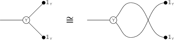
Figure 4 String diagram illustrating Claim 3.18. The claim is that the two ways of identifying the two sides of the diagram (using the symmetry of
![]() compared with the symmetry of the usual tensor product
compared with the symmetry of the usual tensor product $\otimes $
) give the same isomorphism.
$\otimes $
) give the same isomorphism.
Corollary 3.20. The ring of endomorphisms
is commutative.
Proof. This is given by a minor variant of the classical Eckmann–Hilton argument. Indeed, we note that there are two compatible multiplications on
![]() : composition and the
: composition and the
![]() product. We do not yet know that the latter is associative, but the Eckmann–Hilton argument works regardless; all we actually need is the triviality of the braiding shown in Claim 3.18.
product. We do not yet know that the latter is associative, but the Eckmann–Hilton argument works regardless; all we actually need is the triviality of the braiding shown in Claim 3.18.

3.4 Restriction to degeneracy-free representations
In this subsection, we will study the behaviour of the product
![]() on degeneracy-free representations. These will turn out to be the representations generated under colimits from the unit
on degeneracy-free representations. These will turn out to be the representations generated under colimits from the unit
![]() . Our main result (Theorem 3.26) will be that
. Our main result (Theorem 3.26) will be that
![]() behaves as a tensor product over the center of
behaves as a tensor product over the center of $\operatorname {\mathrm {Mod}}(G)$
when restricted to degeneracy-free representations, and in particular it can be extended uniquely to a symmetric monoidal structure on these representations.
$\operatorname {\mathrm {Mod}}(G)$
when restricted to degeneracy-free representations, and in particular it can be extended uniquely to a symmetric monoidal structure on these representations.
The basic definition we will use is:
Definition 3.22. We say that a module $M\in \operatorname {\mathrm {Mod}}(G)$
is degenerate if
$M\in \operatorname {\mathrm {Mod}}(G)$
is degenerate if
 $$\begin{align*}\Phi^-(M)=0. \end{align*}$$
Definition 3.23. We say that a module $N\in \operatorname {\mathrm {Mod}}(G)$
is degeneracy-free if
$N\in \operatorname {\mathrm {Mod}}(G)$
is degeneracy-free if
 $$\begin{align*}\operatorname{\mathrm{Ext}}^i(N,M)=0 \end{align*}$$
for all degenerate $M\in \operatorname {\mathrm {Mod}}(G)$
and
$M\in \operatorname {\mathrm {Mod}}(G)$
and $i=0,1$
. We denote by
$i=0,1$
. We denote by $\operatorname {\mathrm {Mod}}^{{\mathrm {deg-free}}}(G)\subseteq \operatorname {\mathrm {Mod}}(G)$
the full subcategory of degeneracy-free representations.
$\operatorname {\mathrm {Mod}}^{{\mathrm {deg-free}}}(G)\subseteq \operatorname {\mathrm {Mod}}(G)$
the full subcategory of degeneracy-free representations.
Remark 3.24. Definition 3.23 deserves a more conceptual explanation. There are two equivalent descriptions of $\operatorname {\mathrm {Mod}}^{{\mathrm {deg-free}}}(G)$
that will follow from the results later in this subsection:
$\operatorname {\mathrm {Mod}}^{{\mathrm {deg-free}}}(G)$
that will follow from the results later in this subsection:
-
1. The category
$\operatorname {\mathrm {Mod}}^{{\mathrm {deg-free}}}(G)$
is the smallest full subcategory of
$\operatorname {\mathrm {Mod}}(G)$
which contains
and is closed under colimits. This will be Claim 3.33. -
2. The second description is as follows. Consider the quotient
${\mathcal {C}}$
of the category
$\operatorname {\mathrm {Mod}}(G)$
by the degenerate representations. Then the quotient functor
$\operatorname {\mathrm {Mod}}(G) \rightarrow {\mathcal {C}}$
has a left adjoint, and this left adjoint defines an equivalence between
${\mathcal {C}}$
and
$\operatorname {\mathrm {Mod}}^{{\mathrm {deg-free}}}(G)$
. This will follow from Claim 3.30 and Theorem 3.26.


Warning 3.25. Note that, while most generic irreducible representations are degeneracy-free, this is not always the case. Specifically, let ${\mathrm {St}}$
be the Steinberg representation with trivial central character. While
${\mathrm {St}}$
be the Steinberg representation with trivial central character. While ${\mathrm {St}}$
is generic, it is not degeneracy-free. Instead, let us denote by
${\mathrm {St}}$
is generic, it is not degeneracy-free. Instead, let us denote by
![]() the unique nontrivial extension of the trivial representation
the unique nontrivial extension of the trivial representation ${\mathrm {St}}$
by
${\mathrm {St}}$
by
![]() . Then
. Then
![]() is degeneracy-free.
is degeneracy-free.
For each Bernstein component c of $\operatorname {\mathrm {Mod}}(G)$
, let
$\operatorname {\mathrm {Mod}}(G)$
, let $Z^c$
be the corresponding Bernstein center. Let
$Z^c$
be the corresponding Bernstein center. Let
 $$\begin{align*}{\mathcal{Z}}=\bigoplus_c Z^c \end{align*}$$
be the direct sum of all $Z^c$
-s. This is a nonunital ring, but it is quasi-unital (this follows formally because
$Z^c$
-s. This is a nonunital ring, but it is quasi-unital (this follows formally because ${\mathcal {Z}}$
is a direct sum of unital rings). This means that it satisfies that the multiplication map
${\mathcal {Z}}$
is a direct sum of unital rings). This means that it satisfies that the multiplication map
 $$\begin{align*}{\mathcal{Z}}\otimes_{\mathcal{Z}}{\mathcal{Z}} \rightarrow {\mathcal{Z}} \end{align*}$$
is an isomorphism. Here, $\otimes _{\mathcal {Z}}$
denotes the relative tensor product over
$\otimes _{\mathcal {Z}}$
denotes the relative tensor product over ${\mathcal {Z}}$
: That is, for a pair of (nonunital)
${\mathcal {Z}}$
: That is, for a pair of (nonunital) ${\mathcal {Z}}$
-modules M and N, the space
${\mathcal {Z}}$
-modules M and N, the space $M\otimes _{\mathcal {Z}} N$
is the quotient of
$M\otimes _{\mathcal {Z}} N$
is the quotient of $M\otimes N$
by the expressions of the form
$M\otimes N$
by the expressions of the form
 $$\begin{align*}zm\otimes n-m\otimes zn,\qquad\qquad m\in M,\, n\in N,\, z\in{\mathcal{Z}}. \end{align*}$$
Denote the symmetric monoidal category of smooth (nonunital) ${\mathcal {Z}}$
-modules by
${\mathcal {Z}}$
-modules by $\operatorname {\mathrm {Mod}}({\mathcal {Z}})$
, equipped with the relative tensor product over
$\operatorname {\mathrm {Mod}}({\mathcal {Z}})$
, equipped with the relative tensor product over ${\mathcal {Z}}$
. By definition, a
${\mathcal {Z}}$
. By definition, a ${\mathcal {Z}}$
-module M is smooth if it satisfies that the action map
${\mathcal {Z}}$
-module M is smooth if it satisfies that the action map
 $$\begin{align*}{\mathcal{Z}}\otimes_{\mathcal{Z}} M \rightarrow M \end{align*}$$
is an isomorphism. Essentially, this condition means that each $m\in M$
is supported on finitely many components of
$m\in M$
is supported on finitely many components of ${\mathcal {Z}}$
. Intuitively, quasi-unital rings share many properties with unital rings, and their smooth modules take the role of unital modules. See also Section 3 of [Reference Dor5] for more details about quasi-unital rings and their smooth modules.
${\mathcal {Z}}$
. Intuitively, quasi-unital rings share many properties with unital rings, and their smooth modules take the role of unital modules. See also Section 3 of [Reference Dor5] for more details about quasi-unital rings and their smooth modules.
Note that the symmetric monoidal category $\operatorname {\mathrm {Mod}}({\mathcal {Z}})$
acts on
$\operatorname {\mathrm {Mod}}({\mathcal {Z}})$
acts on $\operatorname {\mathrm {Mod}}(G)$
. This is a fancy way of saying that the center
$\operatorname {\mathrm {Mod}}(G)$
. This is a fancy way of saying that the center $Z^{c}$
of each component c automatically acts on the objects of the component
$Z^{c}$
of each component c automatically acts on the objects of the component $\operatorname {\mathrm {Mod}}^{c}(G)$
. Our main theorem for this subsection is:
$\operatorname {\mathrm {Mod}}^{c}(G)$
. Our main theorem for this subsection is:
Theorem 3.26. The functor
is fully faithful, with essential image $\operatorname {\mathrm {Mod}}^{{\mathrm {deg-free}}}(G)$
. Moreover, this functor is weak symmetric monoidal.
$\operatorname {\mathrm {Mod}}^{{\mathrm {deg-free}}}(G)$
. Moreover, this functor is weak symmetric monoidal.
Corollary 3.27. Consider the restriction
of the weak symmetric monoidal structure of $\operatorname {\mathrm {Mod}}(G)$
to
$\operatorname {\mathrm {Mod}}(G)$
to $\operatorname {\mathrm {Mod}}^{\mathrm {deg-free}}(G)$
. Then it can be extended from a weak symmetric monoidal structure on
$\operatorname {\mathrm {Mod}}^{\mathrm {deg-free}}(G)$
. Then it can be extended from a weak symmetric monoidal structure on $\operatorname {\mathrm {Mod}}^{{\mathrm {deg-free}}}(G)$
into a symmetric monoidal structure on
$\operatorname {\mathrm {Mod}}^{{\mathrm {deg-free}}}(G)$
into a symmetric monoidal structure on $\operatorname {\mathrm {Mod}}^{{\mathrm {deg-free}}}(G)$
in an essentially unique way (that is, in a way that is unique up to a unique isomorphism).
$\operatorname {\mathrm {Mod}}^{{\mathrm {deg-free}}}(G)$
in an essentially unique way (that is, in a way that is unique up to a unique isomorphism).
Remark 3.28. Recall from Remark 3.24 that we can think of $\operatorname {\mathrm {Mod}}^{\mathrm {deg-free}}(G)$
both as a subcategory of
$\operatorname {\mathrm {Mod}}^{\mathrm {deg-free}}(G)$
both as a subcategory of $\operatorname {\mathrm {Mod}}(G)$
and as a quotient (in fact, a colocalization) of it. Theorem 3.26 says that as a subcategory, the category
$\operatorname {\mathrm {Mod}}(G)$
and as a quotient (in fact, a colocalization) of it. Theorem 3.26 says that as a subcategory, the category $\operatorname {\mathrm {Mod}}^{\mathrm {deg-free}}(G)$
is closed under
$\operatorname {\mathrm {Mod}}^{\mathrm {deg-free}}(G)$
is closed under
. However, the reader should note that the multiplication
does not descend to $\operatorname {\mathrm {Mod}}^{\mathrm {deg-free}}(G)$
as a quotient. Specifically, the trivial representation
$\operatorname {\mathrm {Mod}}^{\mathrm {deg-free}}(G)$
as a quotient. Specifically, the trivial representation
is killed by this quotient (as it is degenerate), but one can show that

is an extension of
by a Steinberg representation (so that
is the quotient). However,
is nondegenerate as $\Phi ^-$
is an exact functor (see Proposition 3.2(a) of [Reference Bernstein and Zelevinsky3]) and
$\Phi ^-$
is an exact functor (see Proposition 3.2(a) of [Reference Bernstein and Zelevinsky3]) and ${\mathrm {St}}$
is nondegenerate. Thus, there are products of degenerate representations that are not degenerate.
${\mathrm {St}}$
is nondegenerate. Thus, there are products of degenerate representations that are not degenerate.
3.4.1 Proof of Theorem 3.26
The rest of this subsection is structured as follows. After introducing some notation, we will state Claims 3.30, 3.32 and 3.33. This will let us prove Theorem 3.26. Finally, we will prove the three claims.
Observe that the functor
 $$\begin{align*}\Phi^-{\,:\,}\operatorname{\mathrm{Mod}}(G) \rightarrow {\mathrm{Vect}} \end{align*}$$
factors through the forgetful functor $\operatorname {\mathrm {Mod}}({\mathcal {Z}}) \rightarrow {\mathrm {Vect}}$
:
$\operatorname {\mathrm {Mod}}({\mathcal {Z}}) \rightarrow {\mathrm {Vect}}$
:

In other words, because ${\mathcal {Z}}$
acts on
${\mathcal {Z}}$
acts on $\operatorname {\mathrm {Mod}}(G)$
, the spaces
$\operatorname {\mathrm {Mod}}(G)$
, the spaces $\Phi ^-(V)$
for
$\Phi ^-(V)$
for $V\in \operatorname {\mathrm {Mod}}(G)$
are canonically
$V\in \operatorname {\mathrm {Mod}}(G)$
are canonically ${\mathcal {Z}}$
-modules. We denote the corresponding
${\mathcal {Z}}$
-modules. We denote the corresponding ${\mathcal {Z}}$
-module by
${\mathcal {Z}}$
-module by $\Phi _{\mathrm {enh}}^-(V)$
and say that
$\Phi _{\mathrm {enh}}^-(V)$
and say that $\Phi _{\mathrm {enh}}^-$
is an enhancement of
$\Phi _{\mathrm {enh}}^-$
is an enhancement of $\Phi ^-$
.
$\Phi ^-$
.
Remark 3.29. The functor $\Phi ^-$
respects all colimits because it has a right adjoint (by Proposition 3.2 of [Reference Bernstein and Zelevinsky3]). In particular,
$\Phi ^-$
respects all colimits because it has a right adjoint (by Proposition 3.2 of [Reference Bernstein and Zelevinsky3]). In particular, $\Phi _{\mathrm {enh}}^-{\,:\,}\operatorname {\mathrm {Mod}}(G) \rightarrow \operatorname {\mathrm {Mod}}({\mathcal {Z}})$
also respects all colimits.
$\Phi _{\mathrm {enh}}^-{\,:\,}\operatorname {\mathrm {Mod}}(G) \rightarrow \operatorname {\mathrm {Mod}}({\mathcal {Z}})$
also respects all colimits.
For $M,N\in \operatorname {\mathrm {Mod}}(G)$
, let
$M,N\in \operatorname {\mathrm {Mod}}(G)$
, let
 $$\begin{align*}{\mathcal{H}\mathrm{om}}(M,N)\subseteq\operatorname{\mathrm{Hom}}(M,N) \end{align*}$$
be the subset consisting of morphisms supported on finitely many Bernstein components. This is the enriched inner $\operatorname {\mathrm {Hom}}$
of
$\operatorname {\mathrm {Hom}}$
of $\operatorname {\mathrm {Mod}}(G)$
over
$\operatorname {\mathrm {Mod}}(G)$
over $\operatorname {\mathrm {Mod}}({\mathcal {Z}})$
, and we therefore think of it as an object of
$\operatorname {\mathrm {Mod}}({\mathcal {Z}})$
, and we therefore think of it as an object of $\operatorname {\mathrm {Mod}}({\mathcal {Z}})$
. Note that
$\operatorname {\mathrm {Mod}}({\mathcal {Z}})$
. Note that ${\mathcal {H}\mathrm {om}}(M,N)$
is also given by the formula
${\mathcal {H}\mathrm {om}}(M,N)$
is also given by the formula
 $$\begin{align*}{\mathcal{H}\mathrm{om}}(M,N)={\mathcal{Z}}\otimes_{Z(\operatorname{\mathrm{Mod}}(G))}\operatorname{\mathrm{Hom}}(M,N) \end{align*}$$
where $Z(\operatorname {\mathrm {Mod}}(G))$
is the usual Bernstein center of
$Z(\operatorname {\mathrm {Mod}}(G))$
is the usual Bernstein center of $\operatorname {\mathrm {Mod}}(G)$
.
$\operatorname {\mathrm {Mod}}(G)$
.
We will prove Theorem 3.26 by the combination of the following three claims:
Claim 3.30. The functor
is left adjoint to
 $$\begin{align*}\Phi_{\mathrm{enh}}^-{\,:\,}\operatorname{\mathrm{Mod}}(G) \rightarrow \operatorname{\mathrm{Mod}}({\mathcal{Z}}). \end{align*}$$
Remark 3.31. This adjunction depends on our choice of Haar measure on U.
Claim 3.32. The natural map of rings induced by the action of ${\mathcal {Z}}$
on
${\mathcal {Z}}$
on $\operatorname {\mathrm {Mod}}(G)$
:
$\operatorname {\mathrm {Mod}}(G)$
:
is an isomorphism.
Claim 3.33. The smallest full subcategory of $\operatorname {\mathrm {Mod}}(G)$
containing
$\operatorname {\mathrm {Mod}}(G)$
containing
![]() and closed under all colimits is
and closed under all colimits is $\operatorname {\mathrm {Mod}}^{{\mathrm {deg-free}}}(G)$
.
$\operatorname {\mathrm {Mod}}^{{\mathrm {deg-free}}}(G)$
.
Remark 3.34. Note that Claim 3.30 is equivalent to the statement that there is a natural isomorphism of functors:
Using Claims 3.30, 3.32 and 3.33, we can now prove our main theorem.
Proof of Theorem 3.26
Claim 3.30 implies that the functor
is left adjoint to $\Phi _{\mathrm {enh}}^-$
. Remark 3.29 and Claim 3.32 show that the unit
$\Phi _{\mathrm {enh}}^-$
. Remark 3.29 and Claim 3.32 show that the unit
is an isomorphism, because
by Claim 3.32 and Remark 3.34.
The characterization of the essential image follows from Claim 3.33.
The isomorphism of Construction 3.16 now induces the requisite natural isomorphism between $\otimes _{\mathcal {Z}}$
and
$\otimes _{\mathcal {Z}}$
and
![]() . This is because
. This is because $\otimes _{\mathcal {Z}}$
is the unique colimit preserving
$\otimes _{\mathcal {Z}}$
is the unique colimit preserving ${\mathcal {Z}}$
-linear weakly symmetric monoidal structure on
${\mathcal {Z}}$
-linear weakly symmetric monoidal structure on $\operatorname {\mathrm {Mod}}({\mathcal {Z}})$
with unit
$\operatorname {\mathrm {Mod}}({\mathcal {Z}})$
with unit ${\mathcal {Z}}$
, while
${\mathcal {Z}}$
, while
![]() is
is ${\mathcal {Z}}$
-linear by Lemma 2.17 and weakly symmetric monoidal by Corollary 3.21.
${\mathcal {Z}}$
-linear by Lemma 2.17 and weakly symmetric monoidal by Corollary 3.21.
Let us now prove the three claims.
Proof of Claim 3.30
We want to construct a natural isomorphism:
for $M\in \operatorname {\mathrm {Mod}}(G)$
. Using the Haar measure on U (as in Remark 3.15), we can construct the map (essentially taking a matrix coefficient)
$M\in \operatorname {\mathrm {Mod}}(G)$
. Using the Haar measure on U (as in Remark 3.15), we can construct the map (essentially taking a matrix coefficient)

This integral takes values in $S(G)$
because of the following argument. We may suppose that f and
$S(G)$
because of the following argument. We may suppose that f and $f'$
are indicator functions for a compact neighborhood
$f'$
are indicator functions for a compact neighborhood $K_n$
of
$K_n$
of $1$
. In order for the integral to be nonzero, g must be of the form
$1$
. In order for the integral to be nonzero, g must be of the form $k^{-1}wu^{-1}k'$
for
$k^{-1}wu^{-1}k'$
for $k,k'\in K_n$
. However, the integral is also equal to
$k,k'\in K_n$
. However, the integral is also equal to $0$
for large values of u using a standard argument of multiplying k and
$0$
for large values of u using a standard argument of multiplying k and $k'$
by diagonal matrices close to
$k'$
by diagonal matrices close to $1$
.
$1$
.
This map factors through the relative tensor product over the center of $\operatorname {\mathrm {Mod}}(G)$
, and thus induces a map of modules over the center:
$\operatorname {\mathrm {Mod}}(G)$
, and thus induces a map of modules over the center:
This map factors through
.
Therefore, we have a map
which we want to prove is an isomorphism. Note that it is sufficient to prove this for M supported on a single component c, in which case
![]() .
.
The map of equation (3.5) is very nearly an isomorphism for reasons of abstract nonsense. That is, a naïve expectation would be that this immediately follows by Frobenius reciprocity. The problem, essentially, is about the smoothness of the module M. That is, the object
![]() is given by the
is given by the $\theta $
-invariants of the roughening of M, defined to be the nonsmooth
$\theta $
-invariants of the roughening of M, defined to be the nonsmooth $S(G)$
-module
$S(G)$
-module $\operatorname {\mathrm {Hom}}(S(G),M)$
.
$\operatorname {\mathrm {Hom}}(S(G),M)$
.
However, by the description of the left adjoint to $\Phi ^-$
as a functor
$\Phi ^-$
as a functor $\operatorname {\mathrm {Mod}}(P) \rightarrow {\mathrm {Vect}}$
, given in Subsection 3.2 of [Reference Bernstein and Zelevinsky3], we get
$\operatorname {\mathrm {Mod}}(P) \rightarrow {\mathrm {Vect}}$
, given in Subsection 3.2 of [Reference Bernstein and Zelevinsky3], we get

where $S(F^\times )$
is identified with the space of
$S(F^\times )$
is identified with the space of $\theta $
-coinvariants of
$\theta $
-coinvariants of $S(P)$
with respect to the right action of U on
$S(P)$
with respect to the right action of U on $S(P)$
.
$S(P)$
.
Therefore, the claim follows from Lemma 3.35 below.
Lemma 3.35. Let $M\in \operatorname {\mathrm {Mod}}^c(G)$
belong to a single component c of
$M\in \operatorname {\mathrm {Mod}}^c(G)$
belong to a single component c of $\operatorname {\mathrm {Mod}}(G)$
. Then the natural map
$\operatorname {\mathrm {Mod}}(G)$
. Then the natural map
 $$ \begin{align} M \rightarrow S(P)\otimes_{S(P)}\operatorname{\mathrm{Hom}}_G(S(G),M) \end{align} $$
becomes an isomorphism after applying $\Phi ^-$
.
$\Phi ^-$
.
Proof. We must prove that the cokernel of the map in equation (3.6) is U-invariant.
To do this, it is sufficient to consider a representation M given by compact induction:
 $$\begin{align*}M=\operatorname{\mathrm{cInd}}_K^G(\sigma) \end{align*}$$
from a representation $(\sigma ,V)$
of
$(\sigma ,V)$
of $K/K_0$
, where
$K/K_0$
, where $K={\mathrm {GL}}_2({\mathcal {O}}_F)$
and
$K={\mathrm {GL}}_2({\mathcal {O}}_F)$
and $K_0\subseteq K$
is some fixed normal compact open subset.
$K_0\subseteq K$
is some fixed normal compact open subset.
In this case, $S(P)\otimes _{S(P)}\operatorname {\mathrm {Hom}}(S(G),M)$
is the space of functions
$S(P)\otimes _{S(P)}\operatorname {\mathrm {Hom}}(S(G),M)$
is the space of functions $f{\,:\,} G \rightarrow V$
which are
$f{\,:\,} G \rightarrow V$
which are $\sigma $
-equivariant on the left, P-smooth on the right and such that the convolution
$\sigma $
-equivariant on the left, P-smooth on the right and such that the convolution
![]() from the right is compactly supported for all compact open
from the right is compactly supported for all compact open $K'\subseteq K$
.
$K'\subseteq K$
.
Pick a sufficiently large compact open subset $U^{(0)}\subseteq U$
. Replace f with its average
$U^{(0)}\subseteq U$
. Replace f with its average $\tilde {f}$
given by
$\tilde {f}$
given by
 $$\begin{align*}\tilde{f}(g)=\int_{U^{(0)}}f(gu)\theta(u^{-1}){\,\mathrm{d}{u}}. \end{align*}$$
Then $\tilde {f}(g)$
is supported on the g-s of the form
$\tilde {f}(g)$
is supported on the g-s of the form
 $$\begin{align*}k\begin{pmatrix}a & \\ & d\end{pmatrix}\begin{pmatrix}1 & b \\ & 1\end{pmatrix},\qquad k\in K \end{align*}$$
with bounded ${\left |{b}\right |}$
and
${\left |{b}\right |}$
and ${\left |{d/a}\right |}$
. However, this is sufficient to guarantee that
${\left |{d/a}\right |}$
. However, this is sufficient to guarantee that $\tilde {f}$
is G-smooth on the right, and thus compactly supported. This means that
$\tilde {f}$
is G-smooth on the right, and thus compactly supported. This means that $\tilde {f}$
is already in M.
$\tilde {f}$
is already in M.
Proof of Claim 3.32
It is sufficient to prove that the map
from the center of $\operatorname {\mathrm {Mod}}(G)$
to the endomorphisms of
$\operatorname {\mathrm {Mod}}(G)$
to the endomorphisms of
is an isomorphism.
Observe that the natural isomorphism
of Construction 3.16 induces a map from
to the endomorphisms of the identity functor of $\operatorname {\mathrm {Mod}}(G)$
, which gives a section to the above map.
$\operatorname {\mathrm {Mod}}(G)$
, which gives a section to the above map.
Therefore, it remains to prove that an element of the center of $\operatorname {\mathrm {Mod}}(G)$
which maps to
$\operatorname {\mathrm {Mod}}(G)$
which maps to $0$
in
$0$
in
![]() is
is $0$
. Indeed,
$0$
. Indeed,
![]() maps surjectively onto generic irreducible representations, and elements of the center of
maps surjectively onto generic irreducible representations, and elements of the center of $\operatorname {\mathrm {Mod}}(G)$
can be tested for equality on each irreducible generic representation separately.
$\operatorname {\mathrm {Mod}}(G)$
can be tested for equality on each irreducible generic representation separately.
Proof of Claim 3.33
It is clear that $\operatorname {\mathrm {Mod}}^{{\mathrm {deg-free}}}(G)$
is closed under colimits and contains
$\operatorname {\mathrm {Mod}}^{{\mathrm {deg-free}}}(G)$
is closed under colimits and contains
. Let $M\in \operatorname {\mathrm {Mod}}^{{\mathrm {deg-free}}}(G)$
. We want to show that it is generated under colimits from
$M\in \operatorname {\mathrm {Mod}}^{{\mathrm {deg-free}}}(G)$
. We want to show that it is generated under colimits from
. Note that Claim 3.30 and Remark 3.29 imply that
is projective. Thus, the cokernel of
is degenerate. Since $\operatorname {\mathrm {Hom}}(M,N)=0$
for all degenerate N, we conclude that p is surjective.
$\operatorname {\mathrm {Hom}}(M,N)=0$
for all degenerate N, we conclude that p is surjective.
Let the kernel of p be K. Since K also satisfies that $\operatorname {\mathrm {Hom}}(K,N)=0$
for all degenerate N, we see that M can be written as the colimit
$\operatorname {\mathrm {Hom}}(K,N)=0$
for all degenerate N, we see that M can be written as the colimit
3.5 Restriction to spherical representations
Our ultimate goal in this section is to turn
![]() into a symmetric monoidal structure on the whole of
into a symmetric monoidal structure on the whole of $\operatorname {\mathrm {Mod}}(G)$
in a canonical way. Corollary 3.27 already tells us that this is true on a large subcategory of
$\operatorname {\mathrm {Mod}}(G)$
in a canonical way. Corollary 3.27 already tells us that this is true on a large subcategory of $\operatorname {\mathrm {Mod}}(G)$
. However, it turns out that this is not enough to guarantee associativity in general. In fact, it is not difficult to construct a different weak symmetric monoidal structure
$\operatorname {\mathrm {Mod}}(G)$
. However, it turns out that this is not enough to guarantee associativity in general. In fact, it is not difficult to construct a different weak symmetric monoidal structure
![]() which has the same unit as
which has the same unit as
![]() and identifies with it on
and identifies with it on $\operatorname {\mathrm {Mod}}^{\mathrm {deg-free}}(G)$
, but which is not associative.
$\operatorname {\mathrm {Mod}}^{\mathrm {deg-free}}(G)$
, but which is not associative.
Thus, in order to prove associativity for
![]() in general, we must find a larger category on which we know that
in general, we must find a larger category on which we know that
![]() is associative. Once we have found such a sufficiently large category, the associativity of
is associative. Once we have found such a sufficiently large category, the associativity of
![]() will become a property that can be checked, instead of additional data (see Subsection 3.6).
will become a property that can be checked, instead of additional data (see Subsection 3.6).
In Subsection 3.4, we studied the restriction of
![]() to the subcategory generated by
to the subcategory generated by
![]() . It makes sense that this was not sufficient as
. It makes sense that this was not sufficient as
![]() does not generate all of
does not generate all of $\operatorname {\mathrm {Mod}}(G)$
. Thus, our goal for this subsection is to study the restriction of
$\operatorname {\mathrm {Mod}}(G)$
. Thus, our goal for this subsection is to study the restriction of
![]() to the subcategory generated by another projective object E, such that together with
to the subcategory generated by another projective object E, such that together with
![]() they generate all of
they generate all of $\operatorname {\mathrm {Mod}}(G)$
.
$\operatorname {\mathrm {Mod}}(G)$
.
Our choice of E will eventually (Remark 3.56) turn out to be a coalgebra
such that the comultiplication map $\mu $
is an isomorphism. This will force E to be coassociative, which will enable us to uniquely define the associativity data of
$\mu $
is an isomorphism. This will force E to be coassociative, which will enable us to uniquely define the associativity data of
in Subsection 3.6.
Definition 3.36. Denote ${\mathcal {O}}={\mathcal {O}}_F$
, and let K be the maximal compact subgroup
${\mathcal {O}}={\mathcal {O}}_F$
, and let K be the maximal compact subgroup ${\mathrm {GL}}_2({\mathcal {O}})$
. We let K act on the space
${\mathrm {GL}}_2({\mathcal {O}})$
. We let K act on the space $S({\mathcal {O}}^\times )$
by the determinant action. Let
$S({\mathcal {O}}^\times )$
by the determinant action. Let
 $$\begin{align*}E=\operatorname{\mathrm{cInd}}_K^G(S({\mathcal{O}}^\times)) \end{align*}$$
be the G-module given by induction with compact support of $S({\mathcal {O}}^\times )$
.
$S({\mathcal {O}}^\times )$
.
We denote the smallest full subcategory of $\operatorname {\mathrm {Mod}}(G)$
which contains E and is closed under colimits by
$\operatorname {\mathrm {Mod}}(G)$
which contains E and is closed under colimits by $\operatorname {\mathrm {Mod}}^{\mathrm {sph}}(G)$
. We refer to objects of
$\operatorname {\mathrm {Mod}}^{\mathrm {sph}}(G)$
. We refer to objects of $\operatorname {\mathrm {Mod}}^{\mathrm {sph}}(G)$
as spherical representations.
$\operatorname {\mathrm {Mod}}^{\mathrm {sph}}(G)$
as spherical representations.
Remark 3.37. Note that the term ‘spherical representations’ is not standard terminology.
Remark 3.38. We can identify
Remark 3.39. We have the natural adjunction
 $$\begin{align*}\operatorname{\mathrm{Hom}}(E,M)\cong \operatorname{\mathrm{Hom}}(S(G),M)^{\operatorname{\mathrm{SL}}_2({\mathcal{O}})}. \end{align*}$$
As a result, in order to define a map from E to a G-module M, one needs to give a $\operatorname {\mathrm {SL}}_2({\mathcal {O}})$
-invariant element of the roughening of M, defined to be the (nonsmooth)
$\operatorname {\mathrm {SL}}_2({\mathcal {O}})$
-invariant element of the roughening of M, defined to be the (nonsmooth) $S(G)$
-module
$S(G)$
-module $\operatorname {\mathrm {Hom}}(S(G),M)$
. When M is given by functions on some space, we will sometimes abuse notation and think of such elements as
$\operatorname {\mathrm {Hom}}(S(G),M)$
. When M is given by functions on some space, we will sometimes abuse notation and think of such elements as $\operatorname {\mathrm {SL}}_2({\mathcal {O}})$
-invariant distributions (although we will also fully write them out to retain clarity).
$\operatorname {\mathrm {SL}}_2({\mathcal {O}})$
-invariant distributions (although we will also fully write them out to retain clarity).
Informally, since our elements of the roughening are $\operatorname {\mathrm {SL}}_2({\mathcal {O}})$
-invariant, they are only really rough in the direction of the determinant
$\operatorname {\mathrm {SL}}_2({\mathcal {O}})$
-invariant, they are only really rough in the direction of the determinant $\det (g)$
. Hence, we will frequently use the distribution
$\det (g)$
. Hence, we will frequently use the distribution $\delta _y(y')$
defined on
$\delta _y(y')$
defined on $F^\times $
via the its standard measure under which
$F^\times $
via the its standard measure under which ${\mathcal {O}}^\times $
has volume
${\mathcal {O}}^\times $
has volume $1$
.
$1$
.
In particular, in addition to the measure on G required to give $S(G)$
its ring structure, our constructions in this subsection will only depend on the measure on
$S(G)$
its ring structure, our constructions in this subsection will only depend on the measure on $F^\times $
.
$F^\times $
.
Remark 3.40. Conceptually, the reason that E turns out to be a cocommutative coalgebra is related to the multiplicity one property of spherical vectors.
Remark 3.41. Observe that E is supported only on Bernstein components of $\operatorname {\mathrm {Mod}}(G)$
which contain a one-dimensional representation.
$\operatorname {\mathrm {Mod}}(G)$
which contain a one-dimensional representation.
Let
 $$\begin{align*}{\mathcal{Z}}_{\mathrm{sph}}=\bigoplus_{c \text{ spherical}} Z^c \end{align*}$$
be the direct sum of the Bernstein centers of all components that contain a one-dimensional representation. We think of ${\mathcal {Z}}_{\mathrm {sph}}$
as a smooth
${\mathcal {Z}}_{\mathrm {sph}}$
as a smooth ${\mathcal {Z}}$
-module, with
${\mathcal {Z}}$
-module, with ${\mathcal {Z}}$
as in Subsection 3.4. Note that
${\mathcal {Z}}$
as in Subsection 3.4. Note that ${\mathcal {Z}}_{\mathrm {sph}}$
is also quasi-unital. Denote the symmetric monoidal category of smooth
${\mathcal {Z}}_{\mathrm {sph}}$
is also quasi-unital. Denote the symmetric monoidal category of smooth ${\mathcal {Z}}_{\mathrm {sph}}$
-modules by
${\mathcal {Z}}_{\mathrm {sph}}$
-modules by $\operatorname {\mathrm {Mod}}({\mathcal {Z}}_{\mathrm {sph}})$
, and observe that
$\operatorname {\mathrm {Mod}}({\mathcal {Z}}_{\mathrm {sph}})$
, and observe that $\operatorname {\mathrm {Mod}}({\mathcal {Z}})$
acts on
$\operatorname {\mathrm {Mod}}({\mathcal {Z}})$
acts on $\operatorname {\mathrm {Mod}}({\mathcal {Z}}_{\mathrm {sph}})$
.
$\operatorname {\mathrm {Mod}}({\mathcal {Z}}_{\mathrm {sph}})$
.
Our main theorem for this subsection is
Theorem 3.42. The functor
 $$\begin{align*}-\otimes_{{\mathcal{Z}}_{\mathrm{sph}}}E{\,:\,}\operatorname{\mathrm{Mod}}({\mathcal{Z}}_{\mathrm{sph}}) \rightarrow \operatorname{\mathrm{Mod}}(G) \end{align*}$$
is fully faithful, with essential image $\operatorname {\mathrm {Mod}}^{{\mathrm {sph}}}(G)$
. Moreover, this functor sends the unit
$\operatorname {\mathrm {Mod}}^{{\mathrm {sph}}}(G)$
. Moreover, this functor sends the unit ${\mathcal {Z}}_{\mathrm {sph}}\in \operatorname {\mathrm {Mod}}({\mathcal {Z}}_{\mathrm {sph}})$
and relative tensor product
${\mathcal {Z}}_{\mathrm {sph}}\in \operatorname {\mathrm {Mod}}({\mathcal {Z}}_{\mathrm {sph}})$
and relative tensor product $\otimes _{{\mathcal {Z}}_{\mathrm {sph}}}$
to E and
$\otimes _{{\mathcal {Z}}_{\mathrm {sph}}}$
to E and
![]() , respectively.
, respectively.
Remark 3.43. We do not actually claim that the functor of Theorem 3.42 is weak symmetric monoidal as it does not respect the unit.
The proof of this theorem follows the same outline as the proof of Theorem 3.26, only easier. It is clear that E is projective, that its restriction to each component is compact and that
 $$\begin{align*}{\mathcal{Z}}_{\mathrm{sph}} \rightarrow {\mathcal{H}\mathrm{om}}(E,E) \end{align*}$$
is an isomorphism. Thus, Theorem 3.42 would immediately follow if we could prove the existence of an isomorphism
This isomorphism will be the content of Claim 3.49.
We begin by constructing a counit map
![]() , as well as constructing a comultiplication map
, as well as constructing a comultiplication map
![]() . The comultiplication
. The comultiplication $\mu $
will then be the desired isomorphism
$\mu $
will then be the desired isomorphism
![]() . Recall that
. Recall that $e{\,:\,} F \rightarrow {\mathbb {C}}^\times $
is our chosen additive character.
$e{\,:\,} F \rightarrow {\mathbb {C}}^\times $
is our chosen additive character.
Construction 3.44. Let $\nu (e)$
be the largest integer such that
$\nu (e)$
be the largest integer such that $e(\pi ^{-\nu (e)}{\mathcal {O}})=1$
, with
$e(\pi ^{-\nu (e)}{\mathcal {O}})=1$
, with $\pi \in {\mathcal {O}}$
a uniformizer. We let the map
$\pi \in {\mathcal {O}}$
a uniformizer. We let the map
be given as follows.
Let f be the distribution on G given by the delta distribution
 $$\begin{align*}f(g)=e(b)\delta_1(\det(k)) \end{align*}$$
if g has the form
 $$\begin{align*}\begin{pmatrix}1 & b \\ & 1\end{pmatrix}\begin{pmatrix}1 & \\ & -\pi^{\nu(e)}\end{pmatrix}k \end{align*}$$
with $k\in {\mathrm {GL}}_2({\mathcal {O}})$
, and we set
$k\in {\mathrm {GL}}_2({\mathcal {O}})$
, and we set $f(g)=0$
otherwise. It is clear that f is compactly supported modulo U, left-
$f(g)=0$
otherwise. It is clear that f is compactly supported modulo U, left- $\operatorname {\mathrm {SL}}_2({\mathcal {O}})$
-invariant, and right-
$\operatorname {\mathrm {SL}}_2({\mathcal {O}})$
-invariant, and right- $\theta $
-equivariant.
$\theta $
-equivariant.
Therefore, f defines an $\operatorname {\mathrm {SL}}_2({\mathcal {O}})$
-invariant element of the roughening
$\operatorname {\mathrm {SL}}_2({\mathcal {O}})$
-invariant element of the roughening $\operatorname {\mathrm {Hom}}(S(G),\operatorname {\mathrm {cInd}}_U^G(\theta ))$
given explicitly by
$\operatorname {\mathrm {Hom}}(S(G),\operatorname {\mathrm {cInd}}_U^G(\theta ))$
given explicitly by
 $$\begin{align*}\phi(g)\mapsto\int_U\int_{\operatorname{\mathrm{SL}}_2({\mathcal{O}})}e(-b)\phi\left(k^{-1}\begin{pmatrix}1 & \\ & -\pi^{-\nu(e)}\end{pmatrix}\begin{pmatrix}1 & b \\ & 1\end{pmatrix}g\right){\,\mathrm{d}^\times\!{k}}{\,\mathrm{d}{b}}. \end{align*}$$
By the universal property in Remark 3.39, we conclude that the distribution f defines a map $\varepsilon {\,:\,} E \rightarrow \operatorname {\mathrm {cInd}}_U^G(\theta )$
. Note that the resulting map
$\varepsilon {\,:\,} E \rightarrow \operatorname {\mathrm {cInd}}_U^G(\theta )$
. Note that the resulting map
![]() is independent of the choice of measure on U.
is independent of the choice of measure on U.
Construction 3.45. Let ${Y}^{\operatorname {\mathrm {SL}}_2({\mathcal {O}})\times \operatorname {\mathrm {SL}}_2({\mathcal {O}})}$
be the space of vectors in Y which are invariant under the left and right actions of
${Y}^{\operatorname {\mathrm {SL}}_2({\mathcal {O}})\times \operatorname {\mathrm {SL}}_2({\mathcal {O}})}$
be the space of vectors in Y which are invariant under the left and right actions of $\operatorname {\mathrm {SL}}_2({\mathcal {O}})$
. We let
$\operatorname {\mathrm {SL}}_2({\mathcal {O}})$
. We let $\mu $
be the map
$\mu $
be the map
given as in Remark 3.39 by the $S_3\ltimes \operatorname {\mathrm {SL}}_2({\mathcal {O}})^3$
-invariant distribution (more precisely,
$S_3\ltimes \operatorname {\mathrm {SL}}_2({\mathcal {O}})^3$
-invariant distribution (more precisely, $\operatorname {\mathrm {SL}}_2({\mathcal {O}})$
-invariant element of the roughening of
$\operatorname {\mathrm {SL}}_2({\mathcal {O}})$
-invariant element of the roughening of $Y^{\operatorname {\mathrm {SL}}_2({\mathcal {O}})\times \operatorname {\mathrm {SL}}_2({\mathcal {O}})}$
)
$Y^{\operatorname {\mathrm {SL}}_2({\mathcal {O}})\times \operatorname {\mathrm {SL}}_2({\mathcal {O}})}$
)
for $(g,y)\in \operatorname {\mathrm {M}}_2(F)\times F^\times $
. This can be more explicitly described as the
$(g,y)\in \operatorname {\mathrm {M}}_2(F)\times F^\times $
. This can be more explicitly described as the $\operatorname {\mathrm {SL}}_2({\mathcal {O}})$
-invariant element of
$\operatorname {\mathrm {SL}}_2({\mathcal {O}})$
-invariant element of $\operatorname {\mathrm {Hom}}(S(G),Y^{\operatorname {\mathrm {SL}}_2(O)\times \operatorname {\mathrm {SL}}_2({\mathcal {O}})})$
given by
$\operatorname {\mathrm {Hom}}(S(G),Y^{\operatorname {\mathrm {SL}}_2(O)\times \operatorname {\mathrm {SL}}_2({\mathcal {O}})})$
given by

where $\pi $
denotes the middle action on Y.
$\pi $
denotes the middle action on Y.
Remark 3.46. Let us try to informally motivate Constructions 3.44 and 3.45. Because the comultiplication determines the counit, we can focus on trying to understand the map $\mu $
. It turns out that
$\mu $
. It turns out that $\mu $
is related to the standard ‘distinguished test function’ on
$\mu $
is related to the standard ‘distinguished test function’ on $\operatorname {\mathrm {M}}_2(F)$
appearing in the theory of Godement–Jacquet L-functions.
$\operatorname {\mathrm {M}}_2(F)$
appearing in the theory of Godement–Jacquet L-functions.
Let us give more details. In the theory of Godement–Jacquet L-functions, it is known that if one wants to define the L-function of an unramified representation, then it is sufficient to consider the specific test function
and to integrate it against a matrix coefficient made up of unramified vectors. Our claim is that these data manifest in our theory as the comultiplication on E. Indeed, observe that in the case of $\nu (e)=0$
, the comultiplication
$\nu (e)=0$
, the comultiplication $\mu $
corresponds to the distribution
$\mu $
corresponds to the distribution
For more on this, see Remark 3.56. The same idea will also let us define the convolution product on the space of spherical automorphic functions in Section 4.
Remark 3.47. When $\nu (e)\neq 0$
, the choice of the matrix
$\nu (e)\neq 0$
, the choice of the matrix
 $$\begin{align*}\begin{pmatrix}1 & \\ & -\pi^{\nu(e)}\end{pmatrix} \end{align*}$$
in the definition of the counit
![]() in Construction 3.44 seems fairly arbitrary. Indeed, any matrix
in Construction 3.44 seems fairly arbitrary. Indeed, any matrix $h\in {\mathrm {GL}}_2(F)$
satisfying
$h\in {\mathrm {GL}}_2(F)$
satisfying
 $$\begin{align*}hKh^{-1}\cap U=\ker(\theta) \end{align*}$$
would have worked after appropriate modifications to
![]() in Construction 3.45 (i.e., using the distribution
in Construction 3.45 (i.e., using the distribution
![]() ). These data, together with the choice of the additive character
). These data, together with the choice of the additive character $e{\,:\,} F \rightarrow {\mathbb {C}}^\times $
defining
$e{\,:\,} F \rightarrow {\mathbb {C}}^\times $
defining $\theta $
, are related to something called an unramified spin structure. The precise details of this relationship will be explored in Appendix A.
$\theta $
, are related to something called an unramified spin structure. The precise details of this relationship will be explored in Appendix A.
Remark 3.48. The comultiplication
is symmetric. That is, the diagram

commutes.
We now show that
![]() and
and
![]() are consistent with being the comultiplication and counit of a coalgebra. As discussed above, the following claim immediately implies Theorem 3.42.
are consistent with being the comultiplication and counit of a coalgebra. As discussed above, the following claim immediately implies Theorem 3.42.
Claim 3.49. The diagram

commutes. Moreover, the map
![]() is an isomorphism.
is an isomorphism.
Remark 3.50. It does not yet make sense to ask about the coassociativity of $\mu $
since we have not assigned associativity data to
$\mu $
since we have not assigned associativity data to
![]() . Once we do so in Subsection 3.6 below, we will be able to upgrade Claim 3.49 and show that E is a cocommutative counital coalgebra. See also Remark 3.56.
. Once we do so in Subsection 3.6 below, we will be able to upgrade Claim 3.49 and show that E is a cocommutative counital coalgebra. See also Remark 3.56.
Proof of Claim 3.49
In order to prove that diagram (3.7) commutes, it suffices to evaluate it for the roughenings of the respective objects. Specifically, one may evaluate the two compositions on the object of the roughening of E given informally by the uniform distribution of volume $1$
on
$1$
on $\operatorname {\mathrm {SL}}_2({\mathcal {O}})$
as this generates all of E. Under
$\operatorname {\mathrm {SL}}_2({\mathcal {O}})$
as this generates all of E. Under $\mu $
, this distribution maps into
$\mu $
, this distribution maps into
We wish to apply the map $\varepsilon $
, followed by the isomorphism of Construction 3.16, and then compare the result with the delta distribution on
$\varepsilon $
, followed by the isomorphism of Construction 3.16, and then compare the result with the delta distribution on $\operatorname {\mathrm {SL}}_2({\mathcal {O}})$
, from which we started. We do so via the formula in equation (3.3); plugging
$\operatorname {\mathrm {SL}}_2({\mathcal {O}})$
, from which we started. We do so via the formula in equation (3.3); plugging $\Psi $
and
$\Psi $
and $\varepsilon $
in, we must show that
$\varepsilon $
in, we must show that
 $$\begin{align*}\int_{\operatorname{\mathrm{SL}}_2({\mathcal{O}})}\left(w\begin{pmatrix}1 & \\ & -\pi^{\nu(e)}\end{pmatrix}^{-T}k^{-T}\cdot\Psi\right)\left(g^{-1},-\det(g)\right){\,\mathrm{d}^\times\!{k}} \end{align*}$$
is the uniform distribution of volume $1$
on
$1$
on $\operatorname {\mathrm {SL}}_2({\mathcal {O}})$
.
$\operatorname {\mathrm {SL}}_2({\mathcal {O}})$
.
However, because $\Psi $
is
$\Psi $
is $\operatorname {\mathrm {SL}}_2({\mathcal {O}})$
-invariant, the above simplifies to
$\operatorname {\mathrm {SL}}_2({\mathcal {O}})$
-invariant, the above simplifies to

and we deduce that this is indeed the desired distribution from
 $$\begin{align*}\operatorname{\mathrm{M}}_2({\mathcal{O}})\cap\operatorname{\mathrm{SL}}_2(F)=\operatorname{\mathrm{SL}}_2({\mathcal{O}}). \end{align*}$$
It remains to show that $\mu $
is an isomorphism. Let us start by noting that applying the functor
$\mu $
is an isomorphism. Let us start by noting that applying the functor $\Phi ^-_{\mathrm {enh}}$
to
$\Phi ^-_{\mathrm {enh}}$
to $\mu $
, we obtain a retract of
$\mu $
, we obtain a retract of ${\mathcal {Z}}_{\mathrm {sph}}$
-modules
${\mathcal {Z}}_{\mathrm {sph}}$
-modules

Since $I_{RL}(E)\otimes _G E\cong {\mathcal {Z}}_{\mathrm {sph}}$
has no nontrivial retracts when restricted to any component, we deduce that
$I_{RL}(E)\otimes _G E\cong {\mathcal {Z}}_{\mathrm {sph}}$
has no nontrivial retracts when restricted to any component, we deduce that $\Phi ^-(\mu )$
is an isomorphism.
$\Phi ^-(\mu )$
is an isomorphism.
Having shown that $\Phi ^-$
takes the map
$\Phi ^-$
takes the map $\mu $
into an isomorphism, we see that the cokernel of
$\mu $
into an isomorphism, we see that the cokernel of $\mu $
is degenerate. However, this cokernel must be split (diagram (3.7) splits it), and it is easy to see that Y has no degenerate subrepresentations. Indeed, because Y consists of smooth and compactly supported functions on
$\mu $
is degenerate. However, this cokernel must be split (diagram (3.7) splits it), and it is easy to see that Y has no degenerate subrepresentations. Indeed, because Y consists of smooth and compactly supported functions on $\operatorname {\mathrm {M}}_2(F)\times F^\times $
, it is clear that it has no vector invariant under the action of U.
$\operatorname {\mathrm {M}}_2(F)\times F^\times $
, it is clear that it has no vector invariant under the action of U.
We can also combine Theorem 3.26 and Theorem 3.42 as follows. Consider the category
 $$\begin{align*}\operatorname{\mathrm{Mod}}({\mathcal{Z}})\times\operatorname{\mathrm{Mod}}({\mathcal{Z}}_{\mathrm{sph}}) \end{align*}$$
whose objects are pairs $(M,N)$
of smooth
$(M,N)$
of smooth ${\mathcal {Z}}$
-modules M and smooth
${\mathcal {Z}}$
-modules M and smooth ${\mathcal {Z}}_{\mathrm {sph}}$
-modules N. Recall that we are thinking of
${\mathcal {Z}}_{\mathrm {sph}}$
-modules N. Recall that we are thinking of ${\mathcal {Z}}_{\mathrm {sph}}$
as a
${\mathcal {Z}}_{\mathrm {sph}}$
as a ${\mathcal {Z}}$
-module. This category admits a unique colimit preserving symmetric monoidal structure which respects the action of
${\mathcal {Z}}$
-module. This category admits a unique colimit preserving symmetric monoidal structure which respects the action of ${\mathcal {Z}}$
, whose unit is
${\mathcal {Z}}$
, whose unit is $({\mathcal {Z}},0)$
and such that
$({\mathcal {Z}},0)$
and such that $(0,{\mathcal {Z}}_{\mathrm {sph}})$
is idempotent. This symmetric monoidal structure is explicitly defined by
$(0,{\mathcal {Z}}_{\mathrm {sph}})$
is idempotent. This symmetric monoidal structure is explicitly defined by
 $$ \begin{align*} (M_0,N_0)\otimes(M_1,N_1) \rightarrow (M_0\otimes_{\mathcal{Z}} M_1,\quad & M_0\otimes_{\mathcal{Z}} N_1 \\ \oplus & N_0\otimes_{\mathcal{Z}} M_1 \\ \oplus & N_0\otimes_{{\mathcal{Z}}}N_1). \end{align*} $$
We now conclude that
Corollary 3.51. The faithful functor
 $$\begin{align*}\operatorname{\mathrm{Mod}}({\mathcal{Z}})\times\operatorname{\mathrm{Mod}}({\mathcal{Z}}_{\mathrm{sph}}) \rightarrow \operatorname{\mathrm{Mod}}(G) \end{align*}$$
given by
is weak symmetric monoidal.
3.6 Associativity of
In this subsection, we will finally prove that
![]() uniquely extends to a symmetric monoidal structure.
uniquely extends to a symmetric monoidal structure.
Our main theorem is thus:
Theorem 3.52. There is a unique extension of
![]() from a weak symmetric monoidal structure to a symmetric monoidal structure on
from a weak symmetric monoidal structure to a symmetric monoidal structure on $\operatorname {\mathrm {Mod}}(G)$
.
$\operatorname {\mathrm {Mod}}(G)$
.
Remark 3.53. In the previous subsection, we made some choice of isomorphism
![]() . Because this was a noncanonical choice (see Remark 3.47), we had some ugly expressions. However, while in this subsection we will need to use the existence of such an isomorphism
. Because this was a noncanonical choice (see Remark 3.47), we had some ugly expressions. However, while in this subsection we will need to use the existence of such an isomorphism
![]() , our extension of
, our extension of
![]() to a symmetric monoidal structure will be unique, and in particular it will not depend on the choice of isomorphism. In other words, the effects of this choice are confined to Subsection 3.5, with the exception of Remarks 3.56 and 3.57, which are not a part of the proof of Theorem 3.52.
to a symmetric monoidal structure will be unique, and in particular it will not depend on the choice of isomorphism. In other words, the effects of this choice are confined to Subsection 3.5, with the exception of Remarks 3.56 and 3.57, which are not a part of the proof of Theorem 3.52.
Before proving Theorem 3.52, let us present some nice consequences of our constructions.
Remark 3.54. The symmetric monoidal structure
![]() on
on $\operatorname {\mathrm {Mod}}(G)$
is a part of a slightly more sophisticated higher-categorical structure called a commutative Frobenius algebra in
$\operatorname {\mathrm {Mod}}(G)$
is a part of a slightly more sophisticated higher-categorical structure called a commutative Frobenius algebra in ${\mathbb {C}}$
-linear presentable categories.
${\mathbb {C}}$
-linear presentable categories.
Specifically, the functor $\Phi ^-{\,:\,}\operatorname {\mathrm {Mod}}(G) \rightarrow {\mathrm {Vect}}$
is a trace map on
$\Phi ^-{\,:\,}\operatorname {\mathrm {Mod}}(G) \rightarrow {\mathrm {Vect}}$
is a trace map on $\operatorname {\mathrm {Mod}}(G)$
. This is because its composition with the multiplication
$\operatorname {\mathrm {Mod}}(G)$
. This is because its composition with the multiplication
is the pairing $M\boxtimes N\mapsto I_{RL}(M)\otimes _G N$
(see Remark 3.17), which is a self-duality on
$M\boxtimes N\mapsto I_{RL}(M)\otimes _G N$
(see Remark 3.17), which is a self-duality on $\operatorname {\mathrm {Mod}}(G)$
in the following higher-categorical sense.
$\operatorname {\mathrm {Mod}}(G)$
in the following higher-categorical sense.
The $2$
-category of
$2$
-category of ${\mathbb {C}}$
-linear presentable categories with colimit preserving functors is a symmetric monoidal
${\mathbb {C}}$
-linear presentable categories with colimit preserving functors is a symmetric monoidal $2$
-category, whose product is given by the Lurie tensor product. In this context,
$2$
-category, whose product is given by the Lurie tensor product. In this context,
![]() is a bilinear pairing from the category
is a bilinear pairing from the category $\operatorname {\mathrm {Mod}}(G)$
to the unit
$\operatorname {\mathrm {Mod}}(G)$
to the unit ${\mathrm {Vect}}$
of the symmetric monoidal structure, and it is easy to see that this is in fact a perfect pairing.
${\mathrm {Vect}}$
of the symmetric monoidal structure, and it is easy to see that this is in fact a perfect pairing.
Example 3.55. We can now give a much cleaner reformulation and proof of Theorem 2.2. For any object $V\in \operatorname {\mathrm {Mod}}(G)$
, we have a canonical morphism
$V\in \operatorname {\mathrm {Mod}}(G)$
, we have a canonical morphism
Theorem 2.2 can be simply stated as saying that, for a generic irreducible representation V, the above is an isomorphism. Note that this implies that after a choice of Whittaker model (i.e., an isomorphism
), we have
.
In fact, something even stronger can be said: After fixing a nonzero vector $v^{\mathrm {gen}}$
in the one-dimensional space
$v^{\mathrm {gen}}$
in the one-dimensional space
a generic irreducible representation V canonically becomes a unital commutative algebra with respect to
.
Moreover, this strengthening of Theorem 2.2 now has an exceedingly short proof. Indeed, it immediately follows from the following general principle. Let ${\mathcal {C}}$
be a symmetric monoidal abelian category with a right exact tensor product. Then all surjections
${\mathcal {C}}$
be a symmetric monoidal abelian category with a right exact tensor product. Then all surjections
![]() from the unit induce isomorphisms
from the unit induce isomorphisms $X\xrightarrow {\sim } X\otimes X$
, and moreover turn X into a commutative unital algebra.
$X\xrightarrow {\sim } X\otimes X$
, and moreover turn X into a commutative unital algebra.
Remark 3.56. Using the idempotent theorem of [Reference Gurevich and Hadani9], it is an easy observation that Theorem 3.52 and Claim 3.49 imply that E is necessarily coassociative. That is, E is a counital cocommutative coalgebra with respect to
![]() .
.
This has the following implication. Fix a choice of comultiplication on E as in Remark 3.47 (recall that these data can be derived from a global spin structure, a fact explored in detail in Appendix A). Let V be any unital and commutative algebra with respect to
![]() . Then the space
. Then the space $V_{/\operatorname {\mathrm {SL}}_2({\mathcal {O}})}={\mathcal {H}\mathrm {om}}(E,V)$
of coinvariants is automatically a quasi-unital commutative algebra over
$V_{/\operatorname {\mathrm {SL}}_2({\mathcal {O}})}={\mathcal {H}\mathrm {om}}(E,V)$
of coinvariants is automatically a quasi-unital commutative algebra over ${\mathcal {Z}}_{\mathrm {sph}}$
, with respect to the usual tensor product
${\mathcal {Z}}_{\mathrm {sph}}$
, with respect to the usual tensor product $\otimes $
(note that invariants and coinvariants with respect to
$\otimes $
(note that invariants and coinvariants with respect to $\operatorname {\mathrm {SL}}_2({\mathcal {O}})$
are the same since the group is compact). In the global setting, this will let us define a multiplicative structure on a certain space of spherical automorphic functions. See Appendix A for details.
$\operatorname {\mathrm {SL}}_2({\mathcal {O}})$
are the same since the group is compact). In the global setting, this will let us define a multiplicative structure on a certain space of spherical automorphic functions. See Appendix A for details.
Informally, the product of $V_{/\operatorname {\mathrm {SL}}_2({\mathcal {O}})}$
comes from the product of V using the ‘distinguished test function’ appearing in the definition of the comultiplication of E in Construction 3.45. That is, to multiply two vectors of
$V_{/\operatorname {\mathrm {SL}}_2({\mathcal {O}})}$
comes from the product of V using the ‘distinguished test function’ appearing in the definition of the comultiplication of E in Construction 3.45. That is, to multiply two vectors of $V_{/\operatorname {\mathrm {SL}}_2({\mathcal {O}})}$
, one tensors them with the distinguished test function and then applies the product of V. See also Remark 3.46.
$V_{/\operatorname {\mathrm {SL}}_2({\mathcal {O}})}$
, one tensors them with the distinguished test function and then applies the product of V. See also Remark 3.46.
Remark 3.57. We can say something even stronger. As in Remark 3.47, fix a choice of comultiplication on E, and let V be any unital and commutative algebra with respect to
as above. Note that
is also a coalgebra. Thus, the space
can also be automatically upgraded into a quasi-unital commutative algebra over the center ${\mathcal {Z}}$
(with respect to the usual tensor product
${\mathcal {Z}}$
(with respect to the usual tensor product $\otimes $
). Moreover, the following diagram of algebras commutes:
$\otimes $
). Moreover, the following diagram of algebras commutes:

For V a generic irreducible representation as in Example 3.55, this is not very interesting as $\Phi ^-V$
and
$\Phi ^-V$
and $V_{/\operatorname {\mathrm {SL}}_2({\mathcal {O}})}$
are both at most one-dimensional. However, this will be a much more interesting statement for
$V_{/\operatorname {\mathrm {SL}}_2({\mathcal {O}})}$
are both at most one-dimensional. However, this will be a much more interesting statement for $V={\mathscr {I}}$
, the algebra of automorphic functions developed in Section 4. See also Appendix A.
$V={\mathscr {I}}$
, the algebra of automorphic functions developed in Section 4. See also Appendix A.
The rest of this subsection is dedicated to the proof of Theorem 3.52. We begin with the following strengthening of Corollary 3.51.
Claim 3.58. There is at most one extension of
![]() from a weak symmetric monoidal structure to a symmetric monoidal structure on
from a weak symmetric monoidal structure to a symmetric monoidal structure on $\operatorname {\mathrm {Mod}}(G)$
. Moreover, the functor
$\operatorname {\mathrm {Mod}}(G)$
. Moreover, the functor
 $$\begin{align*}\operatorname{\mathrm{Mod}}({\mathcal{Z}})\times\operatorname{\mathrm{Mod}}({\mathcal{Z}}_{\mathrm{sph}}) \rightarrow \operatorname{\mathrm{Mod}}(G) \end{align*}$$
of Corollary 3.51 is symmetric monoidal for any such extension.
Proof. Consider any extension of
![]() to a symmetric monoidal structure (that is, suppose that there is some associator for
to a symmetric monoidal structure (that is, suppose that there is some associator for
![]() satisfying the axioms of a symmetric monoidal structure).
satisfying the axioms of a symmetric monoidal structure).
We want to show that any two such extensions are equal. Because
respects colimits, it is enough to compare their associators
on objects $A,B,C$
that are either of the two generators
$A,B,C$
that are either of the two generators
. Note that if any of the objects $A,B,C$
is equal to
$A,B,C$
is equal to
, then the associator is uniquely determined by unitality.
Thus, it remains to show that the only possible choice for the associator
is the one coming from the functor
 $$\begin{align*}\operatorname{\mathrm{Mod}}({\mathcal{Z}})\times\operatorname{\mathrm{Mod}}({\mathcal{Z}}_{\mathrm{sph}}) \rightarrow \operatorname{\mathrm{Mod}}(G). \end{align*}$$
That is, it remains to show that the only possible choice for the associator
is the identification
coming from repeated applications of Claim 3.49.
Indeed, in this case the pentagonal axiom

fully determines the associator; any such associator must be given by a map $a{\,:\,} E\xrightarrow {\sim } E$
(after using Claim 3.49 to identify
$a{\,:\,} E\xrightarrow {\sim } E$
(after using Claim 3.49 to identify
), which must then satisfy
 $$\begin{align*}a^2=a^3. \end{align*}$$
Note that this is the same argument as the idempotent theorem (Theorem 3.1.2) of [Reference Gurevich and Hadani9].
Proof of Theorem 3.52
The functor
 $$\begin{align*}\iota{\,:\,}\operatorname{\mathrm{Mod}}({\mathcal{Z}})\times\operatorname{\mathrm{Mod}}({\mathcal{Z}}_{\mathrm{sph}}) \rightarrow \operatorname{\mathrm{Mod}}(G) \end{align*}$$
defines associator isomorphisms
for $A,B,C\in \operatorname {\mathrm {Mod}}({\mathcal {Z}})\times \operatorname {\mathrm {Mod}}({\mathcal {Z}}_{\mathrm {sph}})$
, by considering the images of the associators in its domain. Note that, because
$A,B,C\in \operatorname {\mathrm {Mod}}({\mathcal {Z}})\times \operatorname {\mathrm {Mod}}({\mathcal {Z}}_{\mathrm {sph}})$
, by considering the images of the associators in its domain. Note that, because $\iota $
is not fully faithful, this family of isomorphisms does not automatically descend to its essential image.
$\iota $
is not fully faithful, this family of isomorphisms does not automatically descend to its essential image.
Let ${\mathcal {C}}_0\subseteq \operatorname {\mathrm {Mod}}(G)$
be the fully faithful subcategory given by finite direct sums of
${\mathcal {C}}_0\subseteq \operatorname {\mathrm {Mod}}(G)$
be the fully faithful subcategory given by finite direct sums of
and E. Because
is a ${\mathcal {Z}}$
-linear functor that respects colimits, it is uniquely determined by its restriction to
${\mathcal {Z}}$
-linear functor that respects colimits, it is uniquely determined by its restriction to ${\mathcal {C}}_0$
. Indeed,
${\mathcal {C}}_0$
. Indeed, $\operatorname {\mathrm {Mod}}(G)$
is generated as a
$\operatorname {\mathrm {Mod}}(G)$
is generated as a ${\mathcal {Z}}$
-linear category by
${\mathcal {Z}}$
-linear category by
and E. In fact,
is given by the left Kan extension
Thus, it is sufficient to show that the associators $a_{A,B,C}$
commute with the morphisms of
$a_{A,B,C}$
commute with the morphisms of $\operatorname {\mathrm {Mod}}(G)$
on the finite direct sums of
$\operatorname {\mathrm {Mod}}(G)$
on the finite direct sums of ${\mathcal {Z}}$
and
${\mathcal {Z}}$
and ${\mathcal {Z}}_{\mathrm {sph}}$
in
${\mathcal {Z}}_{\mathrm {sph}}$
in $\operatorname {\mathrm {Mod}}({\mathcal {Z}})\times \operatorname {\mathrm {Mod}}({\mathcal {Z}}_{\mathrm {sph}})$
, and therefore induce a natural morphism on
$\operatorname {\mathrm {Mod}}({\mathcal {Z}})\times \operatorname {\mathrm {Mod}}({\mathcal {Z}}_{\mathrm {sph}})$
, and therefore induce a natural morphism on ${\mathcal {C}}_0$
. The required compatibilities with the rest of the symmetric monoidal structure (and the pentagonal axiom) will follow immediately from those of
${\mathcal {C}}_0$
. The required compatibilities with the rest of the symmetric monoidal structure (and the pentagonal axiom) will follow immediately from those of $\operatorname {\mathrm {Mod}}({\mathcal {Z}})\times \operatorname {\mathrm {Mod}}({\mathcal {Z}}_{\mathrm {sph}})$
.
$\operatorname {\mathrm {Mod}}({\mathcal {Z}})\times \operatorname {\mathrm {Mod}}({\mathcal {Z}}_{\mathrm {sph}})$
.
Because $\operatorname {\mathrm {Mod}}({\mathcal {Z}})\times \operatorname {\mathrm {Mod}}({\mathcal {Z}}_{\mathrm {sph}})$
is generated under colimits by
$\operatorname {\mathrm {Mod}}({\mathcal {Z}})\times \operatorname {\mathrm {Mod}}({\mathcal {Z}}_{\mathrm {sph}})$
is generated under colimits by
and E, it is sufficient to prove that for all
and all maps $f{\,:\,} C \rightarrow D$
, the following diagram commutes:
$f{\,:\,} C \rightarrow D$
, the following diagram commutes:

The claim follows immediately if either A or B is
![]() . Additionally, because
. Additionally, because
![]() respects the action of the center and because both
respects the action of the center and because both
![]() and
and ${\mathrm {End}}(E)$
are covered by the center, it is enough to consider the case
${\mathrm {End}}(E)$
are covered by the center, it is enough to consider the case $C\neq D$
, so either
$C\neq D$
, so either
![]() or
or
![]() .
.
Since the proof in either case is identical, it is enough to consider the case
. Letting
, we must show that the following diagram commutes:

We can rewrite this as the following diagram commuting:

which is equivalent to asking that the two maps
given by
and
be equal.
In other words, it is sufficient to prove that the map
 $$\begin{align*}\operatorname{\mathrm{Hom}}(E,E) \rightarrow \operatorname{\mathrm{Hom}}(E,E) \end{align*}$$
given by
is the identity map of $\operatorname {\mathrm {Hom}}(E,E)$
. But the center of
$\operatorname {\mathrm {Hom}}(E,E)$
. But the center of $\operatorname {\mathrm {Mod}}(G)$
covers
$\operatorname {\mathrm {Mod}}(G)$
covers $\operatorname {\mathrm {Hom}}(E,E)$
. Therefore, it is enough to test this property on the identity map of E, and verify that
$\operatorname {\mathrm {Hom}}(E,E)$
. Therefore, it is enough to test this property on the identity map of E, and verify that
However, this holds by functoriality of
.
Part II
Abstractly automorphic representations
4 Global automorphic forms
4.1 Introduction
Our goal for this section is to observe that an appropriate space of automorphic functions becomes a commutative algebra under the symmetric monoidal structure
![]() .
.
Let F be a global function field of characteristic $\neq 2$
. Fix the standard Haar measure
$\neq 2$
. Fix the standard Haar measure ${\,\mathrm {d}^\times \!{g}} $
on
${\,\mathrm {d}^\times \!{g}} $
on ${\mathbb {A}}^\times $
(respectively,
${\mathbb {A}}^\times $
(respectively, ${\mathrm {GL}}_2({\mathbb {A}})$
) such that the product of the maximal compact subgroups
${\mathrm {GL}}_2({\mathbb {A}})$
) such that the product of the maximal compact subgroups ${\mathcal {O}}_v^\times $
(respectively,
${\mathcal {O}}_v^\times $
(respectively, ${\mathrm {GL}}_2({\mathcal {O}}_v)$
) is of measure
${\mathrm {GL}}_2({\mathcal {O}}_v)$
) is of measure $1$
.
$1$
.
Consider the space
of automorphic functions – smooth and compactly supported functions on the automorphic quotient ${\mathrm {GL}}_2(F)\backslash {\mathrm {GL}}_2({\mathbb {A}})$
. Let
${\mathrm {GL}}_2(F)\backslash {\mathrm {GL}}_2({\mathbb {A}})$
. Let
be the projection along the determinant map
 $$\begin{align*}\det{\,:\,}{\mathrm{GL}}_2({\mathbb{A}}) \rightarrow {\mathbb{A}}^\times, \end{align*}$$
and let ${\mathscr {I}}$
be the kernel of p (note that
${\mathscr {I}}$
be the kernel of p (note that ${\mathscr {I}}$
is independent of the choices of Haar measures). Given any two functions
${\mathscr {I}}$
is independent of the choices of Haar measures). Given any two functions
and a test function $\Psi \in S(\operatorname {\mathrm {M}}_2({\mathbb {A}}))$
, one obtains a Godement–Jacquet zeta integral
$\Psi \in S(\operatorname {\mathrm {M}}_2({\mathbb {A}}))$
, one obtains a Godement–Jacquet zeta integral
 $$ \begin{align*} Z_{\text{GJ}}\left(\phi',\phi,\Psi,s\right)=\int_{{\mathrm{GL}}_2({\mathbb{A}})}\left(\int_{{\mathrm{GL}}_2(F)\backslash{\mathrm{GL}}_2({\mathbb{A}})}\phi'(h^{-T})\phi(hg){\,\mathrm{d}^\times\!{h}}\right)\Psi(g){\left|{\det(g)}\right|}^{s+\frac{1}{2}}{\,\mathrm{d}^\times\!{g}}. \end{align*} $$
On the other hand, a single function
with Whittaker function $W_{\phi "}$
also has an associated Jacquet–Langlands zeta integral
$W_{\phi "}$
also has an associated Jacquet–Langlands zeta integral
 $$\begin{align*}Z_{\text{JL}}\left(\phi",s\right)=\int_{{\mathbb{A}}^\times}W_{\phi"}\left(\begin{pmatrix}y & \\ & 1\end{pmatrix}\right){\left|{y}\right|}^{s-\frac{1}{2}}{\,\mathrm{d}^\times\!{y}}. \end{align*}$$
Below, we will see that the equality of Godement–Jacquet and Jacquet–Langlands L-functions more or less induces a multiplication map on
. More precisely, we will obtain a map
on the kernel ${\mathscr {I}}$
of
${\mathscr {I}}$
of
which turns Godement–Jacquet zeta integrals into Jacquet–Langlands zeta integrals. We will show that this multiplication map makes ${\mathscr {I}}$
into a commutative unital algebra with respect to the symmetric monoidal structure
${\mathscr {I}}$
into a commutative unital algebra with respect to the symmetric monoidal structure
.
To put this construction in context inside the theory of automorphic representations, one can think about the multiplication map we construct as a kind of theta lifting of pairs of automorphic forms. This is essentially a shadow of the construction of Y in Section 2 as a Weil representation.
Before delving into the structure of this section, let us detail some more of the remarkable properties of the algebra ${\mathscr {I}}$
. For starters, it turns out that the unit map
${\mathscr {I}}$
. For starters, it turns out that the unit map
is surjective. This implies that while the multiplication map uniquely determines the unit, the other direction holds as well. In fact, for any smooth ${\mathrm {GL}}_2({\mathbb {A}})$
-module V, being an
${\mathrm {GL}}_2({\mathbb {A}})$
-module V, being an ${\mathscr {I}}$
-module is a mere property, equivalent to the existence of a (necessarily unique) lift
${\mathscr {I}}$
-module is a mere property, equivalent to the existence of a (necessarily unique) lift

It turns out that
, along with all irreducible automorphic representations, are ${\mathscr {I}}$
-modules. This justifies thinking of the property of being an
${\mathscr {I}}$
-modules. This justifies thinking of the property of being an ${\mathscr {I}}$
-module as an automorphicity property. In fact, it appears that the category
${\mathscr {I}}$
-module as an automorphicity property. In fact, it appears that the category $\operatorname {\mathrm {Mod}}^{\mathrm {aut}}({\mathrm {GL}}_2({\mathbb {A}}))$
of
$\operatorname {\mathrm {Mod}}^{\mathrm {aut}}({\mathrm {GL}}_2({\mathbb {A}}))$
of ${\mathscr {I}}$
-modules is a natural context for the study of automorphic representations.
${\mathscr {I}}$
-modules is a natural context for the study of automorphic representations.
Remark 4.1. The multiplication
![]() continues the theme discussed in Remark 3.1, where the symmetric monoidal structure
continues the theme discussed in Remark 3.1, where the symmetric monoidal structure
![]() seems to mimic the behaviour of the relative tensor product over a commutative group. That is, over a commutative group H, the space of functions on a quotient
seems to mimic the behaviour of the relative tensor product over a commutative group. That is, over a commutative group H, the space of functions on a quotient $\Gamma \backslash H$
of the group carries a convolution product. Intuitively, it seems as though the multiplication on
$\Gamma \backslash H$
of the group carries a convolution product. Intuitively, it seems as though the multiplication on ${\mathscr {I}}$
takes the same role as this convolution product, despite the group
${\mathscr {I}}$
takes the same role as this convolution product, despite the group ${\mathrm {GL}}_2({\mathbb {A}})$
being noncommutative. The cost of this noncommutativity is the use of the exotic symmetric monoidal structure
${\mathrm {GL}}_2({\mathbb {A}})$
being noncommutative. The cost of this noncommutativity is the use of the exotic symmetric monoidal structure
![]() .
.
One can think of the structure of this section as one big construction of the algebra structure on ${\mathscr {I}}$
. Let us be more specific.
${\mathscr {I}}$
. Let us be more specific.
We start in Subsection 4.2, where we fix some definitions for
![]() in the global case as we have only discussed
in the global case as we have only discussed
![]() locally so far.
locally so far.
In Subsection 4.3, we will define the desired multiplication map. In fact, we will construct a single multiplication map
![]() into the contragradient
into the contragradient
![]() of
of
![]() (which canonically contains
(which canonically contains
![]() ). At this point, the multiplication will simply be a map; we will not even know if the subspace
). At this point, the multiplication will simply be a map; we will not even know if the subspace
![]() is closed under multiplication.
is closed under multiplication.
In Subsection 4.4, we will show that this multiplication is unital by explicitly constructing a unit map
![]() . In Subsection 4.5, we will show that this unit map
. In Subsection 4.5, we will show that this unit map
![]() is surjective. This will imply that the multiplication we defined is associative, as well as show that
is surjective. This will imply that the multiplication we defined is associative, as well as show that ${\mathscr {I}}$
is closed under multiplication, and establish the desired algebraic structure. Finally, in Subsection 4.6, we will discuss the property of being an
${\mathscr {I}}$
is closed under multiplication, and establish the desired algebraic structure. Finally, in Subsection 4.6, we will discuss the property of being an ${\mathscr {I}}$
-module, and construct the category of abstractly automorphic representations.
${\mathscr {I}}$
-module, and construct the category of abstractly automorphic representations.
Having established our desired constructions, in Appendix A we will fulfill a debt and show how the coalgebra E of Subsection 3.5 is related to global spin structures. This will allow us to show that the spherical functions in ${\mathscr {I}}$
are an algebra with respect to the usual tensor product
${\mathscr {I}}$
are an algebra with respect to the usual tensor product $\otimes $
, as described in Section 1.
$\otimes $
, as described in Section 1.
4.2 Global symmetric monoidal structure
We begin by turning the local symmetric monoidal structures
![]() at each place
at each place $F_v$
into a global symmetric monoidal structure
$F_v$
into a global symmetric monoidal structure
![]() on the category
on the category $\operatorname {\mathrm {Mod}}({\mathrm {GL}}_2({\mathbb {A}}))$
of smooth
$\operatorname {\mathrm {Mod}}({\mathrm {GL}}_2({\mathbb {A}}))$
of smooth ${\mathrm {GL}}_2({\mathbb {A}})$
-modules.
${\mathrm {GL}}_2({\mathbb {A}})$
-modules.
Define
 $$\begin{align*}{Y_{\mathbb{A}}}=S(\operatorname{\mathrm{M}}_2({\mathbb{A}})\times{\mathbb{A}}^\times) \end{align*}$$
via a restricted tensor product of the local spaces $S(\operatorname {\mathrm {M}}_2(F_v)\times F_v^\times )$
, with respect to the distinguished functions
$S(\operatorname {\mathrm {M}}_2(F_v)\times F_v^\times )$
, with respect to the distinguished functions
![]() . Fix a nontrivial additive character
. Fix a nontrivial additive character $e{\,:\,}{\mathbb {A}}/F \rightarrow {\mathbb {C}}^\times $
once and for all. Using e, Construction 2.13 gives the space
$e{\,:\,}{\mathbb {A}}/F \rightarrow {\mathbb {C}}^\times $
once and for all. Using e, Construction 2.13 gives the space ${Y_{\mathbb {A}}}$
a smooth
${Y_{\mathbb {A}}}$
a smooth ${\mathrm {GL}}_2({\mathbb {A}})^3$
-action. Note that, in this section, we will allow ourselves to more implicitly switch between right and left
${\mathrm {GL}}_2({\mathbb {A}})^3$
-action. Note that, in this section, we will allow ourselves to more implicitly switch between right and left ${\mathrm {GL}}_2({\mathbb {A}})$
actions. However, we will always do so via the transposition map, as in Definition 3.2.
${\mathrm {GL}}_2({\mathbb {A}})$
actions. However, we will always do so via the transposition map, as in Definition 3.2.
We define the bifunctor
by
Here, $\otimes _G$
denotes the relative tensor product over the global group
$\otimes _G$
denotes the relative tensor product over the global group $G={\mathrm {GL}}_2({\mathbb {A}})$
.
$G={\mathrm {GL}}_2({\mathbb {A}})$
.
The global unit
![]() is defined as the
is defined as the $\theta $
-coinvariants of
$\theta $
-coinvariants of $S({\mathrm {GL}}_2({\mathbb {A}}))$
with respect to the right action of
$S({\mathrm {GL}}_2({\mathbb {A}}))$
with respect to the right action of $U({\mathbb {A}})$
, where
$U({\mathbb {A}})$
, where $\theta {\,:\,} U({\mathbb {A}})/U(F) \rightarrow {\mathbb {C}}^\times $
is given by
$\theta {\,:\,} U({\mathbb {A}})/U(F) \rightarrow {\mathbb {C}}^\times $
is given by
 $$\begin{align*}\theta\left(\begin{pmatrix}1 & u \\ & 1\end{pmatrix}\right)=e(u). \end{align*}$$
Remark 4.2. As in Remark 3.15 in the local case, fixing a Haar measure on $U=U({\mathbb {A}})$
allows us to define an isomorphism
$U=U({\mathbb {A}})$
allows us to define an isomorphism
where $\operatorname {\mathrm {cInd}}_U^G(\theta )$
is the representation of G obtained from
$\operatorname {\mathrm {cInd}}_U^G(\theta )$
is the representation of G obtained from $\theta $
by induction with compact support.
$\theta $
by induction with compact support.
We now claim that the local commutativity, associativity and unitality data turn
![]() into a symmetric monoidal structure on
into a symmetric monoidal structure on $\operatorname {\mathrm {Mod}}({\mathrm {GL}}_2({\mathbb {A}}))$
. This requires some compatibility of the commutativity, associativity and unitality data of Section 3 with the distinguished vector
$\operatorname {\mathrm {Mod}}({\mathrm {GL}}_2({\mathbb {A}}))$
. This requires some compatibility of the commutativity, associativity and unitality data of Section 3 with the distinguished vector
![]() at each place.
at each place.
Claim 4.3. Let v be a place of F. Additionally, let $Y_v=S(\operatorname {\mathrm {M}}_2(F_v)\times F_v^\times )$
, let
$Y_v=S(\operatorname {\mathrm {M}}_2(F_v)\times F_v^\times )$
, let $G_v={\mathrm {GL}}_2(F_v)$
, and let
$G_v={\mathrm {GL}}_2(F_v)$
, and let
![]() be the distinguished vector. The following hold for almost all places v:
be the distinguished vector. The following hold for almost all places v:
-
1. The isomorphism
of Construction 3.16 sends distinguished vectors to distinguished vectors. -
2. The action of the permutation
$(1,3)$
interchanging the left and right actions on
$Y_v$
sends the distinguished vector
$y_v\in Y_v$
to itself. -
3. The associativity constraint
$Y_v\otimes _{G_v} Y_v\cong Y_v\otimes _{G_v} Y_v$
sends the distinguished vector
$y_v\otimes y_v$
to itself.


Proof. Recall that for every place v, the space
![]() is a cocommutative, counital, coalgebra by Remark 3.56. For places v where
is a cocommutative, counital, coalgebra by Remark 3.56. For places v where $e_v$
is unramified, denote by
$e_v$
is unramified, denote by $f_v$
the vector
$f_v$
the vector
![]() .
.
We observe that under the counit
![]() of Construction 3.44, the vector
of Construction 3.44, the vector $f_v$
maps to the distinguished vector
$f_v$
maps to the distinguished vector
![]() of
of
![]() . Moreover, observe that under the comultiplication map
. Moreover, observe that under the comultiplication map
![]() of Construction 3.45, the vector
of Construction 3.45, the vector $f_v$
maps to
$f_v$
maps to $f_v\otimes y_v\otimes f_v\in E_v\otimes _{G_v}Y_v\otimes _{G_v} E_v$
.
$f_v\otimes y_v\otimes f_v\in E_v\otimes _{G_v}Y_v\otimes _{G_v} E_v$
.
Therefore, the counitality of $E_v$
implies Item 1, the cocommutativity of
$E_v$
implies Item 1, the cocommutativity of $E_v$
implies Item 2, and the coassociativity of
$E_v$
implies Item 2, and the coassociativity of $E_v$
implies Item 3.
$E_v$
implies Item 3.
Corollary 4.4. The local commutativity, associativity and unitality data comprise well-defined global maps, turning
![]() into a symmetric monoidal structure on
into a symmetric monoidal structure on $\operatorname {\mathrm {Mod}}({\mathrm {GL}}_2({\mathbb {A}}))$
.
$\operatorname {\mathrm {Mod}}({\mathrm {GL}}_2({\mathbb {A}}))$
.
4.3 The
-algebra of automorphic forms
In this subsection, we will define the promised multiplication map
Later, in Subsection 4.5, we will show an associativity-type statement for it, as well as prove that the image of
lies inside ${\mathscr {I}}$
. This will turn
${\mathscr {I}}$
. This will turn ${\mathscr {I}}$
into an algebra.
${\mathscr {I}}$
into an algebra.
Let us begin with an informal discussion. We are trying to construct a map
which sends Godement–Jacquet zeta integrals to Jacquet–Langlands zeta integrals. This map should take as input pairs of automorphic functions, as well as a test function from ${Y_{\mathbb {A}}}$
, and yield an element of
${Y_{\mathbb {A}}}$
, and yield an element of
. We think of the codomain
as the space of smooth functions on ${\mathrm {GL}}_2(F)\backslash {\mathrm {GL}}_2({\mathbb {A}})$
, without any conditions on growth. The Godement–Jacquet zeta integral of the input data (two automorphic functions and a test function) should be the same as the Jacquet–Langlands zeta integral of the output (a smooth function on
${\mathrm {GL}}_2(F)\backslash {\mathrm {GL}}_2({\mathbb {A}})$
, without any conditions on growth. The Godement–Jacquet zeta integral of the input data (two automorphic functions and a test function) should be the same as the Jacquet–Langlands zeta integral of the output (a smooth function on ${\mathrm {GL}}_2(F)\backslash {\mathrm {GL}}_2({\mathbb {A}})$
). We will formalize this compatibility property in Remark 4.11.
${\mathrm {GL}}_2(F)\backslash {\mathrm {GL}}_2({\mathbb {A}})$
). We will formalize this compatibility property in Remark 4.11.
This compatibility with zeta integrals should in principle be enough to recover the multiplication map m, for the following reason. Recovering a sufficiently nice function
![]() from its family of Jacquet–Langlands zeta integrals is fairly standard. One simply integrates the zeta integrals over all unitary characters
from its family of Jacquet–Langlands zeta integrals is fairly standard. One simply integrates the zeta integrals over all unitary characters $\chi {\,:\,}{\mathbb {A}}^\times /F^\times \rightarrow {\mathbb {C}}^\times $
(i.e., applies the inverse Mellin transform) to isolate
$\chi {\,:\,}{\mathbb {A}}^\times /F^\times \rightarrow {\mathbb {C}}^\times $
(i.e., applies the inverse Mellin transform) to isolate $\phi "(1)$
. The rest of the values of
$\phi "(1)$
. The rest of the values of $\phi "$
can be recovered by the
$\phi "$
can be recovered by the ${\mathrm {GL}}_2({\mathbb {A}})$
-equivariance of the map we are trying to construct.
${\mathrm {GL}}_2({\mathbb {A}})$
-equivariance of the map we are trying to construct.
Let
denote the coinvariants of ${Y_{\mathbb {A}}}$
with respect to the left and right
${Y_{\mathbb {A}}}$
with respect to the left and right ${\mathrm {GL}}_2(F)$
-actions. The above discussion suggests defining a linear functional
${\mathrm {GL}}_2(F)$
-actions. The above discussion suggests defining a linear functional
that should informally correspond to taking the Godement–Jacquet zeta integral of the input and applying the inverse Mellin transform to it. If we did everything correctly, it will then be invariant under the middle action of ${\mathrm {GL}}_2(F)$
. With this extra invariance property, we will be able to equivariantly extend the map
${\mathrm {GL}}_2(F)$
. With this extra invariance property, we will be able to equivariantly extend the map
into the desired multiplication map
.
In other words, due to the universal property of the contragradient, it is enough to give a linear functional
 $$\begin{align*}\mu{\,:\,} {Y_{\mathbb{A}}} \rightarrow {\mathbb{C}} \end{align*}$$
which is invariant under all three actions of ${\mathrm {GL}}_2(F)$
. Note that this goal is inherently symmetric in the three actions.
${\mathrm {GL}}_2(F)$
. Note that this goal is inherently symmetric in the three actions.
The structure of the rest of this subsection is as follows. We will formally define the desired linear functional in §4.3.1. In §4.3.2, we will show that this functional is invariant under the full action of ${\mathrm {GL}}_2(F)^3$
. Finally, in §4.3.3, we will define the multiplication map
${\mathrm {GL}}_2(F)^3$
. Finally, in §4.3.3, we will define the multiplication map
![]() itself, and discuss its compatibility with zeta integrals.
itself, and discuss its compatibility with zeta integrals.
4.3.1 Defining the functional
We propose the following functional, which will be justified by Remark 4.11 below.
Definition 4.5. Define the linear functional
 $$ \begin{align*} \mu{\,:\,} {Y_{\mathbb{A}}} \rightarrow {\mathbb{C}} \end{align*} $$
by the formula
 $$\begin{align*}\mu(\Psi)\mapsto\sum_{(\xi,q)\in\operatorname{\mathrm{M}}_2(F)\times F^\times}\Psi(\xi,q). \end{align*}$$
Remark 4.6. The functional $\mu $
is clearly invariant with respect to the left and right actions of
$\mu $
is clearly invariant with respect to the left and right actions of ${\mathrm {GL}}_2(F)$
. Moreover,
${\mathrm {GL}}_2(F)$
. Moreover, $\mu $
is also invariant with respect to the middle action of
$\mu $
is also invariant with respect to the middle action of $P_2(F)$
. This follows using the explicit formula for the middle action of the mirabolic group on
$P_2(F)$
. This follows using the explicit formula for the middle action of the mirabolic group on ${Y_{\mathbb {A}}}$
given in equation (2.12).
${Y_{\mathbb {A}}}$
given in equation (2.12).
Remark 4.7. The functional $\mu $
is clearly symmetric under the action of the transposition of
$\mu $
is clearly symmetric under the action of the transposition of $\operatorname {\mathrm {M}}_2({\mathbb {A}})$
on
$\operatorname {\mathrm {M}}_2({\mathbb {A}})$
on ${Y_{\mathbb {A}}}$
(see Remark 3.4).
${Y_{\mathbb {A}}}$
(see Remark 3.4).
4.3.2 Invariance of the functional
Our goal for this subsubsection is to prove that $\mu $
is indeed invariant under all three of the
$\mu $
is indeed invariant under all three of the ${\mathrm {GL}}_2(F)$
-actions. This will give us a map
${\mathrm {GL}}_2(F)$
-actions. This will give us a map
into the smoothening
of the dual of
(i.e., the contragradient of
.
Remark 4.8. The reader should note that the strategy we are proposing looks like a kind of theta lifting. The image of
![]() in
in
![]() is essentially given by a theta function, up to issues related to the center of
is essentially given by a theta function, up to issues related to the center of ${\mathrm {GL}}_2$
.
${\mathrm {GL}}_2$
.
In fact, we prove something even stronger:
Proposition 4.9. The functional $\mu {\,:\,} {Y_{\mathbb {A}}} \rightarrow {\mathbb {C}}$
is invariant with respect to the
$\mu {\,:\,} {Y_{\mathbb {A}}} \rightarrow {\mathbb {C}}$
is invariant with respect to the $S_3\ltimes {\mathrm {GL}}_2(F)^3$
-action of Remark 3.5.
$S_3\ltimes {\mathrm {GL}}_2(F)^3$
-action of Remark 3.5.
Proof. This immediately follows from the invariance of the theta functional
 $$ \begin{align*} S(\operatorname{\mathrm{M}}_2({\mathbb{A}})) & \rightarrow {\mathbb{C}} \\ \Psi & \mapsto\sum_{\xi\in\operatorname{\mathrm{M}}_2(F)}\Psi(\xi) \end{align*} $$
under the action of the group of rational points of the metaplectic group used in the construction of ${Y_{\mathbb {A}}}$
.
${Y_{\mathbb {A}}}$
.
Nevertheless, let us explicitly show the invariance under the middle action of ${\mathrm {GL}}_2(F)$
. By Remark 4.6, it is sufficient to prove that
${\mathrm {GL}}_2(F)$
. By Remark 4.6, it is sufficient to prove that $\mu $
is invariant under the middle action of the matrix
$\mu $
is invariant under the middle action of the matrix $w=\begin {pmatrix} & -1 \\ 1 & \end {pmatrix}$
. Using Remark 2.24, it is enough to show that
$w=\begin {pmatrix} & -1 \\ 1 & \end {pmatrix}$
. Using Remark 2.24, it is enough to show that
 $$\begin{align*}\sum_{(\xi,q)\in\operatorname{\mathrm{M}}_2(F)\times F^\times}\Psi(\xi,q)=\sum_{(\xi,q)\in\operatorname{\mathrm{M}}_2(F)\times F^\times}{\left|{q}\right|}^2\int_{\operatorname{\mathrm{M}}_2(F)}\Psi(h,q)\cdot e\bigg(-q\cdot\left<\xi,h\right>\bigg){\,\mathrm{d}{h}}. \end{align*}$$
However,
 $$ \begin{align*} & \sum_{(\xi,q)\in\operatorname{\mathrm{M}}_2(F)\times F^\times}{\left|{q}\right|}^2\int_{\operatorname{\mathrm{M}}_2(F)}\Psi(h,q)\cdot e \bigg(-q\cdot\left<\xi,h\right>\bigg){\,\mathrm{d}{h}} \\ &\qquad=\sum_{(\xi,q)\in\operatorname{\mathrm{M}}_2(F)\times F^\times}\int_{\operatorname{\mathrm{M}}_2(F)}\Psi(h,q)\cdot e\bigg(-{\mathrm{tr}}(\xi^T h)\bigg){\,\mathrm{d}{h}}, \end{align*} $$
where we have used the identity
 $$\begin{align*}\left<\xi,h\right>={\mathrm{tr}}(w^{-1}\xi^T wh). \end{align*}$$
We are now done by the Poisson summation formula
 $$\begin{align*}\sum_{(\xi,q)\in\operatorname{\mathrm{M}}_2(F)\times F^\times}\Psi(\xi,q)=\sum_{(\xi,q)\in\operatorname{\mathrm{M}}_2(F)\times F^\times}\int_{\operatorname{\mathrm{M}}_2(F)}\Psi(h,q)\cdot e\bigg(-{\mathrm{tr}}(\xi^T h)\bigg){\,\mathrm{d}{h}}. \end{align*}$$
4.3.3 Defining the multiplication
Proposition 4.9 justifies the following construction.
Construction 4.10. We define a map
by composing the identification
with the map

Here, $g\cdot \Psi $
denotes the middle action.
$g\cdot \Psi $
denotes the middle action.
In our informal discussion at the beginning of this subsection, it was emphasized that the multiplication map m should be compatible with zeta integrals in some sense. Let us formalize this.
Remark 4.11. The multiplication
![]() sends Godement–Jacquet zeta integrals into Jacquet–Langlands zeta integrals. Specifically, we claim that
sends Godement–Jacquet zeta integrals into Jacquet–Langlands zeta integrals. Specifically, we claim that
 $$\begin{align*}Z_{\text{JL}}\left(m(\phi'\otimes\Psi\otimes f\otimes\phi),s\right)=Z_{\text{GJ}}\left(\phi',\phi,\Psi,s\right)\cdot\int_{{\mathbb{A}}^\times} f(y){\left|{y}\right|}^{s+\frac{1}{2}}{\,\mathrm{d}^\times\!{y}}, \end{align*}$$
where $\Psi \otimes f\in {Y_{\mathbb {A}}}$
,
$\Psi \otimes f\in {Y_{\mathbb {A}}}$
,
![]() , and
, and
 $$ \begin{align*} Z_{\text{JL}}\left(\phi",s\right) & =\int_{{\mathbb{A}}^\times} W_{\phi"}\left(\begin{pmatrix}y & \\ & 1\end{pmatrix}\right){\left|{y}\right|}^{s-\frac{1}{2}}{\,\mathrm{d}^\times\!{y}}, \\ Z_{\text{GJ}}\left(\phi',\phi,\Psi,s\right) & =\int_{{\mathrm{GL}}_2({\mathbb{A}})} \left(\int_{{\mathrm{GL}}_2(F)\backslash{\mathrm{GL}}_2({\mathbb{A}})}\phi'(h^{-T})\phi(hg) {\,\mathrm{d}^\times\!{h}}\right) \Psi(g){\left|{\det(g)}\right|}^{s+\frac{1}{2}}{\,\mathrm{d}^\times\!{g}} \end{align*} $$
are the Jacquet–Langlands and Godement–Jacquet zeta integrals, respectively. Here, $W_{\phi "}$
is the Whittaker function corresponding to
$W_{\phi "}$
is the Whittaker function corresponding to
![]() . This can be easily seen via a direct computation.
. This can be easily seen via a direct computation.
Recall that we have normalized the measures on ${\mathrm {GL}}_2({\mathbb {A}})$
and
${\mathrm {GL}}_2({\mathbb {A}})$
and ${\mathbb {A}}^\times $
in Subsection 4.1 so that they have measure
${\mathbb {A}}^\times $
in Subsection 4.1 so that they have measure $1$
on maximal compact subgroups. Also, note that it is standard to define the Whittaker function
$1$
on maximal compact subgroups. Also, note that it is standard to define the Whittaker function $W_{\phi "}$
using a measure on
$W_{\phi "}$
using a measure on $U({\mathbb {A}})$
which assigns a measure of
$U({\mathbb {A}})$
which assigns a measure of $1$
to
$1$
to $U({\mathbb {A}})/U(F)$
.
$U({\mathbb {A}})/U(F)$
.
4.4 Unitality of
In the previous subsection, we defined a multiplication map
![]() (Construction 4.10). We have not yet proven that
(Construction 4.10). We have not yet proven that
![]() maps to
maps to ${\mathscr {I}}$
, and not yet shown any associativity properties of m. In this subsection, we will discuss the unitality of the multiplication m.
${\mathscr {I}}$
, and not yet shown any associativity properties of m. In this subsection, we will discuss the unitality of the multiplication m.
Recall that in a category ${\mathcal {C}}$
with a symmetric monoidal structure
${\mathcal {C}}$
with a symmetric monoidal structure $\otimes $
, a commutative algebra object
$\otimes $
, a commutative algebra object $A\in {\mathcal {C}}$
is called unital if there exists a (necessarily unique) map
$A\in {\mathcal {C}}$
is called unital if there exists a (necessarily unique) map
such that
is the identity map.
Specifically, in this subsection, we will begin by constructing a map
![]() (which, in fact, factors through
(which, in fact, factors through ${\mathscr {I}}$
). Afterwards, we will show (Corollary 4.18) that the composition
${\mathscr {I}}$
). Afterwards, we will show (Corollary 4.18) that the composition
is the inclusion
![]() adjoint to the Petersson pairing
adjoint to the Petersson pairing
![]() . This is the desired unitality of m, which will later translate into e being the unit for the commutative algebra
. This is the desired unitality of m, which will later translate into e being the unit for the commutative algebra ${\mathscr {I}}$
with its multiplication induced by m.
${\mathscr {I}}$
with its multiplication induced by m.
Remark 4.12. We are going to give an explicit construction of the unit map e in this subsection, while in the previous subsection we gave an explicit construction for the multiplication map m. However, these two constructions are not independent and more or less determine each other.
Indeed, it should be noted that as with all algebras, the multiplication map m (given in Construction 4.10) and the unitality property (given in diagram (4.1)) are already sufficient to uniquely determine e. Moreover, in our case the other direction holds as well; this means the following. We will show in Subsection 4.5 that the unit map e has image
![]() . This will mean that the unit map e already uniquely determines the restriction of the multiplication map m to
. This will mean that the unit map e already uniquely determines the restriction of the multiplication map m to
![]() (see also Remark 4.23).
(see also Remark 4.23).
Let us begin. The cleanest way to describe the map
![]() is by looking at its dual,
is by looking at its dual,
![]() .
.
Construction 4.13. We think of
![]() as the space of smooth functions on the automorphic quotient
as the space of smooth functions on the automorphic quotient ${\mathrm {GL}}_2(F)\backslash {\mathrm {GL}}_2({\mathbb {A}})$
, and of
${\mathrm {GL}}_2(F)\backslash {\mathrm {GL}}_2({\mathbb {A}})$
, and of
![]() as the space of
as the space of $\theta ^{-1}$
-equivariant functions on
$\theta ^{-1}$
-equivariant functions on ${\mathrm {GL}}_2({\mathbb {A}})$
. We define the map
${\mathrm {GL}}_2({\mathbb {A}})$
. We define the map
![]() by sending an automorphic function to its corresponding Whittaker function:
by sending an automorphic function to its corresponding Whittaker function:
 $$\begin{align*}\phi(g)\mapsto W_\phi(g)=\int_{U({\mathbb{A}})/U(F)}\phi(ug)\theta(u){\,\mathrm{d}{u}}. \end{align*}$$
Here, we use a normalized measure on $U({\mathbb {A}})/U(F)$
such that the total volume is
$U({\mathbb {A}})/U(F)$
such that the total volume is $1$
.
$1$
.
We now claim that
Claim 4.14. There is a unique map
![]() such that its contragradient is the map
such that its contragradient is the map
![]() of Construction 4.13.
of Construction 4.13.
Indeed, it is clear that the contragradient is a faithful functor. Therefore, we can prove Claim 4.14 by directly constructing the desired map
![]() . This will be our unit for the multiplication on the algebra
. This will be our unit for the multiplication on the algebra ${\mathscr {I}}$
.
${\mathscr {I}}$
.
Construction 4.15. Define the map
as the composition of
 $$ \begin{align*} S({\mathrm{GL}}_2({\mathbb{A}}))_{/U_2({\mathbb{A}}),\theta} & \rightarrow S(U_2(F)\backslash{\mathrm{GL}}_2({\mathbb{A}})) \\ f(g) & \mapsto\int_{U_2({\mathbb{A}})}f(ug)\theta(u^{-1}){\,\mathrm{d}{u}} \end{align*} $$
with the projection
. In other words, using the equivalence of Remark 4.2, a function
is mapped to the Poincaré series

It is a standard fact that this Poincaré series is an element of $S({\mathrm {GL}}_2(F)\backslash {\mathrm {GL}}_2({\mathbb {A}}))$
.
$S({\mathrm {GL}}_2(F)\backslash {\mathrm {GL}}_2({\mathbb {A}}))$
.
The map
![]() of Construction 4.15 will be a unit with respect to the multiplication
of Construction 4.15 will be a unit with respect to the multiplication
![]() of Construction 4.10. To show this, we will need the following proposition about the Petersson pairing.
of Construction 4.10. To show this, we will need the following proposition about the Petersson pairing.
Recall that the Petersson pairing is the map
given by
 $$\begin{align*}f(g)\otimes f'(g')\mapsto\int_{{\mathrm{GL}}_2({\mathbb{A}})}f(g)f'(g^{-T}){\,\mathrm{d}^\times\!{g}} , \end{align*}$$
where we have implicitly used
instead of the more formally correct
. This can also be described by the functional

where the notation
denotes the coinvariants of the vector space $S({\mathrm {GL}}_2({\mathbb {A}}))$
under the two actions of
$S({\mathrm {GL}}_2({\mathbb {A}}))$
under the two actions of ${\mathrm {GL}}_2(F)$
.
${\mathrm {GL}}_2(F)$
.
Proposition 4.16. The composition
is the Petersson pairing $\rho $
, where
$\rho $
, where $\mu $
is the map of Definition 4.5.
$\mu $
is the map of Definition 4.5.
Remark 4.17. Proposition 4.16 is independent of which of the three copies of
![]() we insert
we insert
![]() into. This follows by the
into. This follows by the $S_3$
-invariance shown in Proposition 4.9.
$S_3$
-invariance shown in Proposition 4.9.
Finally, the desired unitality property of
![]() follows because
follows because $\mu $
is given by m together with the natural evaluation pairing.
$\mu $
is given by m together with the natural evaluation pairing.
Corollary 4.18. The composition
is the inclusion
.
Proof of Proposition 4.16
We want to show that the two maps
coincide. This is a straightforward verification. We will show that the diagram

commutes by separately evaluating the clockwise and counter-clockwise compositions.
We begin with the counterclockwise composition. Using equation (3.3), it is given by
 $$ \begin{align*} f(h)\otimes\Psi(g,y)\mapsto\sum_{\xi\in{\mathrm{GL}}_2(F)}\int_{{\mathrm{GL}}_2({\mathbb{A}})}(wh^{-T}\cdot\Psi)(\xi^{-1},-\det(\xi))\cdot f(h){\,\mathrm{d}^\times\!{h}}. \end{align*} $$
We should compare this with the clockwise composition
 $$ \begin{align*} f(h)\otimes\Psi(g,y) &\mapsto \sum_{(\xi,q)\in\operatorname{\mathrm{M}}_2(F)\times F^\times}\int_{U_2(F)\backslash{\mathrm{GL}}_2({\mathbb{A}})}\int_{U_2({\mathbb{A}})}(h^{-T}\cdot\Psi)(\xi,q)\cdot f(uh)\cdot\theta(u^{-1}){\,\mathrm{d}{u}}{\,\mathrm{d}^\times\!{h}} \\ &=\sum_{(\xi,q)\in\operatorname{\mathrm{M}}_2(F)\times F^\times}\int_{U_2(F)\backslash{\mathrm{GL}}_2({\mathbb{A}})}\int_{U_2({\mathbb{A}})}(wh^{-T}\cdot\Psi)(\xi,-q)\cdot f(uh)\cdot\theta(u^{-1}){\,\mathrm{d}{u}}{\,\mathrm{d}^\times\!{h}} \\ &=\sum_{(\xi,q)\in\operatorname{\mathrm{M}}_2(F)\times F^\times}\int_{{\mathrm{GL}}_2({\mathbb{A}})}(wh^{-T}\cdot\Psi)(\xi,-q)\cdot f(h)\cdot \int_{{\mathbb{A}}/F}e(x(q\det{\xi}-1)){\,\mathrm{d}{x}} {\,\mathrm{d}^\times\!{h}}. \end{align*} $$
Thus, the two maps coincide.
4.5 Associativity of the multiplication
We are now armed with a unital multiplication map
![]() . Our goal in this subsection will be to prove that it is associative in some sense and to prove that
. Our goal in this subsection will be to prove that it is associative in some sense and to prove that ${\mathscr {I}}$
is an algebra.
${\mathscr {I}}$
is an algebra.
Everything will immediately follow from the following proposition.
Proposition 4.19. The image of the unit map
![]() of Construction 4.15 is
of Construction 4.15 is ${\mathscr {I}}$
.
${\mathscr {I}}$
.
Remark 4.20. In a very vague sense, Proposition 4.19 can be thought of as a multiplicity one property; because a generic irreducible V has $\dim \Phi ^-V=1$
, it follows that the space of maps between
$\dim \Phi ^-V=1$
, it follows that the space of maps between ${\mathscr {I}}$
and V is at most one dimensional as well. Following the proof of Proposition 4.19 below, one can also see that it relies on similar ideas to the usual proof of multiplicity one.
${\mathscr {I}}$
and V is at most one dimensional as well. Following the proof of Proposition 4.19 below, one can also see that it relies on similar ideas to the usual proof of multiplicity one.
Before proving Proposition 4.19, let us state some of its corollaries.
Corollary 4.21. The image
![]() lies inside
lies inside
![]() .
.
Proof. Consider the commutative diagram

The left vertical map is surjective, while the right vertical map is injective. This means that the diagram can be completed as above.
Corollary 4.22. The multiplication
![]() makes
makes ${\mathscr {I}}$
into a unital commutative algebra with respect to
${\mathscr {I}}$
into a unital commutative algebra with respect to
![]() .
.
Proof. Follows immediately from the surjectivity of
and the axioms of symmetric monoidal categories. By Corollaries 4.18 and 4.21, it is sufficient to show that the multiplication
is associative. Indeed, we have two maps

and we want to show that they are the same. By Proposition 4.19, we can test this by precomposing with the unit map
at one of the coordinates. However, the two maps

are the same by the unitality result of Corollary 4.18.
Remark 4.23. In fact, the surjectivity of the unit map implies that m is the unique multiplicative structure on ${\mathscr {I}}$
with respect to this unit.
${\mathscr {I}}$
with respect to this unit.
Remark 4.24. Observe that ${\mathscr {I}}$
becomes not just an algebra, but it also carries a pairing
${\mathscr {I}}$
becomes not just an algebra, but it also carries a pairing
induced from the Petersson pairing
(here, $\Phi ^-{\,:\,}\operatorname {\mathrm {Mod}}(G) \rightarrow {\mathrm {Vect}}$
indicates the functor of
$\Phi ^-{\,:\,}\operatorname {\mathrm {Mod}}(G) \rightarrow {\mathrm {Vect}}$
indicates the functor of $\theta $
-coinvariants; recall that
$\theta $
-coinvariants; recall that $\Phi ^-$
defines a trace on the category
$\Phi ^-$
defines a trace on the category $\operatorname {\mathrm {Mod}}(G)$
, as in Remark 3.54). Moreover, the
$\operatorname {\mathrm {Mod}}(G)$
, as in Remark 3.54). Moreover, the $S_3$
-invariance shown in Proposition 4.9 implies that this map satisfies the axiom
$S_3$
-invariance shown in Proposition 4.9 implies that this map satisfies the axiom
 $$\begin{align*}\left<x,yz\right>=\left<xy,z\right>. \end{align*}$$
Note that ${\mathscr {I}}$
is not a Frobenius algebra because it is not self-dual: The map
${\mathscr {I}}$
is not a Frobenius algebra because it is not self-dual: The map ${\mathscr {I}} \rightarrow \widetilde {{\mathscr {I}}}$
induced from the pairing is not an isomorphism.
${\mathscr {I}} \rightarrow \widetilde {{\mathscr {I}}}$
induced from the pairing is not an isomorphism.
Corollary 4.25. The image
![]() lies inside
lies inside
![]() .
.
Proof. Identical to Corollary 4.21.
Corollary 4.26. The multiplication
![]() turns
turns
![]() into an
into an ${\mathscr {I}}$
-module with respect to
${\mathscr {I}}$
-module with respect to
![]() .
.
Proof. Identical to Corollary 4.22.
Remark 4.27. We have seen that we can think of the multiplication
![]() as defining an algebra structure on
as defining an algebra structure on ${\mathscr {I}}$
, and of the multiplication
${\mathscr {I}}$
, and of the multiplication
![]() as defining an
as defining an ${\mathscr {I}}$
-module structure on
${\mathscr {I}}$
-module structure on
![]() . Both of these multiplications are associative in an appropriate sense. This raises the question of how to think about the associativity of the multiplication map
. Both of these multiplications are associative in an appropriate sense. This raises the question of how to think about the associativity of the multiplication map
![]() .
.
We answer this as follows. Note that the map
defines a symmetric triality
by the universal property of the contragradient
and Remark 3.17. Our claim is that this triality respects the ${\mathscr {I}}$
-module structure of
${\mathscr {I}}$
-module structure of
. This follows immediately by the surjectivity of the map
.
We dedicate the rest of this subsection to the proof of Proposition 4.19.
Proof of Proposition 4.19
Since
it remains to show that the map
is surjective. To do so, let us show that the sequence
is exact.
We will show this by proving that the sequence of contragradients
is exact. That is, it is sufficient to show that if $\phi {\,:\,}{\mathrm {GL}}_2(F)\backslash {\mathrm {GL}}_2({\mathbb {A}}) \rightarrow {\mathbb {C}}$
is a smooth automorphic function whose corresponding Whittaker function
$\phi {\,:\,}{\mathrm {GL}}_2(F)\backslash {\mathrm {GL}}_2({\mathbb {A}}) \rightarrow {\mathbb {C}}$
is a smooth automorphic function whose corresponding Whittaker function
 $$\begin{align*}W_\phi(g)=\int_{U({\mathbb{A}})/U(F)}\phi(ug)\theta(u){\,\mathrm{d}{u}} \end{align*}$$
is $0$
, then
$0$
, then $\phi $
is
$\phi $
is $\operatorname {\mathrm {SL}}_2({\mathbb {A}})\cdot {\mathrm {GL}}_2(F)$
-invariant.
$\operatorname {\mathrm {SL}}_2({\mathbb {A}})\cdot {\mathrm {GL}}_2(F)$
-invariant.
Indeed, from $W_\phi =0$
we see that
$W_\phi =0$
we see that $\phi $
is left
$\phi $
is left $U({\mathbb {A}})$
-invariant. Since
$U({\mathbb {A}})$
-invariant. Since $\phi $
is also
$\phi $
is also ${\mathrm {GL}}_2(F)$
-invariant, it follows that
${\mathrm {GL}}_2(F)$
-invariant, it follows that $\phi $
is left-invariant with respect to the subgroup generated by
$\phi $
is left-invariant with respect to the subgroup generated by $U({\mathbb {A}})$
and
$U({\mathbb {A}})$
and ${\mathrm {GL}}_2(F)$
. However, it is easy to check that this subgroup contains
${\mathrm {GL}}_2(F)$
. However, it is easy to check that this subgroup contains $\operatorname {\mathrm {SL}}_2({\mathbb {A}})$
. This finishes the proof.
$\operatorname {\mathrm {SL}}_2({\mathbb {A}})$
. This finishes the proof.
4.6 Abstract automorphicity
The purpose of this subsection is to introduce the category $\operatorname {\mathrm {Mod}}^{\mathrm {aut}}({\mathrm {GL}}_2({\mathbb {A}}))$
of abstractly automorphic representations. This category will be a full subcategory of
$\operatorname {\mathrm {Mod}}^{\mathrm {aut}}({\mathrm {GL}}_2({\mathbb {A}}))$
of abstractly automorphic representations. This category will be a full subcategory of $\operatorname {\mathrm {Mod}}({\mathrm {GL}}_2({\mathbb {A}}))$
, containing all irreducible automorphic representations, and closed under taking subquotients and contragradients. The author’s belief is that this category is a natural place in which to study the theory of automorphic representations.
$\operatorname {\mathrm {Mod}}({\mathrm {GL}}_2({\mathbb {A}}))$
, containing all irreducible automorphic representations, and closed under taking subquotients and contragradients. The author’s belief is that this category is a natural place in which to study the theory of automorphic representations.
Let $\operatorname {\mathrm {Mod}}({\mathscr {I}})$
be the category of
$\operatorname {\mathrm {Mod}}({\mathscr {I}})$
be the category of ${\mathscr {I}}$
-modules in
${\mathscr {I}}$
-modules in $\operatorname {\mathrm {Mod}}({\mathrm {GL}}_2({\mathbb {A}}))$
. This makes sense as
$\operatorname {\mathrm {Mod}}({\mathrm {GL}}_2({\mathbb {A}}))$
. This makes sense as $\operatorname {\mathrm {Mod}}({\mathrm {GL}}_2({\mathbb {A}}))$
is a symmetric monoidal category, and
$\operatorname {\mathrm {Mod}}({\mathrm {GL}}_2({\mathbb {A}}))$
is a symmetric monoidal category, and ${\mathscr {I}}$
is an algebra with respect to its symmetric monoidal structure
${\mathscr {I}}$
is an algebra with respect to its symmetric monoidal structure
![]() . We begin by observing that:
. We begin by observing that:
Claim 4.28. The forgetful functor from $\operatorname {\mathrm {Mod}}({\mathscr {I}})$
to
$\operatorname {\mathrm {Mod}}({\mathscr {I}})$
to $\operatorname {\mathrm {Mod}}({\mathrm {GL}}_2({\mathbb {A}}))$
is fully faithful.
$\operatorname {\mathrm {Mod}}({\mathrm {GL}}_2({\mathbb {A}}))$
is fully faithful.
Proof. Follows immediately from Proposition 4.19.
This justifies giving a name to the essential image.
Definition 4.29. Let $V\in \operatorname {\mathrm {Mod}}({\mathrm {GL}}_2({\mathbb {A}}))$
. We will say that V is abstractly automorphic if V belongs to the essential image of
$V\in \operatorname {\mathrm {Mod}}({\mathrm {GL}}_2({\mathbb {A}}))$
. We will say that V is abstractly automorphic if V belongs to the essential image of $\operatorname {\mathrm {Mod}}({\mathscr {I}})$
in
$\operatorname {\mathrm {Mod}}({\mathscr {I}})$
in $\operatorname {\mathrm {Mod}}({\mathrm {GL}}_2({\mathbb {A}}))$
.
$\operatorname {\mathrm {Mod}}({\mathrm {GL}}_2({\mathbb {A}}))$
.
Denote by $\operatorname {\mathrm {Mod}}^{\mathrm {aut}}({\mathrm {GL}}_2({\mathbb {A}}))\subseteq \operatorname {\mathrm {Mod}}({\mathrm {GL}}_2({\mathbb {A}}))$
the full subcategory of abstractly automorphic representations.
$\operatorname {\mathrm {Mod}}^{\mathrm {aut}}({\mathrm {GL}}_2({\mathbb {A}}))\subseteq \operatorname {\mathrm {Mod}}({\mathrm {GL}}_2({\mathbb {A}}))$
the full subcategory of abstractly automorphic representations.
Remark 4.30. Equivalently, a smooth ${\mathrm {GL}}_2({\mathbb {A}})$
-module V is abstractly automorphic if and only if the canonical map
${\mathrm {GL}}_2({\mathbb {A}})$
-module V is abstractly automorphic if and only if the canonical map
![]() factors through the quotient
factors through the quotient
![]() .
.
Remark 4.31. Note that the above also means that the structure of
![]() as an
as an ${\mathscr {I}}$
-module observed in Corollary 4.26 is unique. That is, since Corollary 4.26 implies that
${\mathscr {I}}$
-module observed in Corollary 4.26 is unique. That is, since Corollary 4.26 implies that
![]() , it follows from Claim 4.28 that
, it follows from Claim 4.28 that
![]() carries a unique structure of
carries a unique structure of ${\mathscr {I}}$
-module.
${\mathscr {I}}$
-module.
Proposition 4.32. The category $\operatorname {\mathrm {Mod}}^{\mathrm {aut}}({\mathrm {GL}}_2({\mathbb {A}}))$
of abstractly automorphic representations is closed under taking subquotients in
$\operatorname {\mathrm {Mod}}^{\mathrm {aut}}({\mathrm {GL}}_2({\mathbb {A}}))$
of abstractly automorphic representations is closed under taking subquotients in $\operatorname {\mathrm {Mod}}({\mathrm {GL}}_2({\mathbb {A}}))$
.
$\operatorname {\mathrm {Mod}}({\mathrm {GL}}_2({\mathbb {A}}))$
.
Moreover, it is also closed under taking contragradients.
Proof. The proof is a straightforward application of Remark 4.30.
Let us show closure under taking contragradients. Let $V\in \operatorname {\mathrm {Mod}}^{\mathrm {aut}}({\mathrm {GL}}_2({\mathbb {A}}))$
. By Remark 4.30, we must show that the identity map
$V\in \operatorname {\mathrm {Mod}}^{\mathrm {aut}}({\mathrm {GL}}_2({\mathbb {A}}))$
. By Remark 4.30, we must show that the identity map $\widetilde {V} \rightarrow \widetilde {V}$
factors through
$\widetilde {V} \rightarrow \widetilde {V}$
factors through
. By the universal property of $\widetilde {V}$
, this is equivalent to showing that the pairing
$\widetilde {V}$
, this is equivalent to showing that the pairing
factors through
However, this holds by associativity of
and the abstract automorphicity of V.
Let us also show closure under taking subobjects. Closure under quotients is similar. Let V be abstractly automorphic, and let $V'\subseteq V$
. Then we have a map
$V'\subseteq V$
. Then we have a map
We claim that the image of
lies inside $V'$
. Indeed, we can check the image by precomposing with
$V'$
. Indeed, we can check the image by precomposing with
, but the map
factors through the canonical map
.
Remark 4.33. We have already seen in Corollary 4.26 that
![]() is abstractly automorphic. Therefore, so is
is abstractly automorphic. Therefore, so is
![]() , and in particular, all irreducible automorphic representations are also abstractly automorphic, being subquotients of it.
, and in particular, all irreducible automorphic representations are also abstractly automorphic, being subquotients of it.
Remark 4.34. Very informally, if we imagine objects of $\operatorname {\mathrm {Mod}}({\mathrm {GL}}_2({\mathbb {A}}))$
as sheaves on some algebraic space, then Proposition 4.19 says that
$\operatorname {\mathrm {Mod}}({\mathrm {GL}}_2({\mathbb {A}}))$
as sheaves on some algebraic space, then Proposition 4.19 says that ${\mathscr {I}}$
defines a closed subspace of that algebraic space.
${\mathscr {I}}$
defines a closed subspace of that algebraic space.
Let us elaborate on this analogy. Instead of the symmetric monoidal category $\operatorname {\mathrm {Mod}}({\mathrm {GL}}_2({\mathbb {A}}))$
equipped with
$\operatorname {\mathrm {Mod}}({\mathrm {GL}}_2({\mathbb {A}}))$
equipped with
![]() , consider the category
, consider the category $\operatorname {\mathrm {Mod}}(A)$
of A-modules for some commutative algebra A, equipped with the relative tensor product over A. Then the unit of
$\operatorname {\mathrm {Mod}}(A)$
of A-modules for some commutative algebra A, equipped with the relative tensor product over A. Then the unit of $\operatorname {\mathrm {Mod}}(A)$
is the object A, and its quotient objects (as an A-module) are precisely the closed subschemes of
$\operatorname {\mathrm {Mod}}(A)$
is the object A, and its quotient objects (as an A-module) are precisely the closed subschemes of $\operatorname {\mathrm {Spec}}{A}$
. In this manner, the quotient
$\operatorname {\mathrm {Spec}}{A}$
. In this manner, the quotient ${\mathscr {I}}$
of the unit
${\mathscr {I}}$
of the unit
![]() can be thought of as defining a closed subspace.
can be thought of as defining a closed subspace.
Example 4.35. Consider the space $S(\operatorname {\mathrm {M}}_2({\mathbb {A}}))$
of smooth and compactly supported functions on
$S(\operatorname {\mathrm {M}}_2({\mathbb {A}}))$
of smooth and compactly supported functions on $\operatorname {\mathrm {M}}_2({\mathbb {A}})$
, which appears as the space of test functions in Godement–Jacquet zeta integrals. This space has actions of
$\operatorname {\mathrm {M}}_2({\mathbb {A}})$
, which appears as the space of test functions in Godement–Jacquet zeta integrals. This space has actions of ${\mathrm {GL}}_2(F)$
from the left and right. Consider the vector space
${\mathrm {GL}}_2(F)$
from the left and right. Consider the vector space ${\mathscr {L}}=S(\operatorname {\mathrm {M}}_2({\mathbb {A}}))_{/{\mathrm {GL}}_2(F)}$
of coinvariants under one of those actions. We observe that it is abstractly automorphic.
${\mathscr {L}}=S(\operatorname {\mathrm {M}}_2({\mathbb {A}}))_{/{\mathrm {GL}}_2(F)}$
of coinvariants under one of those actions. We observe that it is abstractly automorphic.
Indeed, it can be written as
where $A=\left \{\begin {pmatrix}{\mathbb {A}}^\times & \\ & 1\end {pmatrix}\right \}\subseteq {\mathrm {GL}}_2({\mathbb {A}})$
is a copy of
$A=\left \{\begin {pmatrix}{\mathbb {A}}^\times & \\ & 1\end {pmatrix}\right \}\subseteq {\mathrm {GL}}_2({\mathbb {A}})$
is a copy of ${\mathbb {G}}_m$
inside
${\mathbb {G}}_m$
inside ${\mathrm {GL}}_2$
. Since
${\mathrm {GL}}_2$
. Since
is abstractly automorphic, then so is ${\mathscr {L}}$
.
${\mathscr {L}}$
.
A Spin structures
We have stated in the introduction to this paper (Section 1) that a piece of global data called an unramified spin structure turns an appropriate space ${\mathscr {I}}_{/\operatorname {\mathrm {SL}}_2({\mathcal {O}}_{\mathbb {A}})}$
of spherical automorphic functions into a commutative algebra with respect to the usual tensor product
${\mathscr {I}}_{/\operatorname {\mathrm {SL}}_2({\mathcal {O}}_{\mathbb {A}})}$
of spherical automorphic functions into a commutative algebra with respect to the usual tensor product $\otimes $
. In this appendix, we will formalize this statement. We will define what an unramified spin structure is and then show how it yields a canonical multiplicative structure on
$\otimes $
. In this appendix, we will formalize this statement. We will define what an unramified spin structure is and then show how it yields a canonical multiplicative structure on ${\mathscr {I}}_{/\operatorname {\mathrm {SL}}_2({\mathcal {O}}_{\mathbb {A}})}$
. This will allow us to think of functions in
${\mathscr {I}}_{/\operatorname {\mathrm {SL}}_2({\mathcal {O}}_{\mathbb {A}})}$
. This will allow us to think of functions in ${\mathscr {I}}_{/\operatorname {\mathrm {SL}}_2({\mathcal {O}}_{\mathbb {A}})}$
as functions on the spectrum of
${\mathscr {I}}_{/\operatorname {\mathrm {SL}}_2({\mathcal {O}}_{\mathbb {A}})}$
as functions on the spectrum of ${\mathscr {I}}_{/\operatorname {\mathrm {SL}}_2({\mathcal {O}}_{\mathbb {A}})}$
, which is the promised Fourier transformation.
${\mathscr {I}}_{/\operatorname {\mathrm {SL}}_2({\mathcal {O}}_{\mathbb {A}})}$
, which is the promised Fourier transformation.
As explained in Section 1, one may think of this result as a kind of spectral Fourier transform on the space of spherical automorphic forms
 $$\begin{align*}{\mathscr{I}}_{/\operatorname{\mathrm{SL}}_2({\mathcal{O}}_{\mathbb{A}})}\subseteq S({\mathrm{GL}}_2(F)\backslash{\mathrm{GL}}_2({\mathbb{A}})/\operatorname{\mathrm{SL}}_2({\mathcal{O}}_{\mathbb{A}})) \end{align*}$$
which are orthogonal to one-dimensional characters. Here, ${\mathcal {O}}_{\mathbb {A}}\subseteq {\mathbb {A}}$
is the subring of all adeles which are integral at all places.
${\mathcal {O}}_{\mathbb {A}}\subseteq {\mathbb {A}}$
is the subring of all adeles which are integral at all places.
Let us begin with describing what an unramified spin structure is. Let C be the unique smooth and proper curve with function field F, and let $\Omega =\Omega _C$
be its sheaf of differentials. Then
$\Omega =\Omega _C$
be its sheaf of differentials. Then $\Omega $
is a line bundle on C.
$\Omega $
is a line bundle on C.
Definition A.1. An unramified spin structure on C is a line bundle L on C, equipped with an isomorphism:
 $$\begin{align*}\eta{\,:\,} L\otimes L\xrightarrow{\sim}\Omega. \end{align*}$$
Remark A.2. An unramified spin structure on C always exists (see [Reference Armitage1]).
For the rest of this appendix, fix an unramified spin structure $(L,\eta )$
on C. Our goal is to give a construction for a commutative algebra structure on
$(L,\eta )$
on C. Our goal is to give a construction for a commutative algebra structure on ${\mathscr {I}}_{/\operatorname {\mathrm {SL}}_2({\mathcal {O}}_{\mathbb {A}})}$
.
${\mathscr {I}}_{/\operatorname {\mathrm {SL}}_2({\mathcal {O}}_{\mathbb {A}})}$
.
We now turn to defining the convolution product on ${\mathscr {I}}_{/\operatorname {\mathrm {SL}}_2({\mathcal {O}}_{\mathbb {A}})}$
. We will do this by globalizing the local construction of the coalgebra E from Subsection 3.5 and taking an appropriate space of maps between E and
${\mathscr {I}}_{/\operatorname {\mathrm {SL}}_2({\mathcal {O}}_{\mathbb {A}})}$
. We will do this by globalizing the local construction of the coalgebra E from Subsection 3.5 and taking an appropriate space of maps between E and ${\mathscr {I}}$
. In fact, this will let us turn the
${\mathscr {I}}$
. In fact, this will let us turn the $\operatorname {\mathrm {SL}}_2({\mathcal {O}}_{\mathbb {A}})$
-coinvariants of an arbitrary algebra with respect to
$\operatorname {\mathrm {SL}}_2({\mathcal {O}}_{\mathbb {A}})$
-coinvariants of an arbitrary algebra with respect to
![]() into an algebra with respect to
into an algebra with respect to $\otimes $
, as in Remarks 3.56 and 3.57.
$\otimes $
, as in Remarks 3.56 and 3.57.
The key point is that we have made several choices in our constructions so far, and we will show how they are all fixed by the unramified spin structure $(L,\eta )$
. The first piece of data is the additive character
$(L,\eta )$
. The first piece of data is the additive character $e{\,:\,}{\mathbb {A}}/F \rightarrow {\mathbb {C}}^\times $
that we have chosen in Subsection 4.2. Moreover, in order for the construction of Subsection 3.5 to work, we needed to fix some additional local data at every place, as mentioned in Remark 3.47.
$e{\,:\,}{\mathbb {A}}/F \rightarrow {\mathbb {C}}^\times $
that we have chosen in Subsection 4.2. Moreover, in order for the construction of Subsection 3.5 to work, we needed to fix some additional local data at every place, as mentioned in Remark 3.47.
Let us derive this data from the spin structure. Choose any rational section $s\in F\otimes L$
of L, and suppose that the additive character
$s\in F\otimes L$
of L, and suppose that the additive character $e{\,:\,}{\mathbb {A}}/F \rightarrow {\mathbb {C}}^\times $
we have chosen in Subsection 4.2 corresponds to the section
$e{\,:\,}{\mathbb {A}}/F \rightarrow {\mathbb {C}}^\times $
we have chosen in Subsection 4.2 corresponds to the section $\eta (s\otimes s)\in F\otimes \Omega $
in the standard way, that is, by identifying
$\eta (s\otimes s)\in F\otimes \Omega $
in the standard way, that is, by identifying $F\otimes \Omega $
with the dual of
$F\otimes \Omega $
with the dual of ${\mathbb {A}}/F$
by taking the sum of all residues.
${\mathbb {A}}/F$
by taking the sum of all residues.
Remark A.3. It will turn out that the multiplication on ${\mathscr {I}}_{/\operatorname {\mathrm {SL}}_2({\mathcal {O}}_{\mathbb {A}})}$
is independent of the choice of rational section s.
${\mathscr {I}}_{/\operatorname {\mathrm {SL}}_2({\mathcal {O}}_{\mathbb {A}})}$
is independent of the choice of rational section s.
Observe that the valuation of e at any place v is necessarily even. In particular, there is a unique ${\mathcal {O}}_{\mathbb {A}}$
-sub-module
${\mathcal {O}}_{\mathbb {A}}$
-sub-module $\Lambda \subseteq {\mathbb {A}}$
which is self-dual with respect to e.
$\Lambda \subseteq {\mathbb {A}}$
which is self-dual with respect to e.
Definition A.4. Let
be the G-module given by induction with compact support from the trivial representation of $\operatorname {\mathrm {SL}}_2({\mathcal {O}}_{\mathbb {A}})$
.
$\operatorname {\mathrm {SL}}_2({\mathcal {O}}_{\mathbb {A}})$
.
The self-dual lattice $\Lambda $
allows us to fix the comultiplication on
$\Lambda $
allows us to fix the comultiplication on ${E_{\mathbb {A}}}$
as follows.
${E_{\mathbb {A}}}$
as follows.
Construction A.5. We define the map
to be induced by the $S_3\ltimes \operatorname {\mathrm {SL}}_2({\mathcal {O}}_{\mathbb {A}})^3$
-invariant distribution
$S_3\ltimes \operatorname {\mathrm {SL}}_2({\mathcal {O}}_{\mathbb {A}})^3$
-invariant distribution
on $\operatorname {\mathrm {M}}_2({\mathbb {A}})\times {\mathbb {A}}^\times $
in a similar manner to Construction 3.45.
$\operatorname {\mathrm {M}}_2({\mathbb {A}})\times {\mathbb {A}}^\times $
in a similar manner to Construction 3.45.
Claim A.6. The map
![]() of Construction A.5 turns
of Construction A.5 turns ${E_{\mathbb {A}}}$
into a counital, cocommutative and coassociative coalgebra.
${E_{\mathbb {A}}}$
into a counital, cocommutative and coassociative coalgebra.
Proof. Counitality follows immediately from the local Claim 3.49, using the adjustments described in Remark 3.47.
Coassociativity follows from the idempotent theorem of [Reference Gurevich and Hadani9], as in Remark 3.56.
We can now state our final result for this appendix.
Construction A.7. The space of spherical automorphic functions:
 $$\begin{align*}{\mathscr{I}}_{/\operatorname{\mathrm{SL}}_2({\mathcal{O}}_{\mathbb{A}})}={\mathcal{H}\mathrm{om}}({E_{\mathbb{A}}},{\mathscr{I}}) \end{align*}$$
acquires a canonical quasi-unital commutative algebra structure over the center of $\operatorname {\mathrm {Mod}}(G)$
, with respect to the usual tensor product
$\operatorname {\mathrm {Mod}}(G)$
, with respect to the usual tensor product $\otimes $
. This follows by the coalgebra structure on
$\otimes $
. This follows by the coalgebra structure on ${E_{\mathbb {A}}}$
given in Claim A.6 and the algebra structure on
${E_{\mathbb {A}}}$
given in Claim A.6 and the algebra structure on ${\mathscr {I}}$
given in Corollary 4.22.
${\mathscr {I}}$
given in Corollary 4.22.
It is possible to see (by a direct computation) that the resulting algebra structure on ${\mathscr {I}}_{/\operatorname {\mathrm {SL}}_2({\mathcal {O}}_{\mathbb {A}})}$
is independent of the choice of section s.
${\mathscr {I}}_{/\operatorname {\mathrm {SL}}_2({\mathcal {O}}_{\mathbb {A}})}$
is independent of the choice of section s.
Remark A.8. It is also possible to show that the multiplication on ${\mathscr {I}}_{/\operatorname {\mathrm {SL}}_2({\mathcal {O}}_{\mathbb {A}})}$
is invariant with respect to the involution
${\mathscr {I}}_{/\operatorname {\mathrm {SL}}_2({\mathcal {O}}_{\mathbb {A}})}$
is invariant with respect to the involution
 $$ \begin{align*} \iota{\,:\,} {\mathscr{I}} & \xrightarrow{\sim} {\mathscr{I}} \\ \iota(f)(g) & = {\left|{\det(g)}\right|}^{-2}f(g^{-T}). \end{align*} $$
That is, if the product of $f,f'\in {\mathscr {I}}_{/\operatorname {\mathrm {SL}}_2({\mathcal {O}}_{\mathbb {A}})}$
is given by
$f,f'\in {\mathscr {I}}_{/\operatorname {\mathrm {SL}}_2({\mathcal {O}}_{\mathbb {A}})}$
is given by $f"\in {\mathscr {I}}_{/\operatorname {\mathrm {SL}}_2({\mathcal {O}}_{\mathbb {A}})}$
, then the product of
$f"\in {\mathscr {I}}_{/\operatorname {\mathrm {SL}}_2({\mathcal {O}}_{\mathbb {A}})}$
, then the product of $\iota (f)$
and
$\iota (f)$
and $\iota (f')$
is given by
$\iota (f')$
is given by $\iota (f")$
.
$\iota (f")$
.
Acknowledgments
The author would like to thank his advisor, Joseph Bernstein, for his insights and ideas about important problems. The author would also like to thank Shachar Carmeli for helping refine the ideas in this paper, as well as both Shachar Carmeli and Yiannis Sakellaridis for their great help improving the quality of this text.
Competing interest
The authors have no competing interest to declare.
Financial support
None.


 Open access