


Impact Statement
Computational fluid dynamics for drag reduction applications has been a subject of interest in engineering and industries. Superhydrophobic surfaces have been previously investigated as a passive technique to reduce drag. The paper performs high- to intermediate-fidelity turbulence models to predict the flow field around superhydrophobic surfaces to support further understanding of their drag reduction efficiency. Our paper addresses the challenge of integrating superhydrophobicity and grooved surfaces in simulating turbulent flow using the well-known Navier slip boundary condition. Our simulations were implemented to observe the near-wall behaviours in flat and grooved surfaces and reveal further insight into the effects of the superhydrophobic surfaces on the drag. The adoption of these numerical models for superhydrophobic surface design by industry and engineers will enable more reliable estimations of the optimal drag reduction that minimizes the energy consumption in vehicles, contributing to the development of this technology for energy saving.
1. Introduction
Skin friction accounts for a great portion of the total hydrodynamic resistance and fuel consumption on vehicle surfaces. Nearly 60% of the vessel's fuel is expended to overcome the frictional drag on the wetted surface (Reference Mäkiharju, Perlin and CeccioMäkiharju, Perlin, & Ceccio, 2012). Techniques to reduce skin friction can therefore produce substantial savings in fuel consumption and operating costs through improvements in marine vehicles’ speed and efficiency. For decades it has been well established that a stable air layer over a solid surface can reduce the skin-friction drag in liquid fluid flows (Reference CeccioCeccio, 2010). Superhydrophobic surfaces (SHSs) have been previously investigated as a passive technique to reduce drag by forming an air layer at the solid–liquid interface (Reference RothsteinRothstein, 2010). Whereas the usual no-slip condition exists in the regions of solid–liquid contact, the liquid–air interfaces bridging the roughness of the texture act effectively as slippery boundaries on SHSs. Consequently, the flow partially slips over the texture, and the net shear stress on the wall is decreased because of the reduced contact between the solid substrate and the fluid flow.
A great deal of experimental research has been carried out to explore drag reduction using SHSs. Representative experimental works include different flow geometries such as towing tanks (Reference Aljallis, Sarshar, Datla, Sikka, Jones and ChoiAljallis et al., 2013; Reference Taghvaei, Moosavi, Nouri-Borujerdi, Daeian and VafaeinejadTaghvaei, Moosavi, Nouri-Borujerdi, Daeian, & Vafaeinejad, 2017), water channels (Reference Gose, Golovin, Boban, Mabry, Tuteja, Perlin and CeccioGose et al., 2018; Reference Ling, Srinivasan, Golovin, McKinley, Tuteja and KatzLing et al., 2016), pipe flows (Reference Pakzad, Liravi, Moosavi, Nouri-Borujerdi and KhaniPakzad, Liravi, Moosavi, Nouri-Borujerdi, & khani, 2020; Reference Rad, Moosavi, Nouri-Boroujerdi, Najafkhani and NajafpourRad, Moosavi, Nouri-Boroujerdi, Najafkhani, & Najafpour, 2021) and Taylor–Couette apparatus (Reference Rajappan, Golovin, Tobelmann, Pillutla, Abhijeet, Choi and McKinleyRajappan et al., 2019; Reference Srinivasan, Kleingartner, Gilbert, Cohen, Milne and McKinleySrinivasan et al., 2015). For instance, Rowin et al. investigated the effect of slip boundary on the near-wall statistics of a fully developed turbulent channel flow over an SHS. Experimental results achieved a 37%–42% drag reduction in Reynolds numbers ranging from 6200 to 9400 (Reference Rowin and GhaemiRowin & Ghaemi, 2020). They also measured the slip velocity and near-wall Reynolds stresses using optical techniques.
In a parallel effort, numerical studies have been developed to explore the mechanism of turbulent drag reduction on SHSs. The majority of the work employed direct numerical simulation (DNS). Turbulent structures near the SHS have been regarded as a central challenge due to their dynamic and complex nature. A DNS simulation study showed that the number of spanwise vortical structures in the outer region of a SHS was reduced. The origin of the mean secondary flow in turbulent flows over the SHS revealed that the secondary flow was driven and maintained by the gradient of Reynolds stresses. As a result, SHS was considered as one of the key features in reducing drag in internal turbulent flows (Reference Im and LeeIm & Lee, 2017).
Although DNS is regarded as the gold standard of numerical simulations (Reference Hajisharifi, Marchioli and SoldatiHajisharifi, Marchioli, & Soldati, 2022), DNS remains computationally expensive for studying SHS in a turbulent flow. The DNS studies have been performed in just one or two Reynolds numbers and mostly concentrated on relatively low flow speed due to the extensive computational cost. Most of the computational effort in DNS is expended on resolving the small dissipative motions, whereas the energy and anisotropy are contained mostly in the larger scales of motion.
Hence, other turbulent methods have to be employed that can cover a wide range of Reynolds numbers with less computational expenses. Large eddy simulation (LES) is a method that does have a balanced computational cost and has been broadly used for numerical studies (Reference PopePope, 2000; Reference Safari, Saffar-Avval and AmaniSafari, Saffar-Avval, & Amani, 2018; Reference Sagaut, Deck and TerracolSagaut, Deck, & Terracol, 2013; Reference Kadivar, Tormey and McGranaghanaKadivar, Tormey, & McGranaghana, 2021). In LES, the dynamics of the larger-scale motions are resolved precisely, while the influence of the smaller scales is modelled. However, a few research studies have considered the LES method in the simulation of the turbulent boundary flow on SHSs. For example, the effects of micro-features on near-wall behaviours were investigated by using LES in the case of a fully slip condition on the SHS (Reference Saadat-Bakhsh, Nouri and NorouziSaadat-Bakhsh, Nouri, & Norouzi, 2017). Others have investigated the effects of SHS curvature at the liquid–gas interface by utilizing LES turbulence methods (Reference Yao and TeoYao & Teo, 2020). However, the utilization of LES methods generally comes with certain complications, including the choice of filtering, closure modelling and near-wall treatment (Reference Goc, Lehmkuhl, Park, Bose and MoinGoc, Lehmkuhl, Park, Bose, & Moin, 2021).
The Reynolds-averaged Navier–Stokes (RANS) method is another approach to account for turbulent phenomena (Reference HanjalićHanjalić, 2004; Reference WilcoxWilcox, 1998) with much lower computational cost with respect to DNS and LES. It is acknowledged that, unlike Scale-resolving simulation (SRS) models, the use of a RANS solver cannot resolve the spectrum of turbulent length scales. However, the well-established k–ω model has been utilized widely in wall-bounded flows. The k–ω model is a two-equation eddy-viscosity model which represents turbulent flows by solving for turbulent kinetic energy and dissipation rate (Reference Menter, Kuntz and LangtryMenter, Kuntz, & Langtry, 2003). For instance, the RANS results of previous research have shown a good agreement with DNS results in a microchannel with SHSs (Reference Jeffs, Maynes and WebJeffs, Maynes, & Web, 2010). Moreover, the RANS method has also been used to explore the performance improvement of the tidal turbine by taking the advantage of slip effects of the SHS (Reference Sun and HuangSun & Huang, 2020). However, RANS turbulence models are averaged in time while the transient turbulent structures can only be determined with the SRS methods. Therefore, the RANS models cannot accurately reproduce an entire flow field and it is not capable of resolving the important unsteady flow structures.
There are a limited number of studies that employed two-phase flow approaches to model the liquid–air interfaces in turbulent flows. By implementing the volume of fluid method, the air–liquid interface was simulated on a SHS. The effects of interface and roughness heights were observed and it was shown that the slip tended to shift the velocity profiles towards the SHS whereas roughness pushed it away from the wall. They concluded that roughness increased the negative shear stress and momentum mixing, while the interface prevented the development of shear stress. (Reference Alamé and MaheshAlamé & Mahesh, 2019).
In the literature, a shear-free (fully slip) condition, which implies a full air layer above the boundary, or Navier's slip (partially slip) condition, which corresponds to partial coverage of the SHS with an air layer, have been applied to SHSs. These conditions are applied without considering the liquid–air interfaces or employing multiphase-flow simulations. However, experiments have shown that it is nearly impossible to keep air entrapped as a fully air layer in turbulent flows (Reference Heo, Choi and LeeHeo, Choi, & Lee, 2021). Therefore, the shear-free boundary condition may not be accurate due to the failure of the air layer. Hence, a portion of the boundary may be in direct contact with water, and consequently, Navier's slip conditions can be established.
In DNS simulations, a simple smooth SHS can be modelled as a flat wall consisting of solid–water and air–water interfaces with streamwise and/or spanwise slips (Reference Min and KimMin & Kim, 2004). Furthermore, the effects of slip boundary condition in both the streamwise and spanwise directions on turbulent channel flow have been investigated parametrically. Results showed that a high spanwise slip length disrupted streamlines adjacent to the wall, while a high streamwise slip tended to straighter and more regular streamlines (Reference Busse and SandhamBusse & Sandham, 2012). Textured SHSs with patterns can be modelled through boundary conditions by alternating regions that are either no slip or shear-free on the boundary. In the research by Park et al., the SHS was designed as an array of micro-grooved surfaces placed parallel to the flow direction (Reference Park, Park and KimPark, Park, & Kim, 2013). The effect of pitch and air fraction (shear-free region) of the micro-grooved surfaces on turbulence structure alteration as well as drag reduction was studied (Reference Park, Park and KimPark, Park, & Kim, 2013). It should be noted that geometrical complexity such as a textured surface or grooving may add complications in terms of accuracy and stability of the numerical simulation (Reference Falcucci, Amati, Fanelli, Krastev, Polverino, Porfiri and SucciFalcucci et al., 2021)
To the best of our knowledge, the previous studies did not aim to evaluate the suitability of various turbulence models as well as appropriate slip boundary condition over grooved SHSs. Accordingly, in this study, we assessed low- to high-fidelity turbulence methods including RANS, detached eddy simulation (DES) and LES, for the wall-bounded flow over a SHS. The validation study for the flat SHS proved the accuracy of Navier's slip condition in accounting for the flow characteristics such as shear stress and slip velocity. Moreover, in the case of a grooved SHS, a comparison between two common slip boundary conditions, i.e. shear free and Navier slip, has been made as another objective of this study.
The methodology and details of numerical simulations are described in § 2. Thereafter, in § 3, the validation results of the flat SHS are discussed by comparing the velocity, shear stress and Reynolds stresses. § 4 presents the flow structures on grooved SHSs and their drag reduction enhancement. The summary and concluding remarks are presented in § 5.
2. Computational methodology
2.1 Problem description and mesh generation
We set up our simulation for a three-dimensional rectangular channel flow that has been experimentally measured by Reference Rowin and GhaemiRowin and Ghaemi (2020). The geometrical details as well as channel dimensions are shown in figure 1(a). The channel length is L = 1.2 m, with a rectangular cross-section of  $40\;\textrm{mm} \times 6\;\textrm{mm}$. To investigate the SHS effect in the fully developed flow regime, the channel surface is made superhydrophobic at 720 mm downstream of the channel entrance, with a length and width of L = 240 mm and W = 40 mm, respectively.

Figure 1. (a) Schematic view of the numerical set-up and main dimensions (Reference Rowin and GhaemiRowin & Ghaemi, 2020). (b) Generated mesh in the channel.
The utilized grids for each turbulence model are purely structured meshes, which were generated using the well-known feature-based blocking approach in the ANSYS ICEM package. As shown in figure 1(b), the domain is decomposed into three regions namely the inlet, SHS and outlet zones, in order to employ a sufficiently fine and uniform grid in the SHS zone. It is worth noting that the SHS zone not only includes the superhydrophobic boundary but also is extended by around 20 mm (twice the hydraulic diameter) on both ends to ensure fully developed turbulent structures adjacent to the SHS. Furthermore, the mesh size is gradually increased towards the inlet and outlet boundaries.
With regards to the RANS simulation, the whole domain including all three zones was modelled. Different mesh sizes were considered for each zone. As depicted in figure 1(b), the element sizes of the ‘Inlet zone’ and ‘Outlet zone’ decrease towards the ‘SHS zone’ with a rate of 0.9, while maintaining uniform element sizes at the SHS zone. This corresponded to approximately  $6 \times {10^6}$ elements for the three zones.
However, implementation of the SRS requires a uniformly fine grid for the whole domain and thus would be computationally expensive. Hence, as for the LES and DES simulations, only the SHS zone was modelled. Accordingly, the inlet and outlet boundary conditions, i.e. velocity and pressure profiles, were extracted on those sections from the RANS simulation and were utilized for the SRSs. Finally, the DES and LES models consisted of  $4 \times {10^6}$ and $3 \times {10^7}$ elements, respectively.
Table 1 shows the number of nodes in each direction for different scenarios. A fine grid should be considered near the SHS to resolve the near-wall phenomena. Accordingly, the dimensionless wall distance index,  ${y^ + } = y{u_\tau }/\upsilon $, was kept less than unity for all cases to resolve the viscous sublayer phenomena. Moreover, a smooth grid without intense cell volume changes was also generated in the other walls.
Table 1. Domain size and mesh resolution for turbulent channel flow at Re = 9400.

2.2 Numerical methodology and governing equations
In the following, three approaches for modelling the turbulent flow over a SHS constituting RANS, DES and LES are briefly described.
To perform the numerical simulation of the SHS in channel flow, the filtered and averaged form of the Navier–Stokes equation is numerically solved using the well-known commercial computational fluid dynamics (CFD) code ANSYS Fluent. The unsteady RANS (URANS) formulation is adopted for the governing equations of the incompressible flow as follows:
 \begin{equation}\frac{{\partial \rho \overline {{U_i}} }}{{\partial t}} + \frac{{\partial \rho \overline {{U_i}}\, \overline {{U_j}} }}{{\partial {x_j}}} = {-} \frac{{\partial P}}{{\partial {x_i}}} + \frac{\partial }{{\partial {x_j}}}\left[ {\mu \left( {\frac{{\partial \overline {{U_i}} }}{{\partial {x_j}}} + \frac{{\partial \overline {{U_j}} }}{{\partial {x_i}}}} \right) - \mathrm{\rho }\overline {{{u^{\prime}}_i}{{u^{\prime}}_j}} } \right],\end{equation}
where  $\rho$ is fluid viscosity and P is pressure. Also, $\overline {{U_i}} $ and $\mathrm{\rho }\overline {{{u^{\prime}}_i}{{u^{\prime}}_j}} $ are the averaged velocity and Reynolds stress tensor, respectively. The latter can be written as
 \begin{equation}{-}\mathrm{\rho }\overline {{{u^{\prime}}_i}{{u^{\prime}}_j}} = 2{\mu _t}\overline {{S_{ij}}} - \frac{2}{3}k\rho \overline {{\delta _{ij}}} ,\end{equation}
where the mean strain rate tensor is
 \begin{equation}\overline {{S_{ij}}} = \frac{1}{2}\left( {\frac{{\partial \overline {{U_i}} }}{{\partial {x_j}}} + \frac{{\partial \overline {{U_j}} }}{{\partial {x_i}}}} \right).\end{equation}
The turbulent viscosity term,  ${\mu _t}$, can be addressed with common one- or two-equation eddy viscosity models to establish turbulence closure.
As for the LES model, the filtered Navier–Stokes equation is
 \begin{equation}\frac{{\partial \rho \widetilde {{U_i}}}}{{\partial t}} + \frac{{\partial \rho \widetilde {{U_i}}\widetilde {{U_j}}}}{{\partial {x_j}}} = {-} \frac{{\partial P}}{{\partial {x_i}}} + \frac{\partial }{{\partial {x_j}}}\left[ {\mu \left( {\frac{{\partial \widetilde {{U_i}}}}{{\partial {x_j}}} + \frac{{\partial \widetilde {{U_j}}}}{{\partial {x_i}}}} \right)} \right] - \frac{{\partial {\tau _{ij}}}}{{\partial {x_j}}},\end{equation}
where the last term,  ${\tau _{ij}}$, is the sub-grid-scale (SGS) stress and is defined as follows:
 \begin{equation}{\tau _{ij}} = \rho \widetilde {{u_i}{u_j}} - \rho \widetilde {{u_i}}\widetilde {{u_j}}.\end{equation}
There exist a couple of closure models to address SGS in terms of the local resolved flow. The selection of the appropriate turbulence closure model for RANS and LES is of great importance. The k–ω shear stress transport (SST) was used which yields the most accurate results in terms of RANS models for wall-bounded problems (Reference Menter, Kuntz and LangtryMenter, Kuntz, & Langtry, 2003). In addition, all the spatial and temporal terms in (2.1) were discretized by the second-order method, and the semi-implicit pressure-linked equations algorithm was employed to solve the set of equations. Furthermore, regarding the LES equations, the wall-adapting local eddy-viscosity model was implemented to capture the SGS structures as it is the most suitable modelling technique for the LES computation of channel flows. In addition, as for the LES simulations, the convection term in (2.4) was discretized by the central differencing method.
In the DES approach, which is regarded as a hybrid turbulence model, the URANS and LES methods were implemented in the near-wall and detached regions, respectively (Reference Krastev, Ilio, Falcucci and BellaKrastev, Ilio, Falcucci, & Bella, 2018; Reference Krastev, Silvestri and FalcucciKrastev, Silvestri, & Falcucci, 2017). The LES region is usually associated with the core turbulent area where large turbulence scales play a dominant role. In the near-wall region, a corresponding RANS model was considered, by taking advantage of the k–ω SST model. The DES requires a lower computational cost with respect to LES and it provides more accurate results than RANS, therefore, it is currently being more widely applied for numerical studies of the turbulent boundary layer (Reference SpalartSpalart, 2021).
2.3 Numerical procedure
2.3.1 Boundary conditions
Setting appropriate boundary conditions is essential in obtaining a real physical model, especially in the case of SRSs. Regarding the RANS simulation, the inlet velocity and pressure outlet boundary conditions were considered for the start and end of the domain, respectively. The constant velocity corresponding to Reynolds numbers ranging from 6200 to 9400 was prescribed, while zero gauge pressure was considered for the outlet boundary. As mentioned in § 2.1, RANS simulations were performed first. Afterwards, the velocity, pressure and turbulence values at the start and end sections of the SHS zone were extracted. Then, these data were used as the boundary conditions of the following SRSs.
The Navier slip and no-slip conditions were applied to SHS and other wall boundaries, respectively. The Navier slip model, (2.6), is a conventional boundary condition for slip velocity at the wall,  ${U_S}$, in numerical simulation of SHSs and is defined as follows:
 \begin{equation}{U_S} = {\left. {{b_x}\frac{{{\tau_w}}}{\mu }} \right|_{y = 0}},\end{equation}
where  ${\tau _w}$ is the streamwise shear stress over SHS and ${b_x}$ is the slip length, which is a constant value that is evaluated from experimental data (Reference Rowin and GhaemiRowin & Ghaemi, 2020). Furthermore, this model depends on the local gradient of the velocity on the wall. Subsequently, we wrote a user-defined function to apply Navier's slip condition on the SHS boundary.
2.3.2 Iterative procedures with the Navier slip condition
The implementation procedure for the slip velocity is shown in figure 2. First, the no-slip condition was applied at the start of the simulation. By solving the Navier–Stokes equations once, the wall shear stress can be calculated afterward. Then, the slip velocity was calculated by applying the slip length relationship. Finally, the modified boundary condition was inserted into the second step to solve the Navier–Stokes equation. An under-relaxation method of 0.1 was utilized for the value of slip velocity as well to guarantee the convergence and stability of this procedure.
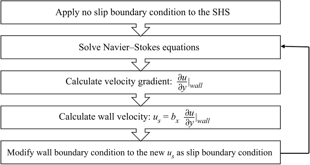
Figure 2. Flow chart of the simulation procedures for implementing slip velocity.
Simulations were conducted for five different inlet velocities for the RANS simulations, including 1.11, 1.25, 1.35 and 1.46 m s−1. Afterward, the simulation was continued with the DES and LES methods separately to obtain the transient flow simulation. A Courant number of 0.3 was considered for all simulations to determine the time step value. Simulations continued until the stationary condition was achieved (typically eight flow cycles). The convergence criterion of  ${10^{ - 6}}$ was considered for steady simulations, i.e. RANS model. Whereas for the DES/LES simulations, the solution was considered to be converged in each time step if the residuals of flow equations reach ${10^{ - 3}}$.
3. Results and discussion
In this section, the results for the flat and grooved SHSs are discussed. First, mesh verification is evaluated to ensure the appropriate element size. Then, the reliability of the utilized Navier slip condition will be examined by validating numerical results to the experimental data. Finally, the slip condition will be applied to the grooved SHS and the underlying physics of the turbulent flow discussed.
3.1 Mesh independency
The mesh independence analysis was first investigated to verify the performance and choice of numerical parameters. For the RANS simulations, to investigate the sensitivity of the numerical solution to the mesh size, three different meshes consisting of 4.5, 6 and 6.5 million cells were generated, and the variation of the wall shear stress and slip velocity was investigated. It was concluded that the difference in the average wall shear stress and slip velocity between the two latter meshes was no more than two per cent. We then chose 6 million cells to perform further simulations.
Moreover, the LES index of quality (LESIQ) proposed by Celik et al. was utilized to assess the LES mesh which is defined as  $\textrm{LESI}{\textrm{Q}_v} = 1/(1 + 0.05{[(\mu + {\mu _{sgs}})/\mu ]^{0.53}})$, in which $\mu $ and ${\mu _{sgs}}$ are fluid and SGS turbulent viscosities, respectively (Reference Celik, Cehreli and YavuzCelik, Cehreli, & Yavuz, 2005). The purpose of this parameter is to evaluate the proportion of total kinetic energy resolved by LES on each element. Accordingly, an LES computation can be judged to be well resolved when 80% of the turbulent kinetic energy is resolved, i.e. $\textrm{LESI}{\textrm{Q}_v} > 0.8$ (Reference Gousseau, Blocken and HeijstGousseau, Blocken, & Heijst, 2013). As shown in figure 3, the value of $\textrm{LESI}{\textrm{Q}_v}$ ranges between 0.897 and 0.952, which is acceptable for the LES simulation (Reference Celik, Cehreli and YavuzCelik, Cehreli, & Yavuz, 2005). Moreover, the value of dimensionless wall distance, ${y^ + }$, was calculated across the wall boundaries and is presented in table 1.

Figure 3. The LES index of quality contour for simulations in the middle plane along the channel flow, where SHS is located at the bottom.
3.2 Flat SHSs
Figure 4 shows the velocity contour along the channel, where the SHS is located at the bottom and the flow is in the positive x-direction. Different values of the slip velocity confirm that it is dependent on the local gradients of the flow field. Slight increases in the non-uniformity of the streamwise velocity fluctuation and turbulent kinetic energy were detected along the SHS surface. As illustrated in figure 4, Navier's slip boundary condition leads to inhomogeneous velocity fields on SHSs, enhancing turbulent structures. Enhanced vortical structures near the SHS can be observed from the comparison of figure 6(c,d) as well.

Figure 4. The LES result of the instantaneous velocity contour in channel flow where the SHS is located at the bottom. Four sections across the channel were created to visualize the velocity contour. The inhomogeneous velocity field on the SHS is due to the Navier slip boundary condition (Re = 9400)
3.2.1 Shear stress and slip velocity
The numerical results were compared with an experimental study by previous research (Reference Rowin and GhaemiRowin & Ghaemi, 2020) in which a two-dimensional particle image velocimetry (PIV) was used to measure the slip velocity and slip length, and near-wall Reynolds stresses were measured by using the three-dimensional particle track velocimetry method. Prior to demonstrating the near-wall behaviour of the SHS, the numerical results were validated using experimental data in terms of slip velocity, and smooth and superhydrophobic wall shear stresses. As shown in figure 5, in the presence of a slip velocity, the shear stress of the SHS was reduced compared with a no-slip surface. Overall, the DES and LES results correlated well with the experimental data. Similarly, the RANS results showed an acceptable accuracy, and therefore, all the simulation results were found to be within an acceptable error range. However, as mentioned by previous authors, RANS generally comes with primary shortcomings in terms of turbulence modelling. For instance, secondary flows induced by anisotropic turbulence cannot be precisely captured with this model (Reference Cauwenberge, Schietekat, Floré, Geem and MarinCauwenberge, Schietekat, Floré, Geem, & Marin, 2015). Moreover, the RANS model was unable to accurately account for the fluctuations of the flow field (Reference Salim, Ong and CheahSalim, Ong, & Cheah, 2011) which led to underpredict turbulent mixing (Reference Verma, Yadav, Nakod, Sharkey, Li and MeeksVerma et al., 2019) and, as a consequence, higher velocities and shear rates near the wall were derived. Hence, as expected, the RANS model demonstrated higher amounts of error with respect to the other turbulence models.

Figure 5. Comparison of numerical results with experimental data for wall shear stress of (a) a no-slip (smooth) surface and (b) an SHS. (c) Slip velocity for different inlet flow velocities.
3.2.2 Mean velocity profiles
Figure 6(a) demonstrates the mean velocity magnitude profiles of the LES models over the smooth surface and SHS for a Reynolds number of 9400. The mass flow rate was kept constant through the simulations, therefore the velocity across the channel slightly changed due to the slip velocity of the SHS. In figure 6(a), the alteration of the mean velocities by the SHS was clear, in contrast to the results of the smooth (no-slip) surface. The near-wall velocities over SHS shifted upward due to streamwise slip, which eventually affected the flow velocity pattern of the entire channel.

Figure 6. (a) Mean velocity magnitude profile at Re = 9400 for smooth (no-slip) and SHSs. An SHS is located at y = 0. (b) A comparison between vorticity magnitudes of ‘Smooth’ and ‘Superhydrophobic’ surface cases in the vicinity of the SHS zone. Contour and vector of velocity at the plane x = 0.9 m for (c) the smooth (no-slip) surface. (d) An SHS.
To be more clear, the vorticity magnitude near the wall is plotted in figure 6(b). The SHS caused more turbulent vorticity and fluctuation near the surface and resulted in enhancing the inner layer mixing in the vicinity of the SHS. Hence, the vorticity magnitude of the SHS is higher throughout the normal direction with respect to the no-slip surface. Figure 6(c,d) shows the contour and vector of velocity for the smooth and SHS at Reynolds number of 9400. The velocity magnitude incorporated a higher value adjacent to the SHS than that of the smooth surface.
Semi-logarithmic profiles of  ${u^ + }$ over the SHS for Reynolds numbers 6200 and 9400 are presented in figure 7. The DES and LES results are compared with the PIV measurements as well as the smooth, i.e. no-slip, surface profile (in logarithmic law). There was an upward shift of ${u^ + }$ for the SHS when compared with the logarithmic law, due to the slip velocity. The normalized mean streamwise velocity is, thus, defined as ${u^ + } = u/{u_\tau }$, where the frictional velocity $({u_\tau })$ is calculated from $\sqrt {{\tau _w}/\rho } $. Here, ${\tau _w}$ is calculated by averaging the shear stress value over the SHS. As shown in figure 7, our simulation code could successfully capture the velocity profile near the SHS. The velocity profile by DES can be regarded to be in the uncertainty range of the experimental results.

Figure 7. Semi-logarithmic profile of the mean streamwise velocity over the SHS at (a) Re = 6200, (b) Re = 9400.
3.2.3 High-order flow quantities
The high-order flow quantities such as statistical Reynolds stresses and the velocity fluctuations have been explored to further evaluate the influence of slip boundary conditions of SHS on the channel flow dynamics. The non-zero components of the Reynolds stress tensor,  $\langle {u_i}{u_j}\rangle $, adjacent to the SHS in slip boundary cases were calculated for the DES and LES simulations. The profiles were normalized by the lowest value of the inlet velocity throughout all the cases, i.e. 0.95 m s−1, and compared with experimental data (Reference Rowin and GhaemiRowin & Ghaemi, 2020). Subsequently, the LES results were in better correlation with experimental data in comparison with DES. Figure 8 compares the results of these two numerical approaches for a Reynolds number of 9400.

Figure 8. A comparison between LES and DES in terms of (a) streamwise, (b) wall-normal, (c) spanwise and (d) shear Reynolds stresses over the SHS.
Figure 9 compares the LES results of the components of the Reynolds stress tensor over the SHS for three Reynolds numbers of 6200, 8000 and 9400, to those of the experimental data. As expected, the Reynolds stresses increased with the increase of Reynolds number. With regards to the streamwise Reynolds stress, i.e.  $\langle {u^{\prime 2}}\rangle $, the maximum value shifted toward the wall with the increase of Reynolds number because of a thinner inner layer at higher velocities. Moreover, due to the small wall-normal and spanwise gradients of the velocity components the Reynolds stresses of these directions were one order of magnitude smaller than that of the streamwise Reynolds stress.

Figure 9. The LES results of (a) streamwise, (b) wall-normal, (c) spanwise and (d) shear Reynolds stresses over the SHS.
By increasing the Reynolds number, the near-wall velocities shifted upwards because of the streamwise slip velocity, as shown in figure 7. Similar behaviours were also observed on Reynolds stresses along the SHS, as illustrated in figure 9. Moreover, the streamwise Reynolds stresses in the outer layer were reduced continuously due to the decrease in the production of the streamwise turbulence. On the other hand, the wall-normal and spanwise Reynolds stresses and Reynolds shear stress increased due to the increased vortex transport term, which was correlated to the production of the near-wall vortices.
3.3 Superhydrophobic rectangular grooved surfaces
After we validated our simulation code on a flat SHS in comparison with the experimental results (Reference Rowin and GhaemiRowin & Ghaemi, 2020), we describe how we further extended our simulation code to the grooved surfaces with superhydrophobicity, which is expected to be more effective in drag reduction (Reference Ermagan and RafeeErmagan & Rafee, 2018) (Reference Fuaad and PrakashFuaad & Prakash, 2019). In conjunction with the SHS, the grooved surface achieves better drag reduction owing to the secondary vortex effect. Streamwise rectangular grooves were located across the SHS with the same geometry configuration for simulation. The width and depth of these grooves were 500 and 250 μm, respectively, corresponding to the width-to-depth ratio of 0.5, which has been reported to be the optimal value (Reference Soleimani and EckelsbSoleimani & Eckelsb, 2021).
We applied two boundary conditions for the grooved surface configuration, as shown in figure 10. For the first case, the grooved partitions were assumed to be filled with air and therefore the shear-free boundary condition was applied to them, and the rest were considered to have a slip velocity. For the second case, the slip velocity (Navier slip) was applied to the entire surface of the SHS. The simulations for the grooved surface were done at Reynolds numbers of 6200, 8000 and 9400. To achieve good precision in the grooved regions, fine grids were generated (figure 10). The hexahedron structured meshes were utilized with the aid of the blocking technique using the ICEM CFD package.

Figure 10. The boundary conditions for: (a) air-filled SHS (shear-free boundary condition), (b) the grooved SHS (Navier's slip boundary condition). All dimensions are in mm.
3.3.1 Shear stress and slip velocity
A comparison of simulation results for different surface configurations is presented in table 2. The drag reduction was calculated based on the shear stress defined as  $DR = \; (\tau _{wall}^0 - {\tau _{wall}})/\tau _{wall}^0$, where $\tau _{wall}^0$ and ${\tau _{wall}}$ are shear stresses measured on the smooth and superhydrophobic walls, respectively. The air-filled case experienced a higher drag reduction than the other scenarios. However, the assumption of air-filled grooves is revealed to be exaggerated, whereas the partially slipped (grooved SHS) case can be regarded as a more realistic representation of the model which experienced a drag reduction of 46% (12% more than a flat SHS).
Table 2. Drag reduction comparison between different surface morphologies for Reynolds number of 9400.

Moreover, the effect of changing the Reynolds number is presented in figure 11. The air-filled case incorporated higher slip velocities with respect to other scenarios even for the grooved SHS. This is due to the effect of the riblets’ sidewalls in decreasing velocity. However, the grooved SHS case demonstrated lower shear stress corresponding to the change of the vortical structures in the boundary layer. There will be further discussion on this topic in § 3.3.3.

Figure 11. Reynolds number dependence for the grooved SHS case of (a) slip velocity and (b) wall shear stress.
3.3.2 Mean velocity profiles
The streamwise velocity profiles of different surface configurations in the semi-logarithmic scale for Re = 9400 are shown in figure 12. In the viscous and buffer layers of the boundary layer, the velocity magnitude shifted upward for both air-filled and grooved SHSs in comparison with the flat SHS. Additionally, due to the shear-free condition in the air-filled model, the boundary experienced higher values of the slip velocity with respect to other cases.

Figure 12. Semi-logarithmic profile of the mean streamwise velocity over different SHS configurations for a Reynolds number of 9400.
3.3.3 Velocity fluctuations
In the following section, the high-order flow quantities including Reynolds stresses as well as turbulent structures are discussed in order to evaluate the effect of the surface grooves on the flow dynamics.
Reynolds stresses: the non-zero components of the Reynolds stress tensor for different surface configurations were compared to assess their contribution to turbulent structures. The grooved SHS demonstrated higher values of Reynolds stress with respect to other scenarios, as depicted in figure 13. As mentioned in § 3.2, on the flat SHS, the slip condition reduces the viscous drag force and enhances turbulence. Moreover, the riblets’ shape controls the vortical structures in the turbulent boundary layer, leading to less momentum transfer and shear stress. This grooved surface morphology enhances turbulent structures near the surface that contribute to the reduction of drag. Therefore, this effect causes more drag reduction in the grooved case over the flat case. As for the air-filled (shear-free) case, the underestimated shear stress may be attributed to the geometrical simplification. Hence, neglecting the effects of the grooves may lead to notable errors. The grooved surfaces significantly increased the intensity of the streamwise and spanwise turbulent fluctuations. Moreover, the peak of Reynolds stresses decreased and became closer to the SHS surface as for the grooved case.

Figure 13. Reynolds stress comparison for the flat, air-filled and grooved SHSs in terms of (a) streamwise, (b) wall-normal, (c) spanwise and (d) shear Reynolds stresses over the superhydrophobic region.
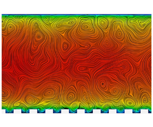
Turbulent structures: as emphasized by previous work (Reference Soleimani and EckelsbSoleimani & Eckelsb, 2021), surfaces with riblets alter the vortex structures in channel flows. The momentum of turbulent structures in the near-wall region is affected due to the existence of vortices in the riblets, and consequently, the flow field is altered in the spanwise direction. Principally, the visualization of coherent vortical structures can provide valuable insight into the flow field. Hence, to provide a better observation of the relationship between turbulence and drag reduction over the SHS, the representation of the vortical structures based on the line integral convolution (LIC) concept is depicted in figure 14. The LIC technique produces streaking patterns that follow the velocity vectors tangentially. More details of the implementation of this technique can be found in previous research on this (Reference Cabral and LeedomCabral & Leedom, 1993). Accordingly, velocity contours and streamlines for different cases are shown in figure 14. Both the grooved and air-filled models exhibit higher velocity magnitudes and vortices near the SHS boundary (at the bottom). The grooved SHS generated even more turbulent eddies near the SHS resulting in better flow interaction with respect to the flat SHS. The increased wall-normal and spanwise Reynolds stresses for the grooved SHS are attributed to the generation of near-wall vortices as well. Moreover, in the grooved SHS case, some tiny vortical structures were observed near the SHS, in particular, inside the grooves. This proves that more vortical structures exist in the grooved SHS, which cannot be truly captured by assuming an air-filled model.

Figure 14. The LIC illustration at the plane of x = 0.9 m for (a) flat SHS, (b) air-filled grooved surface and (c) grooved SHS.
The three-dimensionality of the flow dynamics was evaluated in terms of the Q-criterion, which is directly derived based on the second invariant of the velocity gradient tensor. The abundant multiscale vortices of the SHS were determined by the Q-criterion approach to present turbulent structures (Reference Krastev, Amati, Succi and FalcucciKrastev, Amati, Succi, & Falcucci, 2018; Reference Zhan, Li, Wai and HuZhan, Li, Wai, & Hu, 2019). In this method, the vortices were defined as areas where the vorticity magnitude is greater than the magnitude of the rate of strain with the following expression:
 \[Q = {1/2}(\|\varOmega\|^2 -\|S\|^2), \]
where Q > 0 represents the existence of a vortex. In (3.1), Ω is the vorticity tensor and S is the rate of strain.
Figure 15 shows the iso-surfaces of three-dimensional vortical structures for the flat SHS, air-filled and grooved SHS based on a normalized Q-criterion of 0.2. The vortical structures are elongated in the streamwise direction with a reduction in size near the wall boundaries (Reference Im and LeeIm & Lee, 2017). The density of vortical structures in the wall region is dependent on the hydrodynamics of the wall. As indicated in the top and side views of the flat SHS and air-filled cases, the density of the vortical structures increases for the latter case. As mentioned before, this corresponds to the reduction of shear stress and an increase in turbulence. Moreover, another turbulence initiative for the air-filled case is the alternative velocity boundary condition along the spanwise direction on the SHS boundary, which may contribute to the density of the vortical structures.

Figure 15. Contour of the instantaneous three-dimensional vortical structures for (a) flat SHS, (b) air-filled and (c) grooved SHS cases. The cross-section in the x–y direction shows the side view of vortical structure from the bottom of the channel, where the SHS is placed, to the top wall. The cross-section in the x–z direction shows the contour in the top view from the sidewall to the centreline.
By comparing the air-filled and grooved cases, the latter constitutes a higher density of vortical structures. The vortical structures in the air-filled case are mainly dependent on the shear-free boundary condition. However, the geometrical manipulation, as exists in the grooved SHS, generates more vortical structures than the simple shear-free boundary condition.
4. Conclusions
The SHS alters the symmetry, peak magnitude and location of Reynolds stresses, which implies the presence of a significant slip velocity and consequently a high amount of the shear stress reduction on the SHS. Previous research studies have shown the great potential of SHSs for drag reduction applications and have examined the near-wall behaviour in turbulent flows as well. The main purpose of this study was to shed light on the underlying mechanisms of turbulent structure alternations by considering the SHS. High- to intermediate-fidelity turbulent models including RANS, DES and LES were evaluated to explore the superhydrophobicity for wall-related turbulent statistics by utilizing Navier's slip boundary condition. The boundary condition was then developed and validated in terms of the shear stress, velocity and Reynolds stresses.
The focus of this research differs from previous investigations by addressing the modelling of the turbulent channel flow in three important aspects. First, the Navier slip boundary condition was considered for the walls of the SHS. The velocity magnitude on the SHS was then calculated in each time step resulting in a better understanding of near-wall behaviours. Second, simulations were performed in a broad range of Reynolds numbers and the effects of turbulent models and SHS configurations were assessed. Third, the present work compared the grooved SHS case with frequent modelling approaches in the literature including shear-free and slip boundary conditions.
From our simulations, we found that the RANS solver cannot capture flow structure near the SHS as accurately as the LES approach. In contrast, the DES and LES methods captured boundary layer phenomena with excellent agreement with the experimental data. In addition, the shear stress derived from LES was comparable to experiments. However, DES was not able to resolve Reynolds stresses precisely. Moreover, the slip condition causes the turbulent structures to move toward the SHS. The utilization of the LES model can truly predict some of the physics in turbulent wall-bounded flow on the SHS without the need for performing DNS.
Finally, the simulation was implemented to observe the near-wall behaviour in grooved surfaces to achieve further insight into the effects of the SHS on the drag. Flow patterns of the grooved SHS were compared with that of the flat air-filled assumption at a relatively high Reynolds number. The grooved SHS results showed a drag reduction of up to 48.9% over SHS. Furthermore, Reynolds stresses components were considerably higher for grooved SHS than that of the flat, leading to a more efficient reduction of the shear stress. The peak of Reynolds stresses increased and relocated closer to the SHS in the slip model with respect to the air-filled case. For future work, more comprehensive studies of other geometrical parameters are required to investigate the dependence of drag reduction on other factors such as different texture shapes and a range of pitch dimensions.
Supplementary material
Data is provided within the paper. For specific requests, please contact the corresponding author.
Funding Statement
This research was supported by grants from the National Science Foundation of China (grant no. 91952107).
Declaration of Interests
The authors declare no conflict of interest.
Author Contributions
A.S.: conceptualization, methodology, investigation, software, writing – original draft, review and editing, formal analysis. M.H.S.: supervision, review and editing. S.S.: methodology, software, review and editing. S.Y.: conceptualization, methodology, supervision, writing – review and editing, funding acquisition.


 Open access