


1. Introduction
Aviation is a critical mode of transportation in Alaska and is required to reach many areas within the state. However, a recent study covering the period of 2008–2017 has revealed that aircraft accidents occur in Alaska at a rate 2.35 times that of the rest of the United States (Sumwalt et al., Reference Sumwalt, Landsberg, Homendy, Graham and Chapman2020). Much of this is related to a combination of complex topography, the local climate, and a poor in-situ network of meteorological observations. Several aviation accidents are related to low horizontal visibility (e.g. fog) which can result in controlled flight into terrain (CFIT). To improve the relatively limited network of meteorological observations in Alaska, and thus the situational awareness of pilots and meteorologists, the Federal Aviation Administration (FAA) has deployed a network of over 300 weather camera sites to supplement existing METAR observation platforms and provide real-time imagery of current conditions across the state (https://weathercams.faa.gov/; Fig. 1.).

Figure 1. Locations of METAR (yellow +) and web camera (red circle) stations used in this study. Also shown is the 3 km RTMA Alaska domain (red outline).
The Real Time Mesoscale Analysis (RTMA), produced by the National Weather Service, provides high-resolution hourly analyses of surface sensible weather elements, which include 2 m temperature and moisture, 10 m winds, cloud ceiling, cloud cover, and visibility via a two-dimensional variational (2DVar) analysis procedure for the Contiguous United States, Alaska, Hawaii, Puerto Rico, and Guam (De Pondeca et al., Reference De Pondeca, Manikin, DiMego, Benjamin, Parrish, Purser, Wu, Horel, Myrick, Lin, Aune, Keyser, Colman, Mann and Vavra2011). Here we focus on only the visibility analyses associated with the RTMA 3-km Alaska domain. The RTMA system currently assimilates horizontal visibility observations only from conventional (i.e. METAR) observation networks, which are quite sparsely distributed relative to the size of Alaska. While the RTMA provides analyses of many surface sensible weather elements, such as 2 m temperature and 10 m winds, here we focus only on the visibility analysis. In this study we investigate the assimilation of horizontal visibility observations derived from the network of web cameras.
2. Methods
2.1 Experiment design
In this study we first must derive an estimate of the surface visibility from the web camera network. Surface visibility is defined as the greatest distance in a given direction at which it is just possible to see and identify with the unaided eye (Visibility, 2020). Visibility is estimated using an algorithm called Visibility Estimation through Image Analytics (VEIA), which is described later. Of the approximately 320 web camera observation sites, 154 of them are unique in that they are not co-located with existing METAR stations. This provides us with a set of observations that we can compare with METAR stations while also having several sites in areas that are currently under-sampled (e.g., Fig. 1). We first conduct simple comparisons of observations at co-located sites to ensure the technique is able to detect conditions similar to present instrumentation. Following comparison we test the impact of assimilating these new observations by conducting three experiments: 1) a simple comparison against the first guess background field input into the RTMA (GES), 2) the control (CTL) which only assimilates the conventional visibility observations from METAR, and 3) CAMERA which assimilates both the conventional and web camera-based estimate of visibility. No observations are withheld from the RTMA for the purposes of cross validation as it is instructive to assess the analysis under the context in which it is used, meaning all observations of sufficient quality are assimilated.
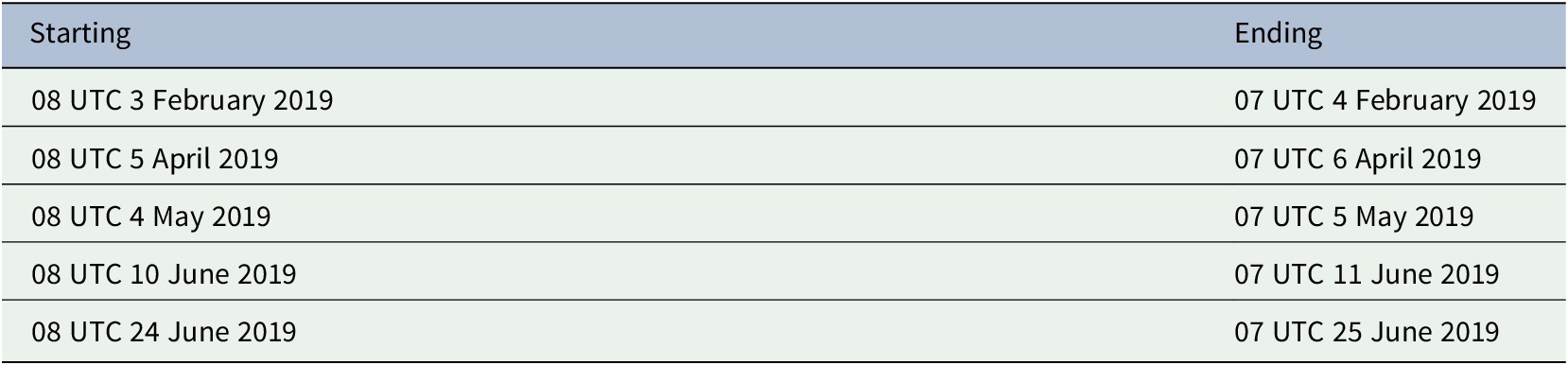
All tests and experiments are conducted with a set of 5 cases, each encompassing a 24-hr period, that were identified to be of interest based upon subjective examination of meteorological features and prevailing visibility conditions (Table 1).
Table 1. Periods during which experiments were conducted. The RTMA was run consecutively every hour during each period.
2.2 Estimating visibility from web camera data
The VEIA algorithm uses edge detection to estimate the visibility at the FAA network of camera sites. Each site consists of anywhere from one to four cameras, with most sites typically having four cameras to provide 360 $ {}^{\circ } $ coverage. The algorithm first estimates the visibility for each camera and then calculates a prevailing visibility for the site applying a weighted average to each camera based on sun position relative to the camera and other factors. The individual camera design is based upon four components; composite image generation, edge extraction and selection, measurement of edge strength ratio, and a translation of edge strength ratio into visibility (Fig. 2). The system ingests the color images and converts them to grey-scale for a Sobel-Feldman edge extraction (Sobel & Feldman, Reference Sobel and Feldman1968). The first component is saving a history of the last several days of clear camera images and processing them nightly into a composite image, which represents a clear-day reference image (i.e. unrestricted visibility). Any reduced-visibility images encountered are removed from the compositing process. The next component is edge extraction and selection. During this process, the Sobel-Feldman edge detection algorithm is applied to the composite image, followed by an edge selection technique to identify persistent reference edges, such as the horizon and fixed buildings. Next the algorithm estimates the visibility by comparing the ratio of the sum of the selected edges from a current camera image with the sum of the selected edges from the composite image. Finally, the edge ratios are correlated to a visibility distance using a linear model that was developed over years of experiments. For the visibility estimation to be successful, sufficient sunlight is needed to illuminate the surrounding area. Therefore, observations are not taken during overnight and low sun angle conditions (< 15 $ {}^{\circ } $ below the horizon). The VEIA algorithm also provides a measure of confidence in each visibility estimate that accounts for known limitations due to the number of available cameras, lighting from the sun, and the agreement between the available single-camera estimates.
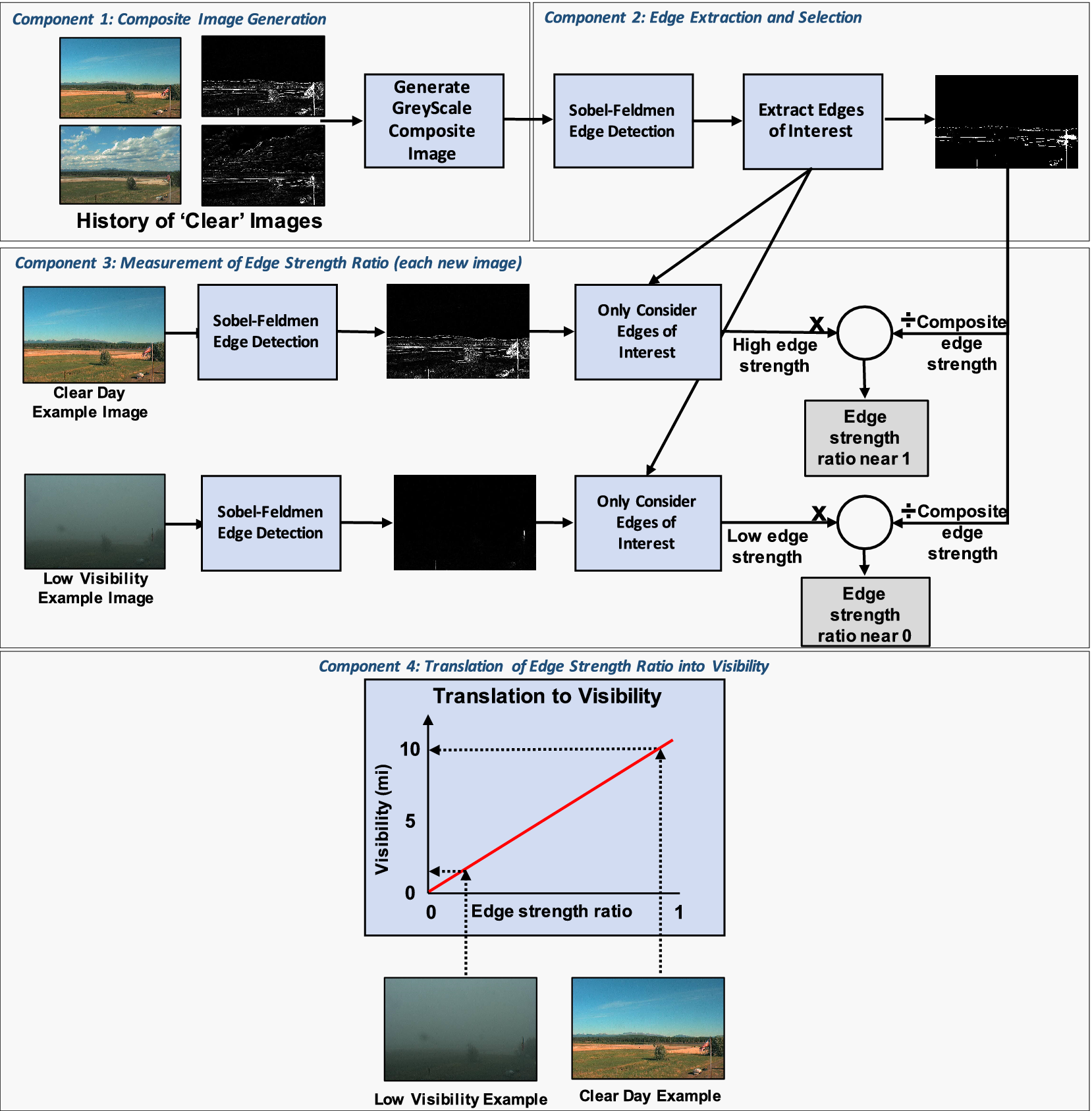
Figure 2. Flowchart depicting the components for estimating visibility from individual cameras.
2.3 The RTMA algorithm
The RTMA provides analyses for several areas across the United States and we focus here on the 3 km Alaska domain (Fig. 1). The RTMA’s 2DVar algorithm (De Pondeca et al., Reference De Pondeca, Manikin, DiMego, Benjamin, Parrish, Purser, Wu, Horel, Myrick, Lin, Aune, Keyser, Colman, Mann and Vavra2011) is based upon a Bayesian approach and minimizes a cost-function that measures the distance between the analysis and a background first guess forecast visibility from the High-Resolution Rapid Refresh system (https://rapidrefresh.noaa.gov/hrrr/) plus the distance between the observations and the simulated model equivalence, each weighted by their respective error covariance matrices. The optimal state, called the analysis, is the one that minimizes the cost function. The visibility observations are assimilated directly using a generalized nonlinear transformation function (Yang et al., Reference Yang, Purser, Carley, Pondeca, Zhu and Levine2020) to mitigate error associated with large cost-function gradient terms as well as with linearization of forward operators (Liu et al., Reference Liu, Xue and Kong2020). Observation error standard deviations for METAR and web camera-derived observations are specified to have a value of 2.61 dimensionless units. This value is based upon prior statistical analysis, single observation testing, and case study evaluation (not shown). Errors for the web camera data are adjusted based upon the provided, site-specific confidence index. The value for inflation follows a simple normal distribution, where low confidence yields a large error inflation (a maximum of 1.4x) and vice-versa (no inflation).
3. Results
3.1 Comparing web camera and METAR observations
METAR and web camera observations are stratified by FAA flight category (Table 2) at locations where the instruments are co-located (Fig. 1) for the 5 cases noted in Table 1. Co-located sites have a mean spacing of 0.8 km between camera and METAR instrument packages. For comparison, we consider only the camera observation that is reported within 10.2 minutes of the respective co-located METAR report time, corresponding to the closest possible temporal match. Fig. 3 shows that the web camera-derived visibilities correspond reasonably well with the METAR-observed LIFR conditions, but the distribution is wider under IFR conditions indicating a greater range of camera-derived visibilities relative to METAR. The MVFR category depicts a bimodal distribution of the camera-derived visibilities relative to METAR, with the highest density in the range of 2 miles and a second, lower density, near 10 miles. Such variability in agreement between camera-estimates and METAR observations in MVFR conditions may be related to the use of a linear translation function (Fig. 2) and suggests a potential need for recalibration under these conditions. VFR conditions, the most commonly observed event, have a peak in density at the 10 mile range which is accompanied by a long tail extending toward 1 mile. In general VFR conditions observed by METAR are consistent with camera estimates, but there may be considerable variability.
Table 2. Flight categories for visibility (statute miles), organized from least to most restrictive.
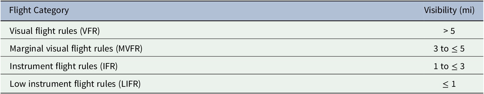
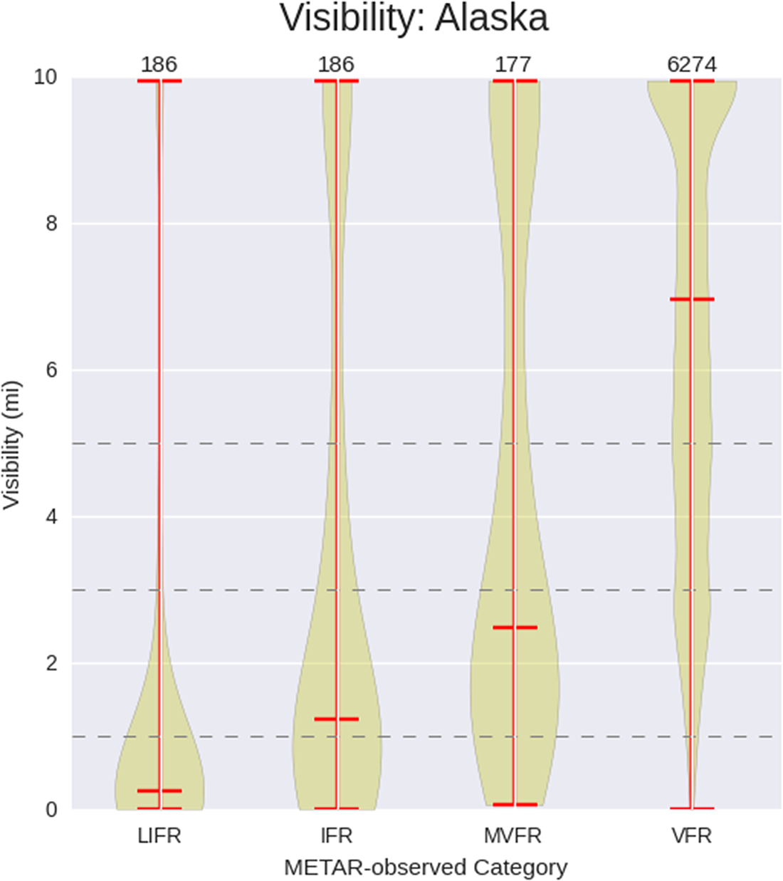
Figure 3. Violin plot showing sample distributions of the camera-derived visibility estimates stratified by METAR-observed flight category from Table 2 for all hours and dates listed in Table 1. The middle horizontal line in each violin depicts the median value while the top and bottom lines denote the maximum and minimum values, respectively. Each horizontal dashed line delineates transitions across FAA flight categories, bottom being LIFR, next area corresponding to IFR, followed by MVFR, and the top range corresponding to VFR. The number of METAR-observed events occurring within each category is annotated across the top of the figure. Violin plots are generated using a Gaussian Kernel Density Estimate with Scott’s rule for estimator bandwidth. The upper limit on visibility observations is capped at 10 miles to correspond with the upper threshold reported by METAR observations.
A recent study demonstrated that the RTMA performs well for less restrictive visibility conditions but for the most restrictive conditions of IFR and LIFR, it performs poorly and fails to properly characterize such events when they are observed approximately 50% of the time (Morris et al., Reference Morris, Carley, Colón, Gibbs, De Pondeca and Levine2020). Therefore additional observations that are capable of capturing IFR and LIFR events could prove beneficial in creating an analysis for aviation purposes, especially since these are the most restrictive, and thus impactful, thresholds for aviation.
3.2 Impact on analysis
Evaluation of the effectiveness of the assimilation is performed via the use of a performance diagram (Roebber, Reference Roebber2009), which summarizes four categorical verification scores derived from two-by-two contingency table statistics for dichotomous events (i.e. yes/no). We evaluate the fit of the analyses from all three tests (GES, CTL, and CAMERA) to METAR observations (Fig. 4) stratified by the FAA flight categories in Table 2. The probability of detection is increased, bias is improved (closer to unity), and critical success index is higher in CAMERA relative to CTL for LIFR and IFR conditions. However, the frequency of hits is slightly decreased, indicating an increase in instances of false alarms. For less restrictive categories, MVFR and VFR, we see a slight degradation in CAMERA relative to the CTL. This corroborates results noted in Fig. 3, which indicated that the camera-derived estimates could reasonably capture LIFR and IFR events but may have difficulty with events that are less restrictive.

Figure 4. Performance diagram comparing the first guess (GES; black), CONTROL (blue), and CAMERA (red) assimilating the web camera data. Statistics are calculated relative to METAR observations for the cases note in Table 1. Shapes indicate scores across four flight categories shown in Table 2, where a star corresponds to VFR conditions, triangle to MVFR or worse (i.e. more restrictive) conditions, circle to IFR or worse, and square to LIFR. The number of individual METAR sites at which the conditions are observed to have occurred is indicated in parenthesis. Probability of detection is shown on the ordinate, frequency of hits on the abscissa, the diagonal dashed lines are frequency bias (unbiased = 1), and grey shading corresponds to critical success index (CSI). For context, a symbol located in the upper-right corner would be a perfect score while a symbol in the lower-left would represent the worst possible score.
4. Conclusion
These results suggest the web camera data can supplement existing networks of visibility observations and improve the RTMA at the most restrictive, and impactful, categories of LIFR and IFR. However a slight degradation was noted at MVFR and VFR categories. Future work involves a recalibration of the VEIA translation function to reduce the number of incorrectly categorized VFR estimates as MVFR, thus improving the analysis at less restrictive thresholds, while maintaining the good performance at LIFR and IFR categories. Finally, this study suggests a potential to include a wider array of web camera networks, such as those for traffic and road condition monitoring. However, careful quality control and assessment of instrument siting are required to ensure meteorologically meaningful data can be obtained from these networks of opportunity.
Acknowledgments
The authors thank the two reviewers for their constructive comments on this manuscript. Haixia Liu, Eric Rogers, and Danny Sims are thanked for their helpful reviews of an earlier version of this manuscript. The authors acknowledge the high performance computing resources provided by the NOAA Research and Development High Performance Computing Program that supported this work. The scientific results and conclusions, as well as any views or opinions expressed herein, are those of the authors and do not necessarily reflect the views of NOAA or the Department of Commerce.
Author Contributions
J. R. Carley, M. Matthews, M. S. F. V. De Pondeca, and R. Yang designed the study. M. Matthews developed the web camera visibility estimate algorithm and provided the associated data. R. Yang performed the experiments. M. T. Morris performed analysis. J. R. Carley wrote the manuscript and managed the project. J. Colavito provided oversight and also managed the project.
Funding Information
FAA Disclaimer: This material is based upon work supported by the Federal Aviation Administration under Air Force Contract No. FA8702–15-D-0001 and Federal Aviation Administration Contract No. DTFACT-17-X-80002. Any opinions, findings, conclusions or recommendations expressed in this material are those of the author(s) and do not necessarily reflect the views of the Federal Aviation Administration.
Data Availability Statement
Web camera imagery is available at https://weathercams.faa.gov/. METAR observations are available from the National Center for Environmental Intelligence at https://www.ncdc.noaa.gov/has/HAS.DsSelect.
Conflict of Interest
The authors have no conflicts of interest to declare.


 Open access
Comments
Comments to the Author: 1) The following statement is vague. Can you provide an indication whether this is a critical source of potential error? “the edge ratios are correlated to a visibility distance using a linear model that was developed over years of experiments.”
2) Can you comment about some incorrect cases (camera VFR when METAR not, etc.). You could show a couple images and corresponding METAR observations to illustrate misclassification?
3) You might add a comment in the Conclusion that other sources of visibility are now available that could be used in future versions of the RTMA, including from road weather sensors that report visibility as well as estimates from thousands of road weather cameras that are distributed to NCEP I believe via the National Mesonet Program. However, the errors associated with those estimates are likely higher than from METAR sensors.