


Introduction
The current approximately 110 million population of Ethiopia is projected to reach 180 million by 2050 (Bekele and Lakew, Reference Bekele and Lakew2014; UNDESA, 2017). This requires an increase in huge tons of annual cereal and meat production to meet the nutritional and food security needs of the increasing population (FAO, 2017). This situation is worsened by the fact that over 60% of the farming households in the country operate on small plots averaging less than 1 ha (e.g. CSA, 2015; Rahmato, Reference Rahmato1994) and are fragmented with significant operational challenges (Zewdie and Tamene, Reference Zewdie and Tamene2020). Because of limited cultivable land for expansion, the efficiency of agricultural production on currently cultivated land should increase substantially to feed the growing population. This should be achieved without compromising ecological integrity and environmental sustainability. To realise this, resources should be targeted in a rational way to the production systems that have the highest potential to achieve the triple wins of poverty reduction, environmental protection and food security (Herrero et al., Reference Herrero, Notenbaert, Thornton, Pfeifer, Silvestri, Omolo and Quiros2014).
One of the key constraints to enhance food security and increase the overall resilience of smallholders in developing regions is a lack of informed decision making due to a combination of factors such as lack of locally relevant information, conducive institutional structure and policy issues (Aryeetey et al., Reference Aryeetey, Holdsworth, Taljaard, Hounkpatin, Colecraft, Lachat, Nago, Hailu, Kolsteren and Verstraeten2017; Covic and Hendriks, Reference Covic and Hendriks2016; Holdsworth et al., Reference Holdsworth, Aryeetey, Jerling, Taljaard, Nago, Colecraft, Lachat, Kolsteren, Hailu and Verstraeten2016; Shroff et al., 2015). The major bottleneck that aggravates the impacts of these constraints is the lack of adequate data at the appropriate resolution, desired frequency, required quality and quantity to deploy data-driven knowledge-based decisions (Donatien, Reference Donatien2016). For example, the lack of site-specific information about the topographic settings of farms, the status of soils, weather conditions and the nutrient requirements of crops undermines effective targeting of technologies to areas where they perform better to improve productivity.
As a result of the lack of data-driven and tailored decisions, farmers are provided with blanket recommendations of technologies and management practices despite considerable differences in their farming systems in terms of environmental conditions, landscape positions, soil characteristics, crop diseases, weeds infestation and water availability. This approach ignores the need to match ‘farming conditions’ with technology requirements and entails the need to shift from a ‘one-size-fits-all’ strategy to providing tailored recommendations based on location-specific characteristics, constraints and potentials. Therefore, in regions where there are heterogeneous farming systems, classification of sites into uniform units is a crucial step to develop location-specific recommendations and thereby improve agricultural productivity and food security (Penghui et al. Reference Penghui, Manchun and Liang2020; Pennock et al., 1994).
Classification of landscapes into relatively homogenous units is done by creating uniform territories with regular and typical occurrence of interrelated combinations of geological composition, landforms, surface and ground waters, microclimates and soil types (Salecker et al., Reference Salecker, Dislich, Wiegand, Meyer and Péer2019). By matching the specifications of a given development strategy with spatially referenced similar units, it is possible to delineate geographical areas where the strategy is likely to be successful and has a positive impact (Notenbaert et al., Reference Notenbaert, Pfeifer, Silvestri and Herrero2017). This will not only enable targeting technologies to areas where they perform better but also facilitates scaling options across wide areas (Herrero et al., Reference Herrero, Notenbaert, Thornton, Pfeifer, Silvestri, Omolo and Quiros2014; Notenbaert et al., 2013). In agriculture, the assumption is that strategies are likely to have similar response in areas that fall within the same recommendation domain. Thus, specific types of development policies, investments and livelihood options, and technologies are likely to result in a desirable effect and be adopted if they are targeted based on a recommendation domain.
The past few decades have seen widespread availability of spatial data and the advancement of robust modelling algorithms. Such developments are creating unique opportunities for optimisation of natural resource management, enhancing economic development and helping alleviate poverty on the basis of recommendation domains (Akıncı et al., Reference Akıncı, Özalp and Turgut2013; Elsheikh et al., Reference Elsheikh, Shariff, Amiri, Ahmad, Balasundram and Soom2013; Freeman et al., Reference Freeman, Noenbaert, Herrero, Thornton and Wood2008; Herrero et al., Reference Herrero, Notenbaert, Thornton, Pfeifer, Silvestri, Omolo and Quiros2014; Hyman et al., Reference Hyman, Hodson and Jones2013; Notenbaert et al., Reference Notenbaert, Pfeifer, Silvestri and Herrero2017, Reference Notenbaert, Herrero, De Groote, You, Gonzalez-Estrada and Blummel2013; Omamo et al., Reference Omamo, Diao, Wood, Chamberlin, You, Benin, Wood-Sichra and Tatwangire2006). Different approaches have been used to create environmental units where similar processes prevail, similar recommendations can be made and similar responses can be expected. In the agricultural sector, there are several efforts to define areas of high similarity. Examples include the development of agro-ecological zones (AEZ) (e.g. FAO, 1981; Fischer and Antonie, Reference Fischer and Antonie1994; IIASA/FAO, 2012), farming systems (e.g. Amede et al., Reference Amede, Auricht, Boffa, Dixon, Mallawaarachchi, Rukuni and Teklewold Deneke2017; Dixon et al., Reference Dixon, Gibbon and Gulliver2001; Rizzo et al., Reference Rizzo, Marraccini, Lardon, Rapey, Debolini, Benoît and Thenail2013), recommendation domains (e.g. Notenbaert et al., Reference Notenbaert, Herrero, De Groote, You, Gonzalez-Estrada and Blummel2013; Omamo et al., Reference Omamo, Diao, Wood, Chamberlin, You, Benin, Wood-Sichra and Tatwangire2006; Tesfaye et al., Reference Tesfaye, Jaleta, Jena and Mutenje2015) and topographic position (e.g. Amede et al., Reference Amede, Gashaw, Legesse, Tamene, Mekonen, Thorne and Schultz2020; Gerçek, Reference Gerçek2017; Gerçek et al., Reference Gerçek, Toprak and Strobl2011). Recently, Muthoni et al. (Reference Muthoni, Guo, Bekunda, Sseguya, Kizito, Baijukya and Hoeschle-Zeledon2017) used geospatial analysis and clustering techniques to delineate relatively similar clusters for scaling improved crop varieties and good agronomic practices in Tanzania. In addition, Khoroshev (Reference Khoroshev2020) developed a framework aimed at considering geographical context, matter flows and dynamic processes in developing ecological networks and identifying sites for various land use types as well as for choosing appropriate technologies.
Developing procedures to automatically classify landscapes into spatial entities or clusters can be essential to defining effective management units for precision farming and for scaling site-specific recommendations (Penghui et al., Reference Penghui, Manchun and Liang2020). There are, however, no standard frameworks designed to generate similar response units (SRUs) using big data and machine learning approaches. The aim of this study is, therefore, to develop an operational framework to define ‘SRUs’ or management zones within which similar technologies and management interventions can be recommended. We outlined a framework and approaches, with reproducible workflow and tool piloted for Ethiopia.
Approach and Methodologies
Study area
The SRU-mapping exercise is piloted in Ethiopia, which is a country with very heterogeneous landscapes (Figure 1), diverse AEZ and different farming systems. The country’s elevation ranges from 116 m below sea level to over 4600 m asl and comprises more than 30 AEZs. Generally, AEZs are defined through the combination of temperature, precipitation and elevation parameters focusing on the climatic and edaphic requirements of crops and on the management systems under which the crops are grown (FAO, 1996). Agriculture is the dominant means of livelihoods in Ethiopia supporting over 80% of the population. The Ethiopian highlands (over 1500 m asl) support the majority of the population, and this is also the part of the country where crop production dominates. Still traditional farming dominates and its transformation will be needed for enhancing the quality of life and improving food security. Owing to the country’s heterogeneity and diversity of agro-climatic and farming systems, it will be essential to ensure that appropriate options/technologies are targeted to locations with specific characteristics.

Figure 1. Topography of parts of Ethiopia revealing complexity and diversity.
Data and data sources
Integrating key variables is crucial for the zonation of target areas into similar management units. This study uses relevant covariates (Table 1) to develop SRUs that will have similar responses to agricultural technologies such as integrated soil fertility management and climate-smart agriculture. The major factors that determine agricultural systems and productivity are topography, climate, soil and associated derivatives. These are thus the key covariates used to derive SRUs.
Table 1. Key landscapes elements/variables used to drive similar response units
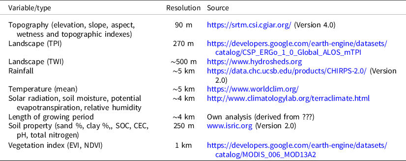
Topography and its derivatives (e.g. slope, aspect, wetness index and topographic index) determine landscape processes such as material flow as well as associated agricultural and landscape practices. Topography is the dominant factor in controlling the flow and accumulation of water, energy and matter in Ethiopian landscapes. It also affects the development and properties of soils and off-site environmental conditions (e.g. soil moisture, organic carbon, mineral-forming elements, etc.) in different ways. In this study, the 90 m SRTM digital elevation model was used to derive key terrain variables.
Climatic conditions such as temperature, rainfall, humidity, evaporation and their variabilities have important implications on determining the success of developed plans and interventions. Knowledge of localised climatic conditions (weather) and variability across space and time is thus critical to designing targeting options. The 5 km resolution CHIRIPS data set (Funk et al., Reference Funk, Peterson, Landsfeld, Pedreros, Verdin, Rowland, Romero, Husak, Michaelsen and Verdin2014) was used to represent rainfall and temperature conditions in the country; average and dekadal data sets were used to capture spatio-temporal and seasonal dynamics. Temperature was derived from 5 km WORLDCLIM data set (Fick and Hijmans, Reference Fick and Hijmans2017). The 4 km TERRACLIME (Abatzoglou et al., Reference Abatzoglou, Dobrowski, Parks and Hegewisch2018) data were used to represent solar radiation, soil moisture and potential evapotranspiration as input variables for clustering. A ‘climate derivative’ called the length of the growing period (LGP), which represents overall suitability for crops and vegetation, has also been derived. It is one of the crucial components for the agricultural domain as it not only considers both rainfall and temperature dynamics but also includes other important features such as soil moisture and potential evapotranspiration.
Soil dictates the types of farming systems that can function within a defined geographical unit and the associated management options. The amount and type of input to be applied for agricultural purposes, for example, are dictated by the properties of the soil and its health. Thus, soil is the predominant organising unit related to fertiliser and agronomic advisories. Knowledge of soil type and key soil properties is essential to defining environmental conditions and their overall suitability. In this study, soil texture, soil organic carbon (SOC), pH, cation exchange capacity, total nitrogen and proportion of sand and clay were used for the clustering exercise. Gridded layers for soil chemical properties with a resolution of 250 m were downloaded from the World Soil Information database (Poggio et al., Reference Poggio, de Sousa, Batjes, Heuvelink, Kempen, Ribeiro and Rossiter2021). The weighted average value of topsoil (0–30 cm) was used as it represents the average effective rooting depth of major crops.
Vegetation indexes are useful for characterising crop health and the potential capacity of the land to sustain vegetation. The normalised difference vegetation index (NDVI) and the enhanced vegetation index (EVI) are two vegetation indexes commonly used to monitor vegetation states and processes and are included in this framework. These two variables were used in the clustering exercise of this study.
Overall, 16 variable input layers were prepared for the clustering analysis in this study (Table 1). The key data-processing steps are presented in the following sections.
Data pre-processing
Figure 2 shows the major data-processing steps used in this study. All the data sets from global and/or regional sources were clipped based on the Ethiopian boundary. Because the different data sets have varied spatial resolutions, it was necessary to adjust to a common scale. In order to maintain the details of topographic (90 m) and soil-related information (250 m), and considering that climate variables will not significantly change over short distances, all the other data sets were resampled to 1 km resolution using the weighted average resampling method.
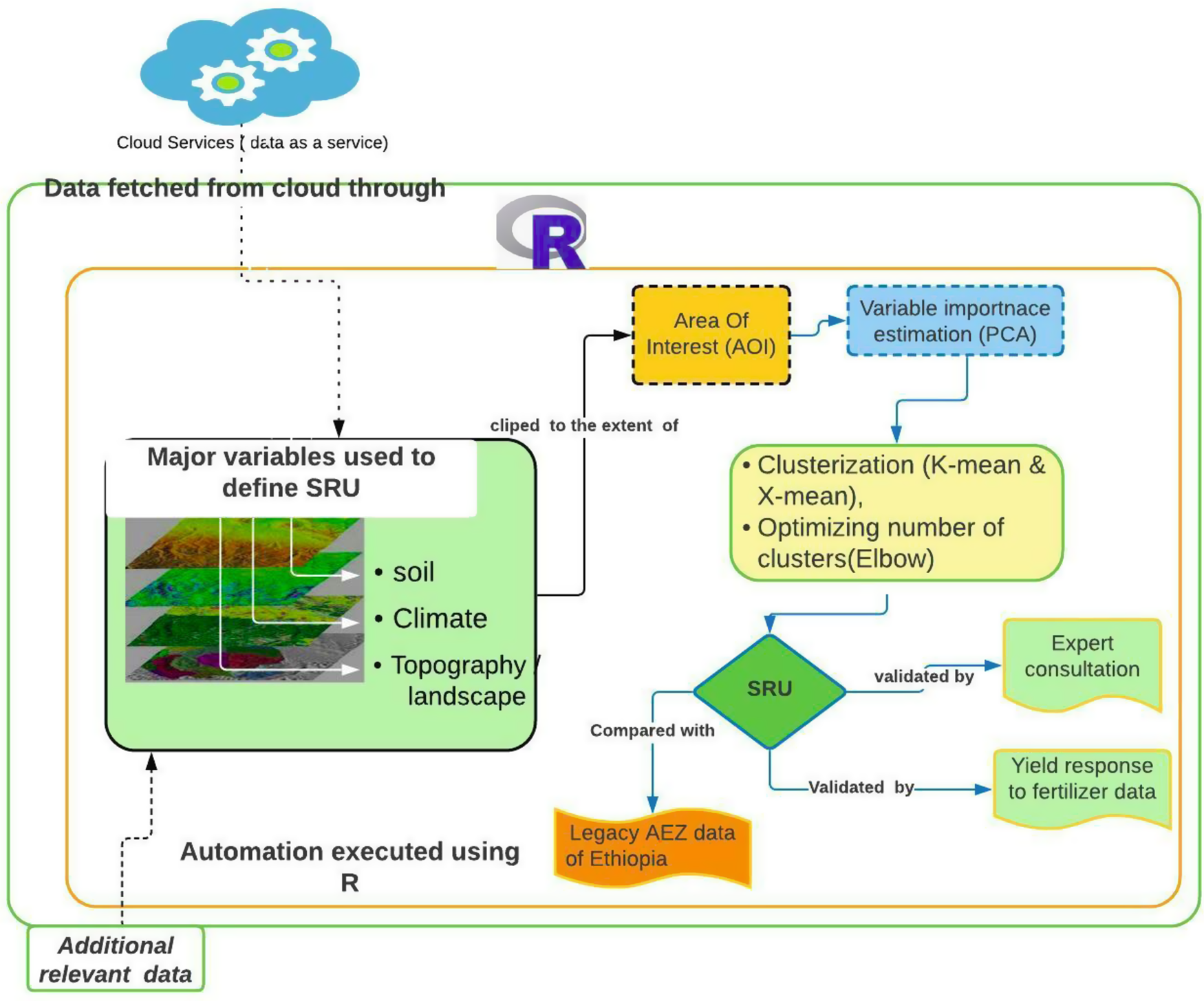
Figure 2. Flowchart showing the automation of SRU mapping.
To make a comparable (and avoid spurious) impact of variables with larger ranges of values, it was necessary to normalise data sets (Abbott, Reference Abbott2014). In this study, data sets from various ranges to a common range (0–1) were normalised using a min-max scaling procedure.
Variable importance was used to assess how effectively a variable can differentiate between clusters and determine whether to include it in the analysis. Fowlkes et al. (Reference Fowlkes, Gnanadesikan and Kettenring1988) developed a variable selection method that focuses on a reduced variable space to make the model create new clusters parsimoniously. In this study, a principal component analysis (PCA) was used to reduce the data dimension and maintain the important variables by excluding those which carry redundant information. PCA axes with eigenvalues greater than 1 were retained to ensure that only PCA axes with a significant contribution are used for further analysis (Kaiser and Rice, Reference Kaiser and Rice1974). Further, the quality of representation of the variables was analysed using the Cos2 indicator represented in a factor map. Cos2 represents the gradient of quality to highlight the most important variables in explaining the variations retained by the principal components (Kassambara, Reference Kassambara2016). The factor map help to visualise the cluster of correlated variables in groups (ibid.). Finally, we used moving window variance over a 10 km radius to calculate the spatial variance of each pixel for the final list of covariates.
Clustering to define SRUs
The SRU exercise targets partitioning the heterogeneous environment into similar units where similar processes prevail and similar interventions can be made. Clustering is an approach that involves classifying data points into a specific group based on the premise that data points that are in the same group/cluster would have similar properties and/or features, whereas data points in different groups would have highly dissimilar properties and/or features. The aim is to cluster areas in a manner that maximises within-group similarity with maximising between-groups dissimilarity, thus minimising the total intra-cluster variation or total within-cluster sum of squares (WSS) (Goswami et al., Reference Goswami, Chatterjee and Prasad2014). The total WSS measures the compactness of the clustering whereby ideal clusters should be compact, well-separated and stable (Brock et al., Reference Brock, Pihur, Datta and Datta2008). The point where the difference with the previous number of clusters flattens out represents the optimal number of clusters as determined by the elbow method (Kaufman and Rousseeuw, 1990).
One of the commonly used spatial clustering algorithms is the K-means (Hot and Popović-Bugarin, 2016; Jain et al., Reference Jain, Duin and Mao2000; Rahmani et al., Reference Rahmani, Pal and Arora2014; Shukla et al., Reference Shukla, Agrawal, Sharma, Chaudhari and Shukla2020). K-means is generally simple to implement and can be used with large datasets. The K-means is, however, not suited for use at a large scale due to the time it requires to give results when used for large areas and many covariates. In addition, it demands users to predefine the number of clusters to be produced. As a result, the X-means clustering method (Pelleg and Moore, Reference Pelleg and Moore2000) from the WEKA package (Beckham et al., Reference Beckham, Hall and Frank2016) has been developed as an extension of K-means to provide a more independent, unsupervised classification with improved computational efficiency, avoiding under parameterisation. Using X-means removes the necessity of a pre-set number of clusters from the user supporting the future developments of the approach developed in this study. The X-means approach is made efficient by replacing the need for K-means to compute the distance between every point to every centroid by recursive splitting of every cluster. It uses information criteria such as Bayesian information criterion (BIC) to select a model over another and whether the split at a centroid could be kept or not. The global BIC is used to define the final number of clusters. In this study, we used the X-means clustering method to group areas into similar or homogeneous zones within which similar recommendations can be made without requiring the need to predefine the number of clusters.
During the clustering exercise, all the variables (weather continues or categorical) were ingested into the classification algorithms, without any modification/creation of classes after normalisation. A moving window approach was used during classification to make the importance of the variables area/site specific.
Assessing the performances of clustering
To assess the results of the clustering algorithms, we have used qualitative and quantitative approaches. First, expert consultation has been used to gain an overall sense of the clustering results vis-à-vis expert knowledge and experiences of different geographical areas. At a one-day workshop, experts in soils, agronomy and geospatial analyses discussed the approaches used and corresponding clustering results. The maps were visualised on screen and printed in large colour prints to enable experts explore the results across the country. The second approach compared the distribution of standard deviation of optimal crop response to fertiliser application between the existing AEZ and the SRUs with the same number of classes. For this exercise, 3 commonly used AEZ maps categorised in 7 moisture belts and 15 AEZ (Hurni, Reference Hurni1998) and 33 zones (MoA, 2005) were selected. Corresponding SRUs with similar number of classes (7, 15 and 33) were then generated for ‘one-to-one comparison’’ Maintaining the same level of granularity (number of classes) between the SRUs and AEZs, we compared within standard deviation between the two at a national scale. In this case, the assumption is that because the ‘classes’ are a result of homogeneous factors, they are expected to respond similarly to interventions. The expectation is that there will be less variation (indicated by standard deviation) in the crop response to nutrient added within similar classes than between different classes. If the standard deviation of the optimal fertiliser rate for SRU is smaller than AEZ for the same level of classes, the SRU approach of generating agriculturally homogeneous units is considered more appropriate. The optimal fertiliser recommendation used for this purpose is collated from many trial data sets (Tamene et al., Reference Tamene, Amede, Kihara, Tibebe and Schulz2017) and analysed as outlined in Abera et al. (submitted).
Automation and tool development
One of the main aims of the study is to develop a scalable framework/system to delineate SRUs for different agronomic purposes. To build a generic system, the approach should primarily use globally available geospatial data sourced from the cloud with the flexibility for users to upload their own additional layers. The tool should also be designed to provide different options of clustering methods such as partitioning, distribution-based, hierarchical and fuzzy methods. The classification algorithms should also be designed to be scalable to run analysis for target areas of different spatial extent. The framework and tool developed in this study will thus enable the access of data from the cloud, and running clustering for a defined geographical area of interest using various approaches delineating similar zones. It also provides flexibility for user submit their own data to use solely for clustering and/or integrate with data derived from the cloud. The whole process is automated in an R programming environment and piloted for Ethiopia using commonly available geospatial data.
Results and Discussion
Variable selection for clustering
Figure 3 depicts the eigenvalues, variances and cumulative variances for the PCA analysis. The results show that the total cumulative variance percent of the three dimensions explained more than 80% of the variance. The first dimension explained 60% of the variance, whereas the second and third dimensions explained about 15% and 7%, respectively. Beyond the third dimension, variability lessens and the amount of new information that is carried diminishes. As a result, the first three dimensions were selected for further cluster analysis.
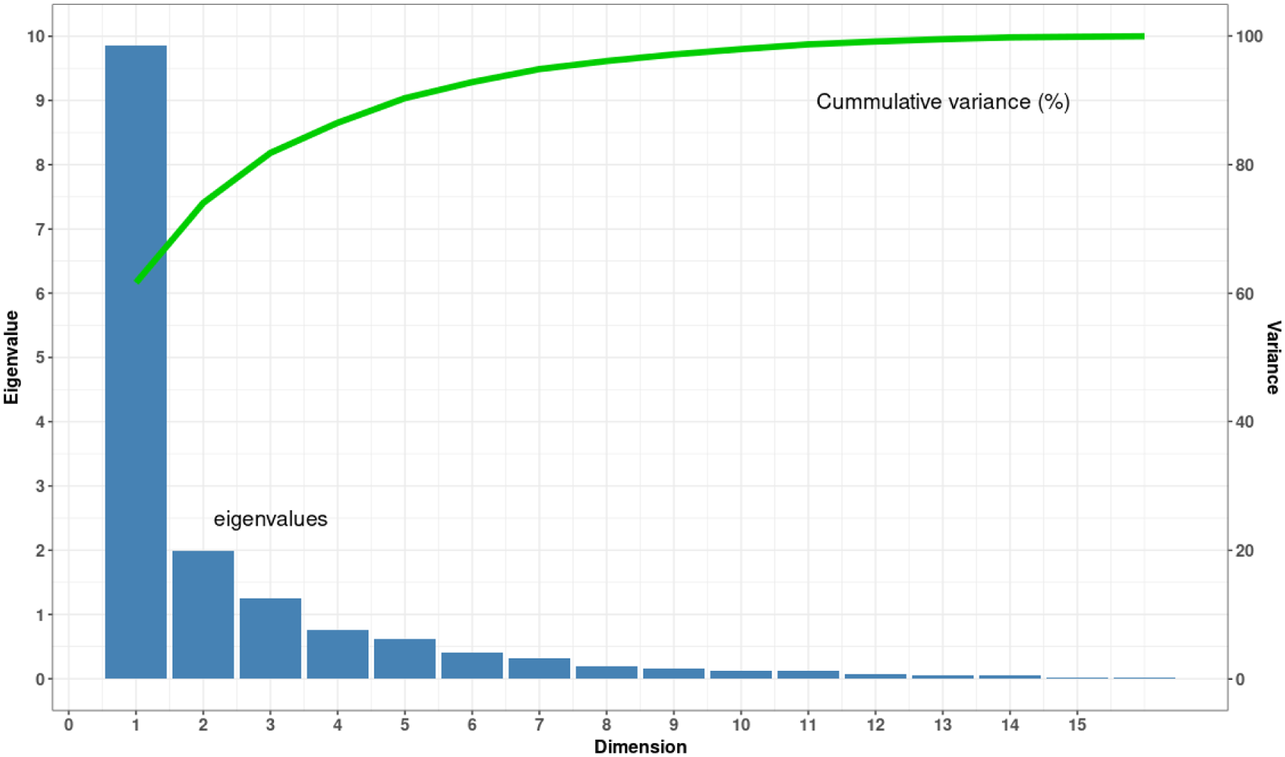
Figure 3. Eigenvalues, variance and cumulative variance of the PCA analysis.
Figure 4 shows the quality of representation of the variables on the factor map analysed using the Cos2 indicator. Generally, well-represented variables by the principal components are positioned close to the circumference of the correlation circle, whereas the less represented ones are located close to the centre of the circle. In this case, all the variables except slope are well represented by the principal components. Figure 4 also shows that the distances of the variables from the origin in all covariates are high, indicating that most of these variables are useful for cluster analysis. Accordingly, most of the variables such as precipitation, total N, SOC, LGP, NDVI, EVI, PET, elevation, solar radiation and soil moisture contributed to the clustering analyses (depicted in the correlation map of Figure 4).
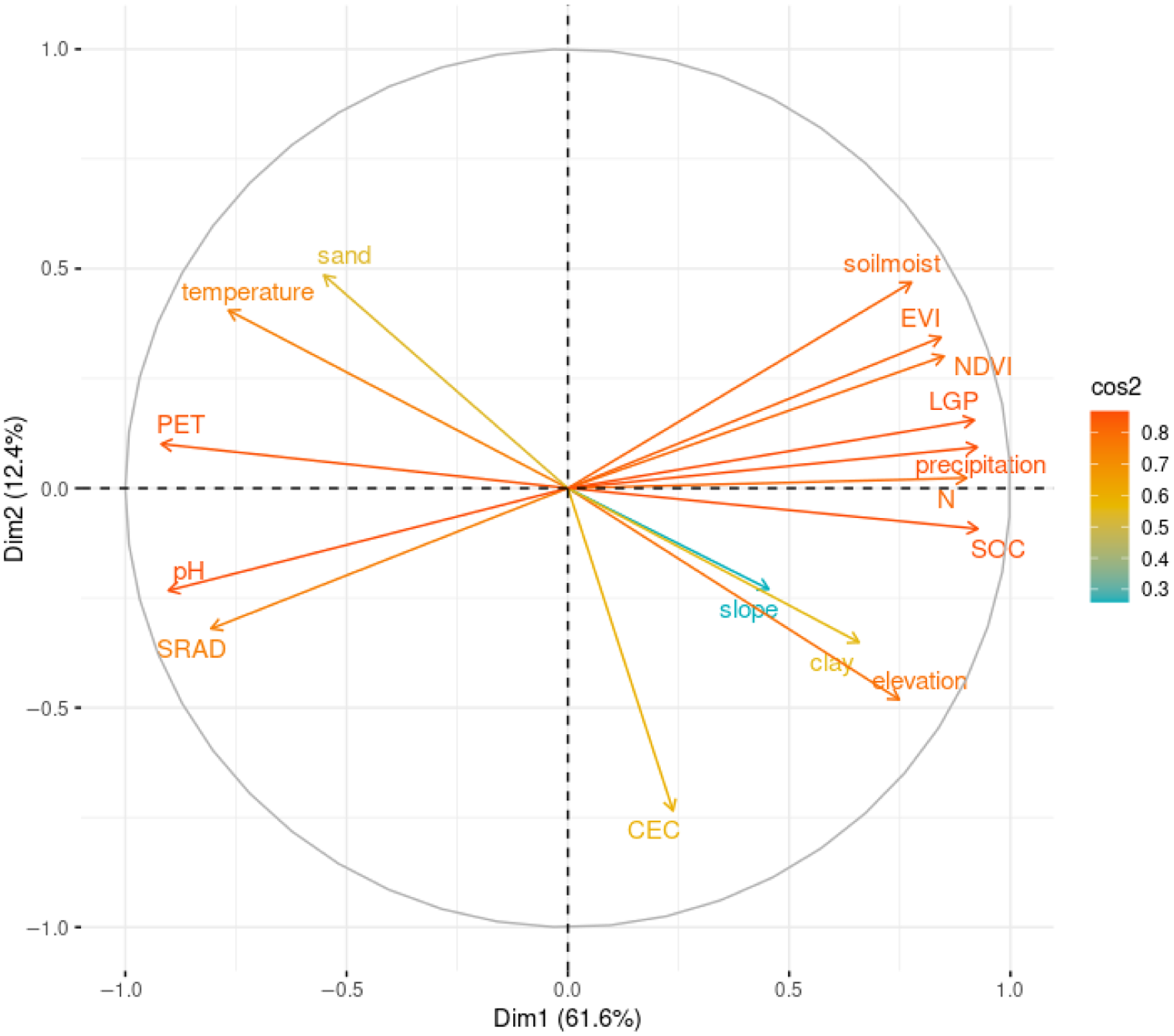
Figure 4. The representation quality of variables in the correlation plot.
The optimum number of clusters and SRUs
The K-means clustering result in Figure 5a shows the output of the WSS for the computation of 1–150 clusters. This visual representation is typically referred to as the ‘elbow method’ and allows the user to identify an appropriate number of clusters for an unsupervised classification exercise (Chiang and Mirkin, Reference Chiang and Mirkin2010). Though there is no straightforward ‘rule’ to determine which number of clusters can best perform, the general recommendation is to consider the position where the elbow tends to plateau compared with the other number of clusters (Jain et al., Reference Jain, Duin and Mao2000; Khan and Mohamudally, 2020). In Figure 5a, it is possible to identify the position(s) where the WSS of the clusters tends to flatten out. On the basis of the distinct elbows, three example clusters (with 9, 30 and 53 classes) can be distinguished in this study (Figure 5a). The corresponding spatial SRUs for the above three classes are shown in Figure 5b.
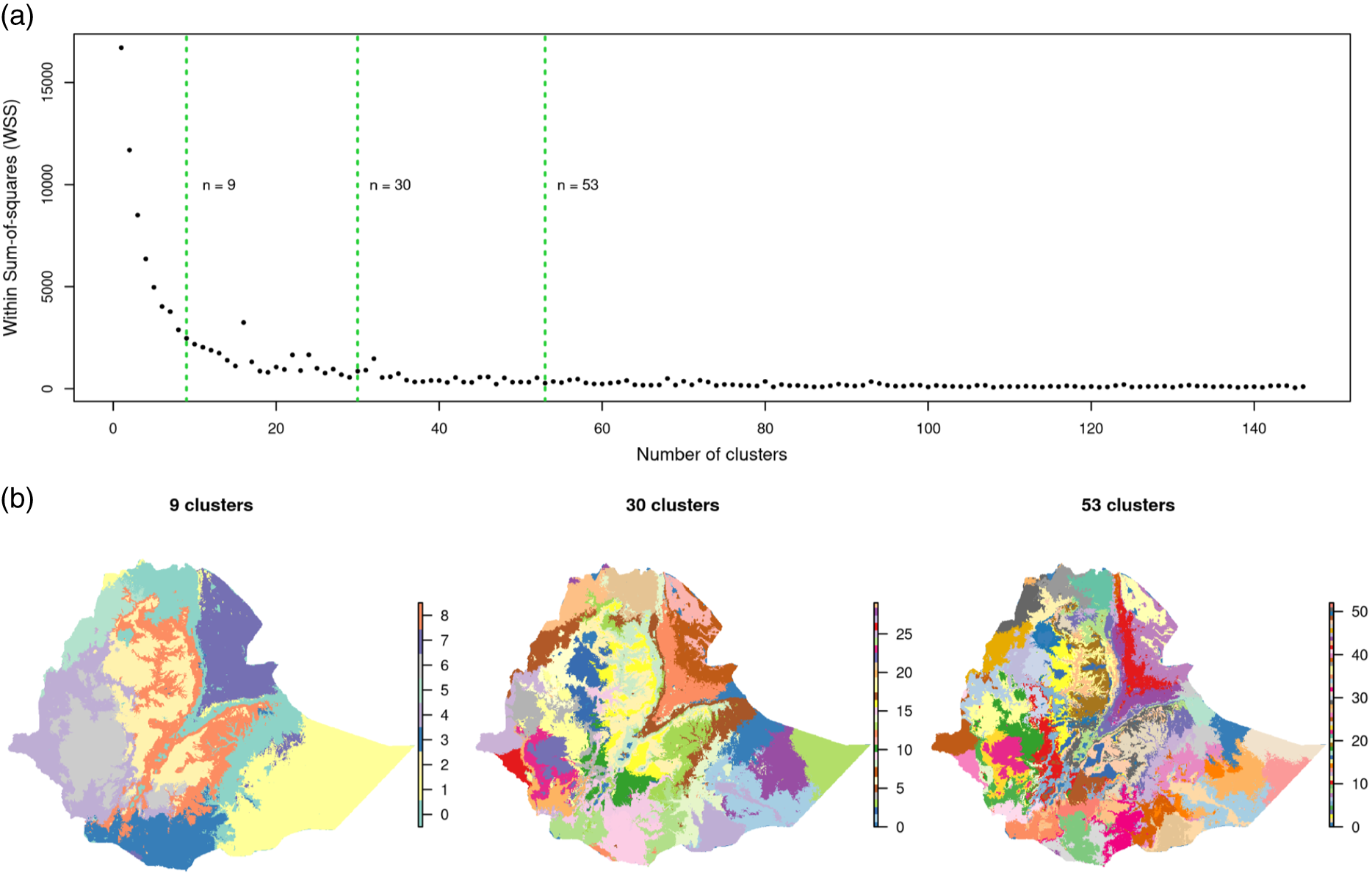
Figure 5. (a) Number of clusters using the elbow method in K-means clustering and (b) examples of clusters (SRUs) with three different number of classes.
The level of homogeneity of clusters needed can vary with the specific applications, and each of the maps shown in Figure 5b can be recommended for different applications. When considering macro-granular partitioning, it is possible to use fewer classes compared with applying for detailed process understanding and recommendation. In this example, SRU 9 (Figure 5b) can be used for applications/advisories that do not require detailed site specificity, such as identifying farming systems where detailed studies can be conducted. In this case, for instance, the lowlands like most parts of Somalia and the Afar region represent one unit each. The south-western highland forested area came out to be another separate unit (Figure 5b). When the number of clusters increases with the desire to obtain more detailed and homogeneous areas, SRUs with 30 and 53 units can be more applicable. In these clusters, we can identify units where similar climatic and major soil types occur and where agricultural practices and interventions can be prioritised. SRUs with 53 clusters can be used for detailed recommendations at high spatial resolution such as sub-catchments and lower area coverages.
Because we are operating at a national scale with complex topographic and climatic conditions, it was not possible to define an ‘optimal’ number of clusters using the K-means approach. This means the K-means approach requires predefined information about the number of clusters required. We thus employed the X-means clustering approach. Figure 6 shows the optimal number of clusters determined using the X-means clustering methods for Ethiopia. In this case, the algorithm resulted in 37 SRUs, after which it was not possible to split the existing units further. The SRU 37 is derived based on unsupervised classifier approach with no requirement to predefine the number of clusters because the X-means algorithm optimises the number of clusters to minimise WSS without the need to produce redundant clustering. This means that 37 clusters represent best approximation to partition Ethiopia into SRUs based on the covariates employed in the study. These units can be considered domains where targeted recommendations can be made considering specific and/or a combination of environmental variables present in those areas.
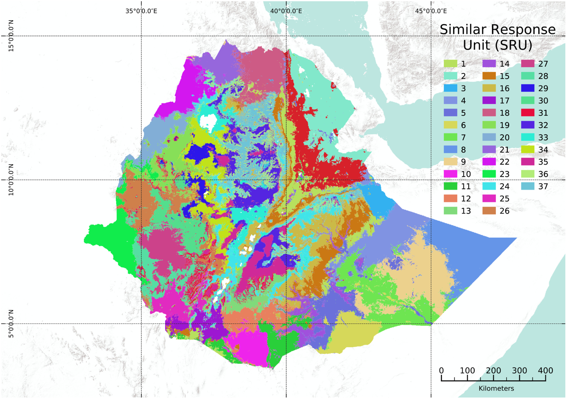
Figure 6. The pattern and spatial distribution of optimal SRUs based on X-means clustering algorithm.
In principle, each SRU can be attributed using various environmental variables and users can obtain SRU properties for further scrutiny. However, owing to the heterogeneity of Ethiopia’s landscape, specifically the highlands, the role of different attributes in creating the SRUs is complex (Figure 6). In order to facilitate interpretation, spatially aggregated mean value for all the covariates at SRU level (associated with Figure 6) is provided in Appendix I (Table A1). Users can compile the legend following the major environmental characteristics of each unit using the table provided with the statistics of each covariate in the clusters (Appendix I, Table A1).
Performance of the clustering and validity of SRU maps
The outputs shown in Figures 5 and 6 were presented to national experts who have come from different parts of the country and are familiar with the farming systems. The idea was to discuss the ‘concept of SRUs’ and assess the results. The participants appreciated the need to develop an automated system that can enable deriving clusters that can be used for targeting interventions. They also stressed the generality of the existing AEZs to repressing the heterogeneity of the farming systems and challenge to ascribe targeted advisories. After checking the various clusters, it was agreed that SRU with 9 clusters is too general while SRU with 53 clusters is too detailed and complex to comprehend visually. Considering this, the participants indicated the relevance and applicability of clusters 30 and 37 to facilitate agricultural decision making. These maps have captured heterogeneity well, while at the same time the number of clusters is optimal to manage for operational purposes. This, among others, is because the refined zonation can be used to provide detailed and location-specific advisories that will not be possible at generalised levels. The intermediate level of classification can also overcome the difficulty to develop and prescribe advisories at plot level (too detailed). However, the experts suggested the need to validate the results properly using quantitate and field data.
The other assessment was based on comparing the distribution of standard deviation of optimal crop response to fertiliser application between the existing AEZ and the SRUs with the same number of clusters (Figure 7). The result shows that for the same level of 7 and 15 clusters, the approach used in this study produced a lower standard deviation value than the AEZs for all of Ethiopia. This suggests that the use of SRUs for targeting fertiliser recommendation is preferable as it contains more homogeneous units in terms of response to fertiliser application; however, this changes when the number of clusters increases. The standard deviation of response to fertiliser application becomes similar when we compare AEZ and SRU clusters of 33 units. This basically suggests the advantage of a larger number of clusters that can capture heterogeneity better for agricultural technology targeting and recommendation. This was also corroborated by the experts’ opinions. Future analysis will use field data related to integrated soil fertility management to assess the optimal number of clusters that can capture variability across space and scale.
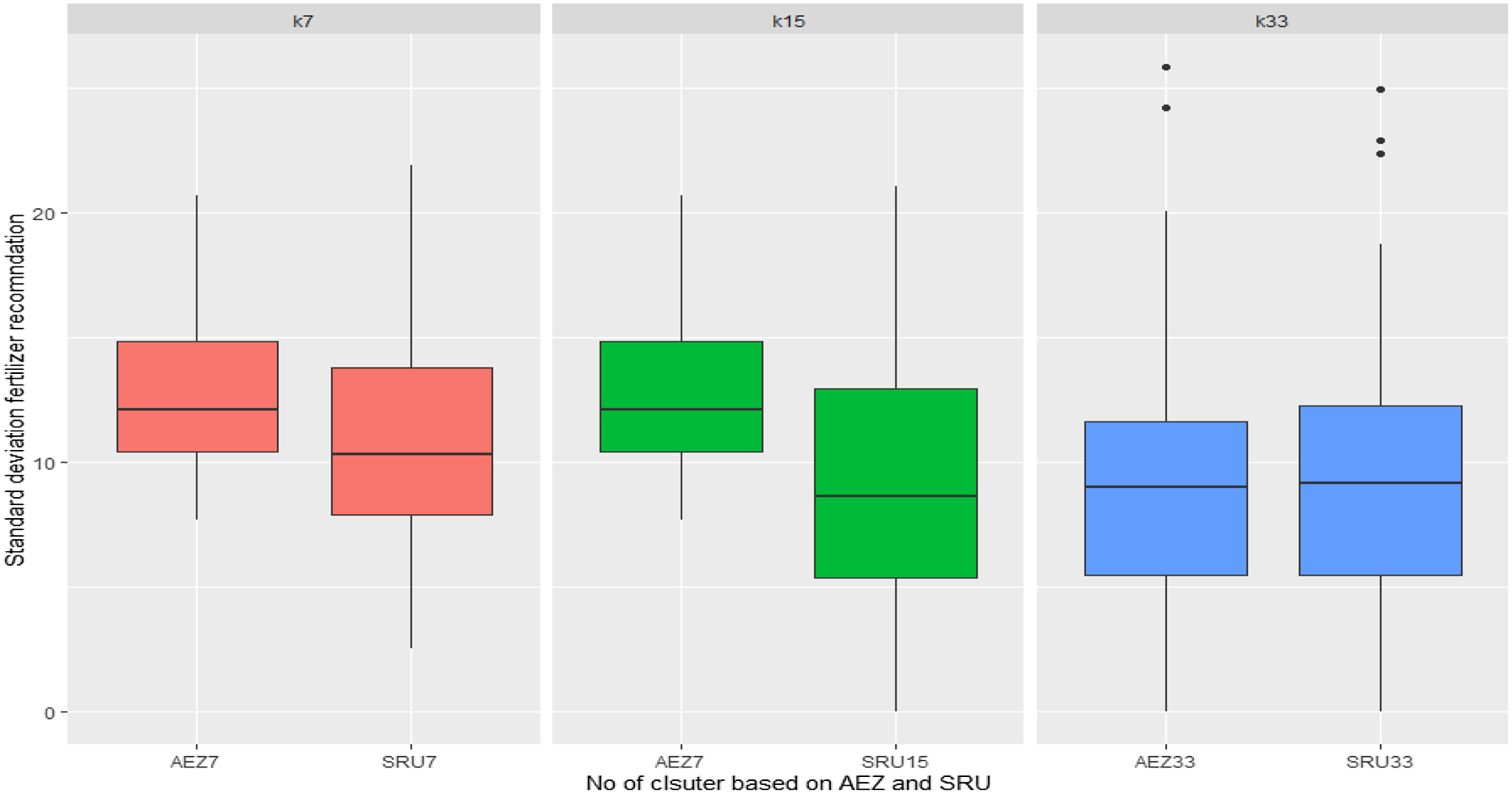
Figure 7. Standard deviation of recommended nitrogen fertiliser according to the agro-ecological zones and classification approach used in this study.
Generally, it is noted that the ‘classification approach’ is essential for planning and targeting in situations where broader agro-ecological and farming system approaches are not plausible and, at the same time, plot-level interventions/advisories cannot be developed at the current state of data availability, especially in developing countries.
Clustering tool and reproducibility
Over the past few decades, widespread availability of spatial data and the advancement of robust modelling algorithms have increased. Such developments are creating unique opportunities that help answer targeted questions and prioritisations related to optimisation of natural resource management as well as steps to be taken for economic development and facilitation of poverty alleviation on the basis of recommendation domains (Akıncı et al., Reference Akıncı, Özalp and Turgut2013; Elsheikh et al., Reference Elsheikh, Shariff, Amiri, Ahmad, Balasundram and Soom2013; Hyman et al., Reference Hyman, Hodson and Jones2013). Jasiewicz et al. (Reference Jasiewicz, Netzel and Stepinski2014) introduced landscape similarity mapping using a numerical measure that assesses affinity between different landscapes based on the similarity between the patterns of their constituent landform elements. Automating the operationalisation of such techniques using similar and standard data sets can enable standardisation of the approaches and comparison of associated results. A study by Muthoni et al. (Reference Muthoni, Guo, Bekunda, Sseguya, Kizito, Baijukya and Hoeschle-Zeledon2017) used geospatial analysis and clustering techniques to delineate relatively similar clusters for scaling improved crop varieties and good agronomic practices. This approach added value to the previous ones by providing options to compare different clustering approaches.
In this study, we moved one step further in order to allow users access to relevant data from the cloud and/or add their own data and choose a specific geographical area of interest to run clustering. We developed a generic framework that supports creating a scalable system to be used to delineate SRUs for different purposes. The data analytics component provides options for several clustering methods (e.g. partitioning, distribution-based, hierarchical and fuzzy). The classification algorithm is also designed such that it can be scalable to run analysis for different extents but maintaining a standard procedure. The functionality of the system thus enables accessing data from the cloud, running clustering for a defined geographical area of interest and automatically performing clustering for different agronomic purposes.
The whole process is automated in an R programming environment and piloted for Ethiopia using globally available geospatial data. The system being put in place is generic and is being expanded to create a clustering analytic platform. The platform gives reproducible results which allow users to interactively choose data sources, use expert knowledge, experiment and compare the result of several algorithms and be flexible in order to work at any spatial scale and resolution to provide SRUs for interventions for sub-Saharan African countries. The tool generated is available for the public in an open repository (https://github.com/EiA2030/validation), including the workflows generated in this study.
Conclusion and Future Research Direction
Matching agricultural operations and inputs to the crop requirement, as is the case with precision agriculture, requires understanding the within-field variation of underlying biophysical factors. Because real-time monitoring and tailoring farm management to field-level variation are not possible, an alternative option is classifying the target area into homogenous units. This exercise becomes increasingly important to enhance agricultural productivity under optimised resource use for areas with fragmented farming systems and heterogeneous landscapes, as is the case in Ethiopia. To benefit from such advances, the current effort is made to create a scalable and operational tool that can harvest relevant data from the cloud and enable users to partition areas into uniform zones. The tool and its generic workflow have been piloted for Ethiopia.
The workflow and automated system demonstrated in this study can be used to create homogeneous landscape units using different clustering algorithms. The system is flexible to allow users to either refine or run targeted zoning as more relevant data are made available. The study serves to demonstrate the possibility of aggregating SRUs in a standardised way, ensuring transferability to other regions and settings. Although the algorithms used in this study are standard packages available in commonly used statistical software, the power of the system presented here is the practical convenience of offering an integrated solution whereby users could readily source the relevant data for different geographies, run the data analytics and obtain reproducible results including submission of the study area with defined territory.
The approach in this study targeted the use of global coverage data (or available at the scale of interest) that can be harvested from the cloud and harmonised for integrated analysis. As a result, some important data/variables that are not commonly available or that have questionable accuracy have not been used. For instance, geomorphology is an important factor that relates soil types with topographic catena and is among the major components of soil-forming factors. However, geomorphology data were not used in this study because we doubted the quality of the existing data a national scale. Such addititional data and improved analityics can improve the results.
The approach employed in this study demonstrates its potential to zoning spatial geographies into uniform clusters. Next steps will focus on validation the SRUs using ‘ground information’ and fine-tune their applicability. In addition, an attempt will be made to develop SRUs that will be specific to target defined issues such as climate-smart agriculture and other agronomic practices. In addition, functionalities will be incorporated to provide more options to the user (e.g. masking out non-agricultural areas) and assessing performances in an automated manner.
Acknowledgements
We thank the Supporting Soil Health Initiatives (SSHI) of GIZ-Ethiopia project for its support to gather data and conduct analysis. The Excellence in Agronomy (EiA) team provided great input and advnaced the analytics. The Africa RISING project funded by United States Agency for International Development and Feed the Future; and the Accelerating Impacts of CGIAR Climate Research in Africa (AICCRA) projects have also supported staff time of some of the authors. In addition, we recognise the support from the Water, Land and Ecosystems programme of the CGIAR as well as the European Union–International Fund for Agricultural Development project under the CGIAR Research Program on Climate Change, Agriculture and Food Security. We are also indebted to the great support of the ‘coalition of the willing’ members who were instrumental in generating various ideas and supporting analytics including providing data sets.
Funding Support
This work was supported, in whole or in part, by the Bill & Melinda Gates Foundation [INV-005460]. Under the grant conditions of the Foundation, a Creative Commons Attribution 4.0 Generic License has already been assigned to the Author Accepted Manuscript version that might arise from this submission.
Data Availability Statement
The data used to produce this article is available and accessible.
Conflict of Interest
We declare that there is no conflict of interest associated with all co-authors.
Appendix A
Table A1. The mean value for each environmental attribute associated with each cluster mapped in Figure 6
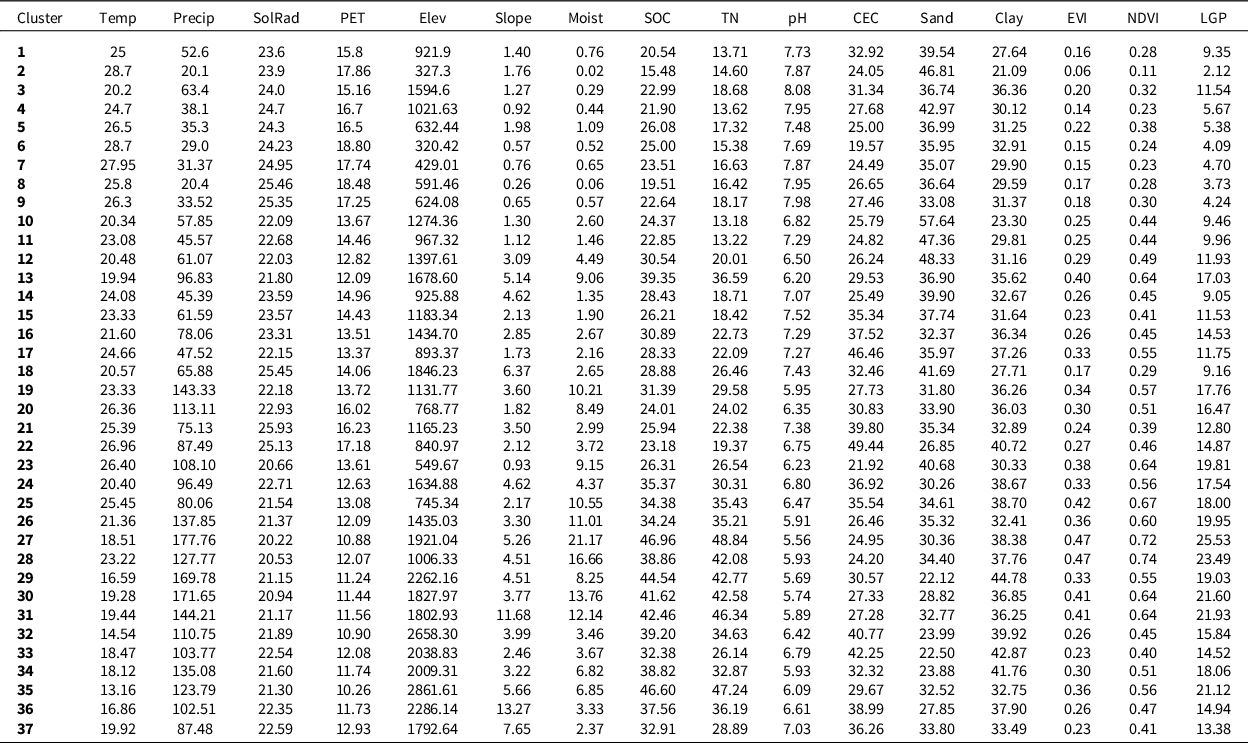
Temp: annual mean temperature; Precip: annual mean precipitation in mm; SolRad: net solar radiation in W/m2; PET: potential evapotranspiration in mm; elev: elevation in metre; slope: slope in %; moist: soil moisture in mm; SOC: soil organic carbon in g/kg; TN: total nitrogen in g/kg; pH: soil pH; cation exchange capacity in cmol/kg; sand: sand in %; clay: clay in %; EVI: enhanced vegetation index; NDVI: net difference vegetation index; LGP: length of the growing period.


 Open access