


1 Introduction
In view of the changing energy demands and supplies, the combined and intertwined energy networks are expected to play a prominent role in the future. Here, the additional but unpredictable and volatile energy sources need to be complemented with traditional means of production as well as possibly additional large-scale storage [51, Reference Zablocki54]. Following previous approaches [Reference Chertkov, Backhaus and Lebedev17, Reference Zeng55, Reference Zlotnik57], we consider here energy storage through coupling power networks to gas networks. The latter are able to generate sufficient power at times when renewable energy might not be available or vice versa convert energy to ramp up pressure in the gas networks, see for example [Reference Brown14, Reference Heinen, Burke and O’Malley31, Reference Schiebahn48]. A major concern when coupling gas and power networks is guaranteeing a stable operation even at times of stress due to (uncertain) heavy loads. The propagation of possible uncertain loads on the power network and its effect on the gas network has been subject to recent investigation, and we refer to [Reference Chertkov, Backhaus and Lebedev17] and references therein. Contrary to the cited reference [Reference Chertkov, Backhaus and Lebedev17], we are interested here in a full simulation of both the gas and the power network as well as the simulation of the stochastic demand and, respectively, supply. This will allow for a prediction at all nodes as well as study dynamic effects changing supplies and demands in the network.
Regarding the underlying models for simulation, we rely on established power flow (PF), gas flow and stochastic demand models that will be briefly reviewed in the following. PF is typically modelled through prescribing real and reactive power at nodes of the electric grid. Their values are obtained through a nonlinear system of algebraic equations. Supply and demand can be time–dependent requiring to frequently resolve the nonlinear system. For more details on the model, we refer to [Reference Bienstock, Chertkov and Harnett10, Reference Capitanescu15, Reference Faulwasser21, Reference Frank and Rebennack25, Reference Low38, Reference Low39, Reference Mühlpfordt and Syst42] as well as to the forthcoming section where the equations are reviewed. While propagation of electricity is typically assumed to be instantaneous as in the PF equations, the propagation of gas in networks has an intrinsic spatial and temporal scale. A variety of models exist nowadays, and we follow here an approach based on hyperbolic balance laws as proposed for example in [Reference Banda, Herty and Klar5, Reference Banda, Herty and Klar6, 11, Reference Brouwer, Gasser and Herty12, Reference Colombo and Garavello19]. This description allows the prediction of gas pressure and gas flux at each point in the pipe as well as nodes of the network. Both quantities are relevant to assess possible stability issues as well as allow for coupling towards the electricity network. The numerical solution of the governing gas equations as well as their coupling towards electricity and towards other gas pipelines is also detailed in the forthcoming section. Finally, we recall recent results on modelling of the prediction of the electricity demand that will be used to simulate the uncertain power fluctuations. Here, we follow models introduced in [Reference Aïd1, Reference Barlow7, Reference Kiesel, Schindlmayr and Börger34, Reference Lucia and Schwartz40, Reference Schwartz and Smith47, Reference Wagner53] and the monograph [Reference Benth, Benth and Koekebakker8] that prescribe the electricity demand as Ornstein–Uhlenbeck processes (OUP). Let us emphasise that our approach is not limited to the particular application of gas transportation but could eventually be applied to problems of traffic flow and supply chain dynamics on networks.
Finally, we point to other existing numerical simulations with possibly similar objective. For example, in [Reference Kolb36] a solver for a gas network based on (general) hyperbolic balance laws has been introduced. This implementation serves as foundation for the method introduced in the forthcoming section. Our tool has the advantage of easier extensibility, an open source license and a modern design approach featuring, for example, extensive software testing. In addition, we also include stochastic power demands in the PF network setting. In [Reference Anderson, Turner and Koch4], uncertainty in PF is computed relying on approaches based on neural networks. A difference to the presented approach is the restriction to linear PF problems and the absence of coupling to gas networks. A further concept plan4res, see [Reference Beulertz9] has been presented to also address general renewable energy sources as well as energy distribution based on discrete optimisation approaches, which focuses on energy system modelling in more generality. Furthermore, there exists a software suite by Fraunhofer SCAI called MYNTS, see [Reference Clees18], that also includes simulation and optimisation of inter-connected grid operations with a focus on the design of suitable networks. The paper is organised as follows: In Section 2, we introduce the model equations for the coupled network setting and the uncertain demand. The numerical discretisation is then given in Section 3. Section 4 is concerned with the presentation of our software suite and the numerical investigation of relevant scenarios.
2 Mathematical modelling
In this section, we introduce the mathematical models to be discretised in the forthcoming section. We denote by $\mathcal{G}=(\mathcal{N},\mathcal{A})$
a directed graph with a set of nodes
$\mathcal{G}=(\mathcal{N},\mathcal{A})$
a directed graph with a set of nodes $\mathcal{N}$
and a set of arcs
$\mathcal{N}$
and a set of arcs $\mathcal{A}$
. All dynamics are either on nodes and/or on arcs of the graph. The whole graph is sub-divided into a power network, a gas network and a set of arcs connecting these two:
$\mathcal{A}$
. All dynamics are either on nodes and/or on arcs of the graph. The whole graph is sub-divided into a power network, a gas network and a set of arcs connecting these two:
 \begin{align*} \mathcal{G} &= \mathcal{G}_{\text{P}} \cup\mathcal{G}_{\text{G}} \cup\mathcal{G}_{\text{GP}}\\[3pt] \mathcal{N} &= \mathcal{N}_{\text{P}} \cup\mathcal{N}_{\text{G}} \cup\mathcal{N}_{\text{GP}}\\[3pt] \mathcal{A} &= \mathcal{A}_{\text{P}} \cup\mathcal{A}_{\text{G}} \cup\mathcal{A}_{\text{GP}}. \end{align*}
The different parts behave quite differently. In the power network, the arcs just carry two parameters and their topological information, that is their starting and ending node and the nodes carry most of the physical information, namely active and reactive power, while the situation in the gas network is reversed. Here the arcs carry a balance law describing gas dynamics while the nodes only carry coupling information. Yet in all parts of the network, only the nodes have (possibly stochastic) boundary conditions.Footnote 1 The gas power connection part of the network consists only of arcs which relate power demand and gas consumption or gas generation and power surplus. An illustration of such a network can be found in Figure 1.

Figure 1. A schematic example of the kind of network under consideration. The upper right part is a power network with blue slack nodes, green power plants and red load nodes. In the lower left, there is a gas network with pipelines between junctions. The doubly pointed arc is a gas power connection.
Next, we define model equations for each node and arc (where applicable) based on physical models.
2.1 PF equations modelling electric PF on $\mathcal{G}_\boldsymbol{P}$

The evolution of reactive and active power at nodes is modelled by the PF equations [Reference Grainger, Stevenson and Chang28]. This model can be used to describe the behaviour of power networks operating at sinusoidal alternating current (AC) [Reference Fokken and Göttlich22]. The quantities modelled are the active or real power $P_k=P_k(t)$
and the reactive power
$P_k=P_k(t)$
and the reactive power $Q_k=Q_k(t)$
present at each node
$Q_k=Q_k(t)$
present at each node $k\in\mathcal{N}_{\text{P}}$
at time t. Those are functions of the voltage magnitude
$k\in\mathcal{N}_{\text{P}}$
at time t. Those are functions of the voltage magnitude $V_k$
and angle
$V_k$
and angle $\phi_k$
. Further, we model the admittance of each component, denoted by Y, which is written into real and imaginary part
$\phi_k$
. Further, we model the admittance of each component, denoted by Y, which is written into real and imaginary part $Y = G+\text{i} B$
. The admittance is the inverse of the impedance which in turn is a complex extension of Ohmic resistance in the power network.
$Y = G+\text{i} B$
. The admittance is the inverse of the impedance which in turn is a complex extension of Ohmic resistance in the power network.
The admittance of a transmission line, that is, an arc $a \in \mathcal{A}_{\text{P}}$
connecting nodes
$a \in \mathcal{A}_{\text{P}}$
connecting nodes $i,k \in \mathcal{N}_P,$
is denoted by
$i,k \in \mathcal{N}_P,$
is denoted by $Y_{ik} = G_{ik}+\text{i} B_{ik}$
, which we set to zero, if no arc connects i and k. The admittance of a node
$Y_{ik} = G_{ik}+\text{i} B_{ik}$
, which we set to zero, if no arc connects i and k. The admittance of a node $k \in \mathcal{N}_P$
is denoted by
$k \in \mathcal{N}_P$
is denoted by $Y_{kk} = G_{kk}+\text{i} B_{kk}$
.
$Y_{kk} = G_{kk}+\text{i} B_{kk}$
.
With this, we can write down the PF equations, a set of $2 | \mathcal{N}_P | $
equations at any point t in time of the type
$2 | \mathcal{N}_P | $
equations at any point t in time of the type
 \begin{equation} \begin{aligned} P_{k}(t) & = \sum_{i \in \mathcal{N}_{\text{P}}} V_k(t)V_i(t)(G_{ki}\cos(\phi_k(t)-\phi_i(t))+B_{ki}\sin(\phi_k(t)-\phi_i(t))),\\[3pt] Q_{k}(t) & = \sum_{i \in \mathcal{N}_{\text{P}}} V_k(t)V_i(t)(G_{ki}\sin(\phi_k(t)-\phi_i(t))-B_{ki}\cos(\phi_k(t)-\phi_i(t))), \end{aligned}\end{equation}
for the unknowns $(P_k(t),Q_k(t),V_k(t),\phi_k(t)) k \in \mathcal{N}_P$
. In order to obtain a unique solution, additional
$(P_k(t),Q_k(t),V_k(t),\phi_k(t)) k \in \mathcal{N}_P$
. In order to obtain a unique solution, additional $2| \mathcal{N}_P |$
equality constraints have to be specified. We distinguish three different equality constraints according to the type of node
$2| \mathcal{N}_P |$
equality constraints have to be specified. We distinguish three different equality constraints according to the type of node $k\in \mathcal{N}_P$
:
$k\in \mathcal{N}_P$
:
-
Slack nodes k specify values for the voltage magnitudes and angles
$V_k,\phi_k$
. -
Load nodes k specify values for the active and reactive power
$P_k,Q_k$
. -
Generators k specify values for the active power and voltage magnitude
$P_k,V_k$
.


A necessary condition for uniqueness of the PF equations is to have at least one slack node, because otherwise for a solution $(P_k(t),Q_k(t),V_k(t),\phi_k(t)) k \in \mathcal{N}_P$
with
$(P_k(t),Q_k(t),V_k(t),\phi_k(t)) k \in \mathcal{N}_P$
with $r \in \mathbb{R}$
, a second solution is given by
$r \in \mathbb{R}$
, a second solution is given by $(P_k(t),Q_k(t),V_k(t),\phi_k(t)+r) k \in \mathcal{N}_P$
. Often only a single slack node is used, although also multiple slack nodes can be used [Reference Chayakulkheeree16].
$(P_k(t),Q_k(t),V_k(t),\phi_k(t)+r) k \in \mathcal{N}_P$
. Often only a single slack node is used, although also multiple slack nodes can be used [Reference Chayakulkheeree16].
Instead of the described AC PF equations, it is possible to use so-called direct current (DC) PF equations, which are a linear approximation, see [Reference Glover and Sarma27, 6.10] for an overview. This approach simplifies the numerical treatment greatly at the cost of some accuracy. Other linearisations are subject of active research, see for example [Reference Li, Pan and Liu37].
2.2 Mathematical modelling of gas flow on
$\mathcal{G}_{\text{G}}$

We model the following quantities of the gas flow, namely the pressure $p=p(t,x)$
as well as the flux
$p=p(t,x)$
as well as the flux $q=q(t,x)$
. The units of those quantities are (bar) and
$q=q(t,x)$
. The units of those quantities are (bar) and $\mathrm{m}^{3}\ \mathrm{s}^-1$
. Note that we use the volumetric flow as opposed to mass flow, as is customary in real-world gas networks. The pressure is given by a function of the gas density
$\mathrm{m}^{3}\ \mathrm{s}^-1$
. Note that we use the volumetric flow as opposed to mass flow, as is customary in real-world gas networks. The pressure is given by a function of the gas density $\rho=\rho(t,x)$
. An overview as well as recent results on gas flow can be found for example in [Reference Banda, Herty and Klar5, Reference Banda, Herty and Klar6, 11, Reference Brouwer, Gasser and Herty12, Reference Colombo and Garavello19, Reference Reigstad44, Reference Reigstad45]
$\rho=\rho(t,x)$
. An overview as well as recent results on gas flow can be found for example in [Reference Banda, Herty and Klar5, Reference Banda, Herty and Klar6, 11, Reference Brouwer, Gasser and Herty12, Reference Colombo and Garavello19, Reference Reigstad44, Reference Reigstad45]
2.2.1 Transport of gas along pipelines
The direction of the arcs determines the positive direction of the flow. We distinguish two types of arcs, pipelines and controlled arcs, which are described in the next Section 2.2.2. In contrast to the power arcs, pipelines $a \in \mathcal{A}_{\text{G}}$
in the gas network are modelled as an interval
$a \in \mathcal{A}_{\text{G}}$
in the gas network are modelled as an interval $[0,L_a]$
with further structure. The gas flow in pipelines is modelled with the isentropic Euler equations as for example proposed in [Reference Banda, Herty and Klar5].
$[0,L_a]$
with further structure. The gas flow in pipelines is modelled with the isentropic Euler equations as for example proposed in [Reference Banda, Herty and Klar5].
The conservative variables are the gas density $\rho$
and the flux q. Consider an arc
$\rho$
and the flux q. Consider an arc $a \in \mathcal{A}_{\text{G}}$
parametrised by
$a \in \mathcal{A}_{\text{G}}$
parametrised by $x \in (0,L_a)$
. Then, the density
$x \in (0,L_a)$
. Then, the density $\rho=\rho_a(t,x)$
and
$\rho=\rho_a(t,x)$
and $q=q_a(t,x)$
fulfil in the weak sense the following system of hyperbolic balance laws for each
$q=q_a(t,x)$
fulfil in the weak sense the following system of hyperbolic balance laws for each $t\geq 0$
.
$t\geq 0$
.
 \begin{equation} \begin{pmatrix}\rho\\ \\[-7pt] q\end{pmatrix}_t + \begin{pmatrix} \frac{\rho_0}{A}q\\ \\[-7pt] \frac{A}{\rho_0}p(\rho) + \frac{\rho_0}{A}\frac{ q^2}{\rho}\end{pmatrix}_x = \begin{pmatrix}0\\ \\[-7pt] S(\rho, q) \end{pmatrix}.\end{equation}
Here S is the source term modelling wall friction in the pipes detailed below, A is the cross-section of the pipe, $\rho_0$
is the (constant) density of the gas under standard conditions, and p is the pressure function, which we describe in detail below. First we note that the system (2.2) is accompanied by initial conditions
$\rho_0$
is the (constant) density of the gas under standard conditions, and p is the pressure function, which we describe in detail below. First we note that the system (2.2) is accompanied by initial conditions
 \begin{align} \rho(0,x)=\rho_{0,a}(x), \; q(0,x)=q_{0,a}(x)\end{align}
that may also dependent on the selected arc a and describe the initial state of density and flux. Suitable boundary conditions at $x=0$
and
$x=0$
and $x=L_a$
will be discussed below when the coupling at nodes of the network is introduced.
$x=L_a$
will be discussed below when the coupling at nodes of the network is introduced.
The pressure p is a function of the density given by
 \begin{equation} p(\rho) = \frac{c_{\text{vac}}^2\rho}{1-\alpha c_{\text{vac}}^2 \rho},\end{equation}
where $c_{\text{vac}}$
is the vacuum limit (
$c_{\text{vac}}$
is the vacuum limit ( $\rho \to 0$
) of the speed of sound and
$\rho \to 0$
) of the speed of sound and $\alpha$
is a measure of compressibility of the gas. The relevant constants of the gas network are gathered in Table 1. It is possible to express the density in terms of the pressure as
$\alpha$
is a measure of compressibility of the gas. The relevant constants of the gas network are gathered in Table 1. It is possible to express the density in terms of the pressure as
 \begin{equation} \rho = \frac{p}{c_{\text{vac}}^2 z(p)},\end{equation}
where $z(p) = 1+\alpha p$
is the so-called compressibility factor.
$z(p) = 1+\alpha p$
is the so-called compressibility factor.
Table 1. Gas net constants

The source term S is given as
 \begin{equation} S(\rho,q) = \frac{\lambda(q)}{2d} \frac{\lvert q \rvert}{\rho} \left( -q \right),\end{equation}
where now d is the pipe diameter and $\lambda(q)$
is the flux-dependent Darcy friction factor, see [Reference Brown13]. The friction is governed by the so-called Reynolds number,
$\lambda(q)$
is the flux-dependent Darcy friction factor, see [Reference Brown13]. The friction is governed by the so-called Reynolds number,
 \begin{equation} \mathrm{Re}(q) = \frac{d}{A\eta}\rho_0\lvert q \rvert\end{equation}
(here $\eta = 10^{-5} \mathrm{kg\ m}^{-1} \mathrm{s}^{-1}$
is the dynamic viscosity of the gas). For
$\eta = 10^{-5} \mathrm{kg\ m}^{-1} \mathrm{s}^{-1}$
is the dynamic viscosity of the gas). For $\mathrm{Re} <2000, $
the friction is dominated by laminar flow, and according to [Reference Menon41], we may assume
$\mathrm{Re} <2000, $
the friction is dominated by laminar flow, and according to [Reference Menon41], we may assume
 \begin{equation} \lambda(q) = \frac{64}{\mathrm{Re}(q)}.\end{equation}
For $\mathrm{Re} > 4000, $
the friction is dominated by turbulent flow, see again [Reference Menon41], and the Swamee-Jain approximation [Reference Swamee and Jain50] is used, that is,
$\mathrm{Re} > 4000, $
the friction is dominated by turbulent flow, see again [Reference Menon41], and the Swamee-Jain approximation [Reference Swamee and Jain50] is used, that is,
 \begin{equation} \lambda(q) = \frac{1}{4} \frac{1}{\mathrm{ld}(\frac{k}{3.7 d} + \frac{5.74}{\mathrm{Re}^{0.9}})^2}.\end{equation}
For Re in the intermediate regime, the numbers are interpolated using a cubic polynomial differentiable at $\mathrm{Re} \in \{ 2000, 4000 \}$
.
$\mathrm{Re} \in \{ 2000, 4000 \}$
.
2.2.2 Controlled gas arcs
In addition to pipes, the considered gas network also contains a compressor and a control valve. Both are modelled similarly and come equipped with a control function u that influences the pressure.
Both valves and compressors do not influence the flow rate of the gas inside them, so at every time point t there must hold
 \begin{equation} q_{\text{out}}(t) = q_{\text{in}}(t).\end{equation}
Yet for the pressure, we set in compressors
 \begin{equation} p_{\text{out}}(t) = p_{\text{in}}(t)+u(t),\end{equation}
and in valves
 \begin{equation} p_{\text{out}}(t) = p_{\text{in}}(t)-u(t),\end{equation}
such that the control can change the pressure. For other possible compressor models, see for example [Reference Kolb36]. In addition, we demand $u(t)\geq 0$
for both component types. Also for the purpose of optimisation, using the compressor comes with a cost, while using the valve is free. Note that for the main part of this work, both valves and compressors are in-active meaning a control function of
$u(t)\geq 0$
for both component types. Also for the purpose of optimisation, using the compressor comes with a cost, while using the valve is free. Note that for the main part of this work, both valves and compressors are in-active meaning a control function of $u(t)=0$
. Only in the optimisation example, a non-zero control is allowed.
$u(t)=0$
. Only in the optimisation example, a non-zero control is allowed.
2.2.3 Nodes of the gas network
$\mathcal{N}_G$

The previous set of differential equations has to be accompanied by boundary conditions if $L_a<\infty.$
For nodes
$L_a<\infty.$
For nodes $n \in \mathcal{N}_G$
the coupling of gas pipelines is typically described in terms of coupling conditions [Reference Herty32]. Those yield an implicit description of the boundary values in terms of physical relations. Several different conditions exist, see [Reference Holle, Herty and Westdickenberg33, Reference Reigstad44, Reference Reigstad45]. Yet, for the purpose of real-world gas pipelines, [Reference Fokken, Herty and Milde24] seems to indicate that coupling via equality of pressure is sufficient for the expectable accuracy of the whole modelling approach. Therefore, consider a node
$n \in \mathcal{N}_G$
the coupling of gas pipelines is typically described in terms of coupling conditions [Reference Herty32]. Those yield an implicit description of the boundary values in terms of physical relations. Several different conditions exist, see [Reference Holle, Herty and Westdickenberg33, Reference Reigstad44, Reference Reigstad45]. Yet, for the purpose of real-world gas pipelines, [Reference Fokken, Herty and Milde24] seems to indicate that coupling via equality of pressure is sufficient for the expectable accuracy of the whole modelling approach. Therefore, consider a node $n \in \mathcal{N}_G $
with K adjacent arcs. Let
$n \in \mathcal{N}_G $
with K adjacent arcs. Let $E \subset \mathcal{A}$
denote the set of adjacent arcs and let
$E \subset \mathcal{A}$
denote the set of adjacent arcs and let
 \begin{align} &s: E \to \{\pm 1\}, \nonumber\\[3pt] &s(e) = \begin{cases} \phantom{-{}}1\ &e \text{ starts in } n\\ -1\ &e \text{ ends in } n\\ \end{cases} \end{align}
distinguish arcs starting and ending in n. Also, let $p_e(t),q_e(t)\ e \in E$
denote the boundary values at time t of arc e in node n, that is,
$p_e(t),q_e(t)\ e \in E$
denote the boundary values at time t of arc e in node n, that is, $p_e = p_e(t,x=0)$
if
$p_e = p_e(t,x=0)$
if $s(e)=1$
and
$s(e)=1$
and $p_e(t)=p_e(L_a,t)$
if
$p_e(t)=p_e(L_a,t)$
if $s(e)=-1$
and similarly for
$s(e)=-1$
and similarly for $q_e.$
Then, the coupling and boundary conditions at node n read
$q_e.$
Then, the coupling and boundary conditions at node n read
 \begin{equation} \begin{aligned} p_e(t) &= p_f(t) \text{ for all } e,f \in E \\ \\[-7pt] q_n(t) &= \sum_{e \in E}s(e)q_e(t), \end{aligned}\end{equation}
where $q_n:\mathbb{R}^+_0 \to \mathbb{R}$
a possibly time-dependent external and given demand or supply function. These are in total
$q_n:\mathbb{R}^+_0 \to \mathbb{R}$
a possibly time-dependent external and given demand or supply function. These are in total $\lvert E \rvert$
equations at node n at each point in time.
$\lvert E \rvert$
equations at node n at each point in time.
For a single node with K adjacent arcs extending to infinity and under subsonic condition for the initial data existence of weak entropic solutions in BV has been shown for example in [Reference Colombo and Garavello19]. In [Reference Holle, Herty and Westdickenberg33], existence of weak integrable solutions on a graph has been established. Similar results are also available for other choices of coupling conditions, and we refer to for example [Reference Brouwer, Gasser and Herty12].
2.3 Modelling of Gas-to-Power or Power-to-Gas nodes
$\mathcal{N}_{\text{GP}}$

Gas power plants are also modelled as arcs in the graph connecting a power node and a gas node. They transform gas into power at a linear rate and also power into gas at a (different) linear rate as was done in [Reference Fokken, Herty and Milde24]. At the switching point, we smooth the resulting kink with a polynomial. This has no physical counterpart and is done purely for numerical reasons. Note that due to technical reasons, our polynomial maps gas flow to power instead of the other way around as was chosen in [Reference Fokken, Herty and Milde24]. For the power output of the gas power plant, there holds
 \begin{equation} P = \begin{cases} E_{\text{PtG}}\cdot q &\text{ for } \phantom{ {}- \kappa < {}} q<-\kappa\\ \\[-7pt] \text{pol}(q) &\text{ for } -\kappa <q<\kappa \\\\[-7pt] E_{\text{GtP}}\cdot q &\text{ for } \phantom{{}-{}}\kappa<q \end{cases}\ ,\end{equation}
where $E_{\text{PtG}}$
and
$E_{\text{PtG}}$
and $E_{\text{GtP}}$
are the efficiencies of the power-to-gas process and the gas burning respectively, and pol is the interpolating polynomial. For
$E_{\text{GtP}}$
are the efficiencies of the power-to-gas process and the gas burning respectively, and pol is the interpolating polynomial. For $\kappa,$
we choose
$\kappa,$
we choose $\kappa = 60 \mathrm{m}^{3} \mathrm{s}^{-1}$
. The power is taken as the real power of the attached power node, which is a slack node and therefore provides via the solution of the PF problem a real power demand.
$\kappa = 60 \mathrm{m}^{3} \mathrm{s}^{-1}$
. The power is taken as the real power of the attached power node, which is a slack node and therefore provides via the solution of the PF problem a real power demand.
2.4 Stochastic power nodes
$\mathcal{N}_{\text{P}}$

In order to incorporate uncertain power demands into our model, we add a new kind of load node, the stochastic PQ-node. The type of uncertainty employed, the OUP, has a long history in modelling uncertain demands of various types and has also been used for electricity demand, see [Reference Barlow7, Reference Göttlich, Kolb and Lux26]. In [Reference Göttlich, Kolb and Lux26], a setting similar to ours was examined but applied to the Telegrapher’s equations instead of the PF equations.
The stochastic PQ-node, just like its deterministic cousin, prescribes a real and reactive power demand as boundary conditions but now these demands are stochastic time-dependent quantities modelling the uncertainty of demand at this node. Of course, this uncertainty is not total, as one may expect the demand to follow historic timelines of demand or some other estimate derived from knowledge about the season, weather or even current events like a sports tournament. This structure of uncertain fluctuation about a deterministic estimate suggests using a mean reverting stochastic process for the power demand, $\left(P_t\right)_{t \in [0,T]}$
, that is, a process that is drawn back to some deterministic function
$\left(P_t\right)_{t \in [0,T]}$
, that is, a process that is drawn back to some deterministic function $\mu(t)$
over time. If we further assume that fluctuations around
$\mu(t)$
over time. If we further assume that fluctuations around $\mu$
are independent of the current time and also of the current value of P, a natural choice for the process is the OUP. It is characterised by the following stochastic differential equation,
$\mu$
are independent of the current time and also of the current value of P, a natural choice for the process is the OUP. It is characterised by the following stochastic differential equation,
 \begin{align} dP_t=\theta\left(\mu(t)-P_t\right)dt + \sigma dW_t,\ \quad P_{t_0}=p_{0},\end{align}
where $W_t$
is a one-dimensional Brownian motion,
$W_t$
is a one-dimensional Brownian motion, $\theta,\sigma >0$
are the so-called drift and diffusion coefficients, and
$\theta,\sigma >0$
are the so-called drift and diffusion coefficients, and $p_{0}$
is the demand at the starting time
$p_{0}$
is the demand at the starting time $t_0$
.
$t_0$
.
Whenever the current demand $P_t$
differs from
$P_t$
differs from $\mu(t)$
, the drift term enacts a force towards the deterministic demand estimate
$\mu(t)$
, the drift term enacts a force towards the deterministic demand estimate $\mu(t)$
. This behaviour is called mean reversion. The size of this force is characterised by the drift coefficient
$\mu(t)$
. This behaviour is called mean reversion. The size of this force is characterised by the drift coefficient $\theta$
. In absence of diffusion (for
$\theta$
. In absence of diffusion (for $\sigma = 0$
), the OUP degenerates to a deterministic ordinary differential equation, that is drawn to the mean exponentially. For
$\sigma = 0$
), the OUP degenerates to a deterministic ordinary differential equation, that is drawn to the mean exponentially. For $\sigma >0$
on the other hand, this mean reversion is counteracted by fluctuations, whose size is determined by
$\sigma >0$
on the other hand, this mean reversion is counteracted by fluctuations, whose size is determined by $\sigma$
. For images of OUP realisations, see Figure 2.
$\sigma$
. For images of OUP realisations, see Figure 2.

Figure 2. Ornstein-Uhlenbeck realisations for $\mu = 1.0,\theta = 3.0,\sigma=0.45$
and different cut-off values c.
$\mu = 1.0,\theta = 3.0,\sigma=0.45$
and different cut-off values c.
Both the real power demand P as well as the reactive power demand Q are realised as an OUP in our setting.
Note that it is even possible to solve the stochastic differential equation (2.16) explicitly via
 \begin{equation*} P_t = p_{0} e^{-\theta (t-t_0)} + \theta \int_{t_0}^te^{-\theta(t-s)} \mu(s)ds + \sigma \int_{t_0}^te^{-\theta(t-s)}dW_s.\end{equation*}
From this explicit expression, one can see that $P_t$
is normally distributed with mean
$P_t$
is normally distributed with mean
 \begin{equation*} \mu_t = p_{0}e^{ - \theta (t-t_0)} + \theta \int_{t_0}^t e^{ - \theta \left( {t - s} \right)} \mu \left( s \right)ds\end{equation*}
and variance
 \begin{equation*} V = \sigma ^2 \int\limits_{t_0}^t {e^{ - 2\theta \left( {t - s} \right)}ds}\ .\end{equation*}
The mathematical properties as well as the possibility to account for forecasts make the OUP a prime candidate for modelling uncertainty in power demand, see also [Reference Benth, Benth and Koekebakker8].
3 Discretisation
Having defined our model, we now need to discretise it in order to search solutions numerically. This search will be carried out by Newton’s method at each time step. The discretisation is different for pipelines (with their balance law) and stochastic PQ-nodes on the one hand and all other components on the other hand. This is because only pipelines and stochastic PQ-nodes couple the state of the model at different times, because only they contain time derivatives.
Therefore, we choose a time discretisation with uniform stepsize $\Delta t$
for a time horizon
$\Delta t$
for a time horizon $[t_{\text{start}},t_{\text{end}}]$
such that
$[t_{\text{start}},t_{\text{end}}]$
such that $J = \frac{t_{\text{end}}-t_{\text{start}}}{\Delta t}$
is an integer and henceforth consider only the discretised time points
$J = \frac{t_{\text{end}}-t_{\text{start}}}{\Delta t}$
is an integer and henceforth consider only the discretised time points $j \Delta t$
, where
$j \Delta t$
, where $0\leq j \leq J$
. For all equations except the isentropic Euler equations and the OUP, this means we simply evaluate them at the time steps.
$0\leq j \leq J$
. For all equations except the isentropic Euler equations and the OUP, this means we simply evaluate them at the time steps.
3.1 Power discretisation
In the power network, this means we evaluate equations (2.1) at each time step $j\Delta t$
. Note that therefore we must also evaluate the boundary conditions at each time step for each node.
$j\Delta t$
. Note that therefore we must also evaluate the boundary conditions at each time step for each node.
3.2 Gas pipeline discretisation
For the isentropic Euler equations, we need a suitable numerical scheme. For a pipeline of length ${L_a,}$
we introduce a space discretisation with stepsize
${L_a,}$
we introduce a space discretisation with stepsize $\Delta x_a$
, such that
$\Delta x_a$
, such that $K := \frac{{L_a}}{\Delta x_a}$
is an integer. We replace the continuous values of pressure (or density, see equations (2.4), (2.5)) and flow with values at each
$K := \frac{{L_a}}{\Delta x_a}$
is an integer. We replace the continuous values of pressure (or density, see equations (2.4), (2.5)) and flow with values at each $x = x_k := k\Delta x_l$
,
$x = x_k := k\Delta x_l$
, $0\leq k\leq K$
. The isentropic Euler equations themselves are discretised with an implicit Box scheme due to Bales et. al. [Reference Kolb, Lang and Bales35]. For a general hyperbolic balance law
$0\leq k\leq K$
. The isentropic Euler equations themselves are discretised with an implicit Box scheme due to Bales et. al. [Reference Kolb, Lang and Bales35]. For a general hyperbolic balance law
 \begin{equation} u_t +{f(u)}_{x} = g(u)\end{equation}
with space discretisation $x_k,\Delta x_a$
as above, we have for the time step between t and
$x_k,\Delta x_a$
as above, we have for the time step between t and $t^{*} = t+\Delta t$
 \begin{equation} \frac{u_{k}^{*}+u_{k-1}^{*}}{2} = \frac{u_{k}+u_{k-1}}{2} -\frac{\Delta t}{\Delta x_a}\left(f(u_{k}^{*})-f(u_{k-1}^{*}) \right) + \Delta t\left( g(u_{k}^{*})+g(u_{k-1}^{*}) \right),\end{equation}
where $u_{k} = u(x_k,t)$
and
$u_{k} = u(x_k,t)$
and $u_{k}^{*} = u(x_k,t^{*})$
. In our case,
$u_{k}^{*} = u(x_k,t^{*})$
. In our case, $u_{k}$
has two components, density and flux, and hence, we get 2K equations on a pipeline for
$u_{k}$
has two components, density and flux, and hence, we get 2K equations on a pipeline for $2K+2$
variables. Therefore for each pipeline, we need an additional 2 equations for the possibility of a unique solution, namely one boundary condition for
$2K+2$
variables. Therefore for each pipeline, we need an additional 2 equations for the possibility of a unique solution, namely one boundary condition for $u_0$
and one for
$u_0$
and one for $u_K$
.
$u_K$
.
Note that no diagonalisation is needed before a time step, and equation (3.2) can be used directly. But an inverse CFL condition
 \begin{equation*} \Delta t > \frac{\Delta x}{2\Lambda},\end{equation*}
where $\Lambda = \min\{\lvert \lambda(u) \rvert\ |\lambda \text{ is an eigenvalue of}f^\prime(u)\}$
, must be fulfilled, which also shows that the scheme breaks down for transonic flow, where an eigenvalue approaches 0. We refer to [Reference Kolb36, Prop 4.2, following remark] for a proof in the scalar case and [Reference Fokken, Göttlich and Kolb23, Section 4.1] for a numerical study of systems of conservation laws.
$\Lambda = \min\{\lvert \lambda(u) \rvert\ |\lambda \text{ is an eigenvalue of}f^\prime(u)\}$
, must be fulfilled, which also shows that the scheme breaks down for transonic flow, where an eigenvalue approaches 0. We refer to [Reference Kolb36, Prop 4.2, following remark] for a proof in the scalar case and [Reference Fokken, Göttlich and Kolb23, Section 4.1] for a numerical study of systems of conservation laws.
The inverse CFL condition is well-suited for the task at hand, as large time steps are desirable for numerical feasibility when simulating over many hours.
These are of course supplied by the nodes, which yield a single equation for each arc connected to themFootnote 2 from its starting node and one from its ending node.
We also remark that discretising the controlled gas arc equations (2.10), (2.11) and (2.12) is straightforward.
3.3 Node discretisation
As was the case in the power network, the node equations (2.14) (with exception of the stochastic nodes) have no time dependency and can therefore be evaluated at each time step $j\Delta t$
. Once again, therefore we must evaluate the boundary conditions at each time step.
$j\Delta t$
. Once again, therefore we must evaluate the boundary conditions at each time step.
3.4 Gas power discretisation
Again no further challenges arise in the discretisation in the gas power conversion plant equations (2.15).
3.5 Stochastic process discretisation
The OUP is discretised with the explicit Euler-Maruyama method, see [Reference Saito and Mitsui46]. Due to the explicit nature, the time steps for this method must usually be chosen much finer than the time steps for the implicit box scheme, as we detail below. To make this distinction explicit, we call the stepsize for the method $\Delta t_{\text{stoch}}$
. To choose the boundary condition at time
$\Delta t_{\text{stoch}}$
. To choose the boundary condition at time $t^{*} = t+\Delta t$
, we make steps of size
$t^{*} = t+\Delta t$
, we make steps of size $\Delta t_{\text{stoch}}$
according to
$\Delta t_{\text{stoch}}$
according to
 \begin{equation} P(t+\Delta t_{\text{stoch}}) = P(t)+ \theta(\hat{P}(t)-P(t))\Delta t_{\text{stoch}} + \sigma S(\Delta t_{\text{stoch}}),\end{equation}
where $\hat{P}$
takes on the role of the deterministic mean
$\hat{P}$
takes on the role of the deterministic mean $\mu$
of equation (2.16) and S(p) is a sample from a normal distribution with mean 0 and variance
$\mu$
of equation (2.16) and S(p) is a sample from a normal distribution with mean 0 and variance $\Delta t_{\text{stoch}}$
. The same process is applied to get the discretised values of Q(t). For stability in the mean (see again [Reference Saito and Mitsui46]), this discretisation has the stepsize constraint
$\Delta t_{\text{stoch}}$
. The same process is applied to get the discretised values of Q(t). For stability in the mean (see again [Reference Saito and Mitsui46]), this discretisation has the stepsize constraint
 \begin{equation} \lvert 1-\theta \Delta t_{\text{stoch}} \rvert < 1,\end{equation}
which for $\theta>0$
yields
$\theta>0$
yields
 \begin{equation} 0<\Delta t_{\text{stoch}} < \frac{2}{\theta}\ .\end{equation}
In addition, we also restrict the stochastic power demand according to
 \begin{equation} \begin{aligned} (1-c) \hat{P}(t) \leq P(t) \leq (1+c) \hat{P}(t)\text{ if }\hat{P}(t)>0\\ (1-c) \hat{P}(t) \geq P(t) \geq (1+c) \hat{P}(t)\text{ if }\hat{P}(t)<0 \end{aligned}\end{equation}
for some cut-off c with $0\leq c \leq 1$
. If the condition is violated, P(t) is set to the boundary of the allowed interval. This cut-off prevents too great outliers that are probably unrealistic and in addition prevent our numerical methods from converging. It may be argued that a stochastic process, whose samples must sometimes be cast away to yield usable solutions, is a bad fit for its purpose. Unfortunately, we are not aware of a process that has been shown to be especially accurate for power fluctuations. However, an alternative might be the Jacobi process, as recently proposed in [Reference Coskun and Korn20], which stays within a pre-defined interval. Samples of the OUP for a couple of choices for the cut-off can be found in Figure 2 and a zoomed in version in Figure 3. In these figures, the influence of the cut-off is easily seen. The process for Q(t) is the same.
$0\leq c \leq 1$
. If the condition is violated, P(t) is set to the boundary of the allowed interval. This cut-off prevents too great outliers that are probably unrealistic and in addition prevent our numerical methods from converging. It may be argued that a stochastic process, whose samples must sometimes be cast away to yield usable solutions, is a bad fit for its purpose. Unfortunately, we are not aware of a process that has been shown to be especially accurate for power fluctuations. However, an alternative might be the Jacobi process, as recently proposed in [Reference Coskun and Korn20], which stays within a pre-defined interval. Samples of the OUP for a couple of choices for the cut-off can be found in Figure 2 and a zoomed in version in Figure 3. In these figures, the influence of the cut-off is easily seen. The process for Q(t) is the same.
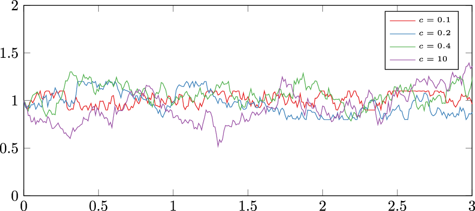
Figure 3. Zoomed-in version of Figure 2.
4 Software tool and computational results
4.1 Software tool
For the computations, we use the network simulation tool grazer Footnote 3 written in C++. It is an open source software suite developed at the Chair of Scientific Computing at the University of Mannheim. For the purpose of long-term usability, the following design goals have been chosen:
-
Easy installation
-
Full C++17-standard compliance with tested support for compilers GCC-9+, Clang-9+ and Visual Studio 2019+ (Other compilers are probably easy to use because of the standard compliance.)
-
Few external dependencies
-
High test coverage
-
Clean warning profile
-
Open Source License (AGPL 3.0).
The dependencies we have are Eigen, see [Reference Guennebaud and Jacob29], N. Lohmanns json library,Footnote 4 googletest,Footnote 5 pcg-random, see [Reference O’Neill43] and CLI11. Footnote 6
4.1.1 Installation
In order to build grazer, you need three pieces of software: CMake,Footnote 7 GitFootnote 8 and a C++17 capable C++ compiler, for example clang,Footnote 9 gccFootnote 10 or msvc.Footnote 11 Installation can be done by executing
Listing 1: Installation
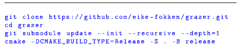
Afterwards there is a grazer binary in …/grazer/release/src/Grazer called grazer or grazer.exe (on Windows).
4.1.2 Usage
Up to now, grazer is a command line application usable from any shell convenient, that is controlled by a number of input json files. In the medium term future, it is planned to also support a python interface.
Grazer is used by pointing it to a directory with input json files.
Listing 2: Calling grazer
for example will run the problem defined in the directory data/one pipeline. The problem directory contains a subdirectory problem, which holds the json files problem data.json, topology.json, boundary.json, initial.json and control.json. Note that the layout of topology.json was heavily inspired by the layout of GasLib files, see [Reference Schmidt49].
After solving the problem, an output file will be generated in data/one pipeline/output. This again a json file, so it can be read with almost all software. For ease of use, some helper programs, compiled alongside grazer, can be found in release/helper functions/. For example calling
Listing 3: Calling grazer
will extract the json data into a csv file for usage with plotting tools. Helpers that import these into native formats of python are planned.
In addition, json schemas can be generated and inserted into the jsons (Up to now with the exception of problem data.json) with
Listing 4: Calling grazer
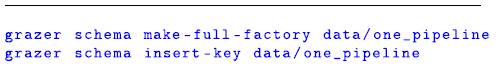
This has the advantage that json-aware editors help the users to only write jsons that are valid inputs for grazer which cuts down on bug searches.
As a final note on the usage, be aware that although grazer runs only sequentially, the output filename is chosen ’atomically’, meaning that two instances of grazer running in parallel will not interfere with each other’s output. This is especially useful when executing many runs of stochastic problems in a Monte-Carlo method as was done in the present work.
Note that parts of the API are still subject to change. For an up-to-date explanation, check out the userguide in docs/userguide.tex in the repository.
4.1.3 A rough overview of the inner workings
On execution, grazer will read those files, configure the Newton solver according to settings in problem data.json, construct a representation of the network from topology.json, set initial and boundary values from the respective files and then start solving the problem time step per time step. In each time step, the model equations and their derivatives described above are evaluated to find a solution of them with Newton’s method. If successful, the solution is saved and the next time step is started. If no solution can be found, the user is notified and all data computed in prior time steps are written to the output files. If all time steps can be solved, all data are written out.
If a stochastic component is present in the network, a pseudo random number generator must be initialised with a seed. These are generated automatically or taken from the boundary.json file, if a seed is present in there.
4.1.4 Optimisation
Grazer is also capable of computing optimal controls. To this end, certain components in a network can supply cost and constraint functions as well as their first derivatives. This information together with derivatives of the model equations with respect to states and controls is transformed via the adjoint method (see e.g. [Reference Kolb36] for an explanation) into derivatives with respect to the controls only. The latter are then handed over by grazer to IPOPT (see [Reference Wächter and Biegler52]), that actually computes the optimal controls. In our trials, we have used the linear solver MUMPS (see [Reference Amestoy2, Reference Amestoy3]), yet any other solver that can be interfaced with IPOPT could be used. Note that no second derivatives are provided by grazer, which means that for the optimisation only quasi-Newton methods are available. A short example of this optimisation is provided at the end of this work. It is probably noteworthy that grazer is capable of handling constraint and control discretisations, that are coarser than the state discretisations detailed in Section 3. This is done by evaluating constraints only every nth time step, where n can be chosen by the user. Of course, this can lead to constraint violations in between and therefore any such solution should be checked for such an occurrence. The coarser control discretisation is instead handled by interpolating controls linearly between two control discretisation points.
4.2 Scenario description
Here we describe the considered scenario of a combined power and gas network. All data can be found in the git repo https://github.com/eike-fokken/efficient_network-data.git.
4.3 Specification of the power network
As starting point for the power network, we use the ieee-300-bus system, as given in the Matpowercase (see [Reference Zimmerman, Murillo-Sanchez, Thomas and Syst56]) case300. It is a power network of 69 generator nodes, 231 load nodes and 411 transmission lines. We alter the ieee-300 network in the following way.
-
The power demand (real and reactive) is lowered by 10%.
-
The former slack node N7049 is changed into a PV-node.
-
The old PV-nodes given in table Table 3 are turned into slack busses (V
$\phi$
-nodes). -
All PQ-nodes are turned into stochastic PQ-nodes described in Section 2.4 and Section 3.5.

At the new V $\phi$
-nodes, power that is generated from gas burned in gas power plants is injected into the power network according to equation (2.15). A picture of our power network can be found in Figure 4.
$\phi$
-nodes, power that is generated from gas burned in gas power plants is injected into the power network according to equation (2.15). A picture of our power network can be found in Figure 4.

Figure 4. Power network with green gas power plants, blue non-gas power plants and red loads.
4.4 Specification of the gas network
As starting point for the gas network we use the GasLib-134 system (see [Reference Schmidt49]). A picture an be found in Figure 5.
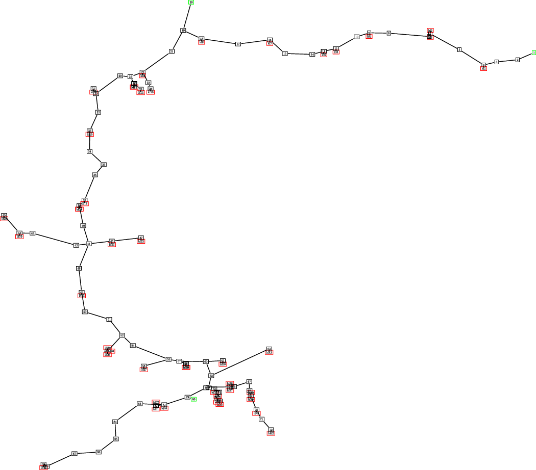
Figure 5. The gas network with green sources, red sinks and black junctions.
It is a gas network of 86 pipelines, 3 inflow nodes (sources) and 45 outflow nodes (sinks). The inflow of gas remains constant over time and is given in Table Table 2.
Table 2. Inflow into the gas network
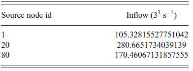
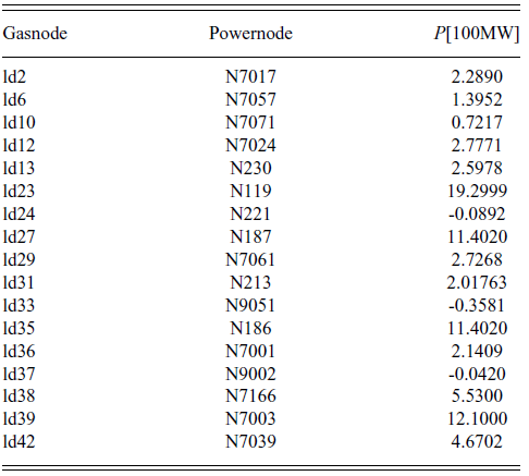
Here, 17 of the sinks, all gathered in table Table 3, draw gas to be converted into power. The amount is set by the power network and is computed from the PF equations. All other sinks do not consume gas.
Table 3. Start and end nodes of gas power conversion plants and the deterministic demands of real power
4.5 Specification of the Gas Power connections
The two networks are connected through gas power conversion plants, that turn gas into power, when power is needed and power into gas, when surplus power is available. The gas power conversion plants are arcs between the nodes listed in Table 3. For simplicity, they all share the same efficiencies both for power generation and gas generation, namely they have
 \begin{equation} \begin{aligned} E_{\text{PtG}} &= 43.56729\ \mathrm{MW}\ \mathrm{s\ m}^{-3} \\ E_{\text{GtP}} &= 12.56\ \mathrm{MW}\ \mathrm{s\ m}^{-3} . \end{aligned}\end{equation}
For the smoothing constant, we choose $\kappa = 60\ \mathrm{m}^{3} \mathrm{s}^{-1}$
. As
$\kappa = 60\ \mathrm{m}^{3} \mathrm{s}^{-1}$
. As $\kappa$
has no role but to mollify the kink in the switching from one conversion to the other, the choice is purely driven by numerical factors. The choice of
$\kappa$
has no role but to mollify the kink in the switching from one conversion to the other, the choice is purely driven by numerical factors. The choice of $\kappa$
must depend on the time step size, where smaller time steps allow for smaller
$\kappa$
must depend on the time step size, where smaller time steps allow for smaller $\kappa$
and therefore more sudden switching behaviour.
$\kappa$
and therefore more sudden switching behaviour.
All further data concerning these plants is gathered in Table 3. There a real power demand is also given, which corresponds to the default demand in our setting, when no uncertainty is present.
4.6 Specification of the stochastic power demand nodes
As mentioned, all PQ-nodes of the ieee-300-bus system are replaced by stochastic PQ-nodes. As mean function, we choose the power demands given by the ieee-300-bus problem, but lowered by 10%. In addition, we choose for the drift coefficient $\theta = 3 $
, for the stability constraint we choose
$\theta = 3 $
, for the stability constraint we choose
 \begin{equation} \Delta t_{\text{stoch}} = \frac{0.1}{\theta},\end{equation}
which results in rather high numbers of stochastic time steps but is unfortunately needed for convergence. For the cut-off, we use $c = 0.4$
. The diffusion coefficient
$c = 0.4$
. The diffusion coefficient $\sigma$
will be varied to compare different values.
$\sigma$
will be varied to compare different values.
4.7 Computational results
In each run, we simulate the combined network over the course of $24 \mathrm{h}$
(86,400 s) with a time stepsize of
$24 \mathrm{h}$
(86,400 s) with a time stepsize of $0.5 \mathrm{h}$
(
$0.5 \mathrm{h}$
( $1800\ \mathrm{s}$
).
$1800\ \mathrm{s}$
).
4.7.1 Steady state vs. stochastic example
At first, we simulate the network in a deterministic setting, which can be achieved by setting $\sigma$
in (3.3) to zero. To keep the scenario simple, we choose steady state initial conditions, which were generated by using arbitrary initial conditions and integrating them for a long time. The resulting end state is then used as initial conditions for our setting.
$\sigma$
in (3.3) to zero. To keep the scenario simple, we choose steady state initial conditions, which were generated by using arbitrary initial conditions and integrating them for a long time. The resulting end state is then used as initial conditions for our setting.
In this deterministic setting, we find the (constant) power demands in the gas plants given in Table 3. To illustrate our results, we will usually picture the situation of pipe p_br71, which is located to the lower right in Figure 5 connecting nodes 71 and 72. The steady state solution in pipe p_br71 remains constant over time as is fitting for a steady state solution. The same is true for the flow and also for all other pipes in the network.
Along with the deterministic setting, we simulate a scenario with $\theta = 3.0$
and
$\theta = 3.0$
and $ \sigma=0.45$
for all PQ-nodes. The number of stochastic steps is set to at least 1000 which, due to stability constraints mentioned in (3.5), was then automatically raised to 18,000.
$ \sigma=0.45$
for all PQ-nodes. The number of stochastic steps is set to at least 1000 which, due to stability constraints mentioned in (3.5), was then automatically raised to 18,000.
A comparison of the steady state and stochastic pressure can be seen in Figure 6 while a comparison of the fluxes is given in Figure 7.

Figure 6. Pressure evolution in p_br71 for deterministic and some realisations of stochastic demand.

Figure 7. Flow evolution in p_br71 for deterministic and some realisations of stochastic demand.
In the power network, we find for the PQ-node N1 power demands over time like those in Figures 8 and 9. Of course the situation is similar for all PQ-nodes.

Figure 8. Real power demand in N1 for deterministic and stochastic demand with $\sigma =0.45$
.
$\sigma =0.45$
.

Figure 9. Reactive power demand in N1 for deterministic and stochastic demand with $\sigma =0.45$
.
$\sigma =0.45$
.
4.7.2 Stochastic demand with variable noise
Now we examine repercussions of the uncertainty on the gas network. Therefore, we make 100 runs for each $\sigma \in \{0.05,0.1,0.3,0.45\}$
and compare the quantiles at 50%, 75% and 90%. Taking an arbitrary point in time,
$\sigma \in \{0.05,0.1,0.3,0.45\}$
and compare the quantiles at 50%, 75% and 90%. Taking an arbitrary point in time, $t = 12\ \mathrm{h}$
, the quantiles for the pressure can be seen in Figure 10.
$t = 12\ \mathrm{h}$
, the quantiles for the pressure can be seen in Figure 10.

Figure 10. Comparison of pressure quantile boundaries at different $\sigma$
at
$\sigma$
at $t = 12\ \mathrm{h}$
in pipeline p_br71.
$t = 12\ \mathrm{h}$
in pipeline p_br71.
For the flow the quantile comparison can be found in Figure 11.

Figure 11. Comparison of flow quantile boundaries at different $\sigma$
at
$\sigma$
at $t = 12\ \mathrm{h}$
in pipeline p_br71.
$t = 12\ \mathrm{h}$
in pipeline p_br71.
For both quantities, we see the expected expansion of quantile boundaries with higher diffusion $\sigma$
.
$\sigma$
.
4.7.3 Comparison of deterministic and stochastic pressure prediction
Now we give an overview of the impact of the volatility in power demand on the network. Therefore, we revisit the scenario with the highest volatility, that is with $\sigma = 0.45$
and consider again a time frame of
$\sigma = 0.45$
and consider again a time frame of $24\ \mathrm{h}$
. In Figure 12 one can see the maximal deviation of real power demand from the steady state solution. At first glance, this looks similar to Figure 4, just with colours cycled around. This is due to the fact, that the load nodes have defined volatility as they follow their own Ornstein-Uhlenbeck process approximation defined in equation (3.3). The PV-nodes on the other hand have zero volatility in real power. Yet the V
$24\ \mathrm{h}$
. In Figure 12 one can see the maximal deviation of real power demand from the steady state solution. At first glance, this looks similar to Figure 4, just with colours cycled around. This is due to the fact, that the load nodes have defined volatility as they follow their own Ornstein-Uhlenbeck process approximation defined in equation (3.3). The PV-nodes on the other hand have zero volatility in real power. Yet the V $\phi$
-nodes must account for all remaining power demand and as such have the highest volatility. A similar picture can be found in Figure 13, where the deviation of the reactive power is depicted. Here the PV-nodes do not have zero volatility, yet it seems that they also do not carry much volatility in Q.
$\phi$
-nodes must account for all remaining power demand and as such have the highest volatility. A similar picture can be found in Figure 13, where the deviation of the reactive power is depicted. Here the PV-nodes do not have zero volatility, yet it seems that they also do not carry much volatility in Q.

Figure 12. Heatmap of the maximal real power deviation over the course of $24\ \mathrm{h}$
, units are in
$24\ \mathrm{h}$
, units are in $100\ \mathrm{MW}$
.
$100\ \mathrm{MW}$
.

Figure 13. Heatmap of the maximal reactive power deviation over the course of $24\ \mathrm{h}$
, units are in
$24\ \mathrm{h}$
, units are in $100\ \mathrm{MW}$
.
$100\ \mathrm{MW}$
.
At last, we consider the possible impact of the volatility in the power network on the gas network. Therefore, we show the maximal pressure deviation from the steady state solution over the course of $24 \mathrm{h}$
for
$24 \mathrm{h}$
for $\sigma = 0.45$
in Figure 14. It is easily seen that the lower part of the network experiences much higher pressure volatility than the upper part. This is expected, as on the one hand the upper part has higher pressure as the three gas sources are located there and on the other hand many more gas power conversion plants are located in the lower part, so that the volatility can add up.
$\sigma = 0.45$
in Figure 14. It is easily seen that the lower part of the network experiences much higher pressure volatility than the upper part. This is expected, as on the one hand the upper part has higher pressure as the three gas sources are located there and on the other hand many more gas power conversion plants are located in the lower part, so that the volatility can add up.

Figure 14. Heatmap of the maximal pressure deviation over the course of $24\ \mathrm{h}$
, units are in bar.
$24\ \mathrm{h}$
, units are in bar.
4.7.4 Optimisation example
Finally, we show results of an optimisation task carried out with grazer. The Gaslib-134 network actually contains two controllable components, a compressor between the nodes $29/30$
and a control valve between the nodes
$29/30$
and a control valve between the nodes $65/66$
. We take the steady state solution from above but add two continuous constraints in order to make the controllable components actually do some work. At the sink ld_22, we impose a lower pressure bound of
$65/66$
. We take the steady state solution from above but add two continuous constraints in order to make the controllable components actually do some work. At the sink ld_22, we impose a lower pressure bound of $70 \mathrm{bar}$
at
$70 \mathrm{bar}$
at $t=0$
,
$t=0$
, $90 \mathrm{bar}$
at
$90 \mathrm{bar}$
at $t= 24\ \mathrm{h}$
and interpolate linearly in between. In addition, we impose an upper pressure bound at sink ld_40 of
$t= 24\ \mathrm{h}$
and interpolate linearly in between. In addition, we impose an upper pressure bound at sink ld_40 of $90 \mathrm{bar}$
at
$90 \mathrm{bar}$
at $t=0$
,
$t=0$
, $70\ \mathrm{bar}$
at
$70\ \mathrm{bar}$
at $t= 24\ \mathrm{h}$
and again interpolate linearly in between. As cost function we choose
$t= 24\ \mathrm{h}$
and again interpolate linearly in between. As cost function we choose
 \begin{eqnarray*} \int_0^{24}\ \mathrm{h}u_{\text{compressor}}(t)^2\mathrm{d}t,\end{eqnarray*}
so that using the valve is free but compressor costs should be minimised. The control is discretised with the same discretisation already used by the states, yielding 49 time points. Also, the constraints are evaluated at every state time step. While grazer is capable of using coarser resolutions of both constraints and controls, the problem at hand is small enough to compute a solution in approximately a minute on a workstation. Using only 11 controls cut this time in half. In addition, evaluating the constraints only every fifth step reduces the time again by half. The control of the valve is constrained to not exceed $40\ \mathrm{bar}$
to keep the optimisation routine from trying controls that are too high to yield a solution of the simulation. The compressor control is capped at
$40\ \mathrm{bar}$
to keep the optimisation routine from trying controls that are too high to yield a solution of the simulation. The compressor control is capped at $120\ \mathrm{bar}$
, although this bound is never attained.
$120\ \mathrm{bar}$
, although this bound is never attained.
With this data grazer computes the optimal controls in Figures 15 and 16. The compressor control in Figure 15 nicely ramps up as the lower pressure bound in ld_22 rises. On the other hand, the valve control in Figure 16 stays at zero until this is not sufficient anymore to satisfy the decreasing upper pressure bound in ld_40 at which point the control rises up to the maximal value, staying there until the end. As the valve control incurs no cost, this is one of many possible configurations.

Figure 15. Computed optimal control of the compressor at nodes $29/30$
.
$29/30$
.

Figure 16. Computed optimal control of the valve at nodes $65/66$
.
$65/66$
.
A comparison of pressure evolution at the two sinks ld_22 and ld_40 is given in Figures 17 and 18. It can be seen that the compressor increases the pressure just enough to satisfy the lower pressure bound as its usage is penalised, while the (free to use) valve at first matches the upper pressure bound exactly but later on over-compensates it rather strongly.

Figure 17. Comparison of controlled and uncontrolled pressure at ld_22.

Figure 18. Comparison of controlled and uncontrolled pressure at ld_40.
5 Summary and future work
We introduced the new open source software tool grazer that can be used to efficiently simulate numerical problems that are defined on networks. We used grazer to simulate a coupled gas and power network with uncertain power demand presented repercussions of the uncertain power demand within the gas network.
Future work includes the extension of grazer to more complex optimisation problems and other types of uncertainty.
Acknowledgments
The authors acknowledge support through the BMBF project ENets (05M18VMA) and 320021702/GRK2326, 333849990/IRTG-2379 and DFG HE5386/18-1 and DFG HE5386/23-1.


 Open access