When assessing the transmissibility of an infectious disease, it is important not only to measure the overall transmission potential [Reference Greenwood1], but also the illness-stage dependent infectiousness [Reference Hope-Simpson2] to understand and clarify the effectiveness of control strategies. Transmission potential on a whole has been measured by the basic reproduction number, R ₀, i.e. the average number of secondary cases arising from the introduction of an index case into a fully susceptible population [Reference Dietz3, Reference Diekmann and Heesterbeek4]. Since a reproduction number <1 indicates the eventual termination of an outbreak based on a threshold theorem, the knowledge of R ₀ has been extremely useful in determining the required vaccination coverage and clarifying ecological and public health questions (e.g. periodicity of epidemics, average age at infection and heterogeneous transmissions) based on population dynamics [Reference Anderson and May5]. For simplicity, infectiousness is frequently assumed to be constant [Reference Becker6] and thus, the frequency of secondary transmissions by disease age (i.e. the time since onset of the disease) has rarely been evaluated. One of the rare exceptions is HIV infection whose infectiousness has been evaluated with regard to disease age, based on statistical analysis of partner studies [Reference Shiboski and Jewell7]. The results suggest that the infectiousness of HIV is not constant, and this could largely influence the qualitative patterns of the epidemic [Reference Diekmann and Heesterbeek4, Reference Koopman8]. The knowledge of the disease-age-specific infectiousness is not only crucial for slowly progressing diseases but also for acute directly transmitted diseases, where targeted control measures, including isolation and contact tracing, have to be implemented as early as possible during the infectious period, and thus, their effectiveness largely depends on the time-course of infectiousness [Reference Fraser9, Reference Eichner10].

One approach was to quantify how the pathogen load changes over time by using the most sensitive microbiological techniques (e.g. real-time polymerase chain reaction) [Reference Chu11], but such observations are practically limited to the time after onset of symptoms and the pathogen load information can only be a useful measure of infectiousness if it is correlated with actual transmission. With regard to smallpox, several attempts have been made to measure the distribution of the virus-positive period [Reference Downie12, Reference Sarkar13]. Despite rigorous studies, sample sizes were limited and, in particular, few samples could be obtained during the early stage of illness. Due to different laboratory techniques, the obtained viraemic periods differ widely. In this paper, we propose an epidemiological evaluation method, based on the distribution of the incubation period and the transmission network (who infected whom), to estimate how smallpox infectiousness varies over the course of illness.

The key information used in our approach includes the distribution of the incubation period and the transmission network. The incubation period, denoted by τ, is the time from infection to onset of disease (i.e. fever). The distribution has been fitted to a lognormal distribution, f(τ|μ, σ), with the maximum-likelihood estimates of the mean and the standard deviation (s.d.) of log (τ) being μ=2·47 and σ=0·17, respectively (Fig. 1a; H. Nishiura & M. Eichner, unpublished observations). The transmission network is the observed chain of transmission that yields the information of who infected whom. This type of information has already been explored to assess the number of secondary transmissions over the course of an epidemic [Reference Haydon14] and to evaluate individual variations in transmission [Reference Lloyd-Smith15, Reference Nishiura16], but it also enables us to obtain the serial interval, i.e. the time from symptom onset in a primary case to symptom onset in a secondary case [Reference Fine17, Reference Wallinga and Teunis18]. This study uses observed serial intervals in five smallpox outbreaks, in Glasgow (1950), Brighton (1950–1951), Industrial Pennines (1953), Bawku (1967) and Calcutta (1971–1972) [Reference Laidlaw and Horne19–Reference Mukherjee, Sarkar and Mitra23]. A total of 223 serial intervals were identified. The mean (and median and s.d.) of these intervals was 16·0 (16·0 and 4·0) days. The minimum and maximum intervals were 6 and 37 days, respectively.

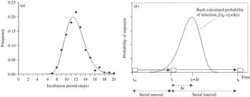
Fig. 1. Distribution of the incubation period and illustration of the estimation procedure. (a) Observed (◆) and fitted (—) lognormal distribution of the incubation period (n=379; H. Nishiura & M. Eichner, unpublished observations). (b) Back-calculation of the transmission probability: case m infected case l who subsequently infected case k. Their times of onset are t _m, t _l and t _k, respectively. Using the difference of the disease onset (serial interval) t _k−t _l together with the distribution of the incubation period, the disease-age-specific probability of transmission from case l to case k is obtained. □, Onset of cases;, transmission.

Figure 1b illustrates our estimation method using a chain of transmission of three consecutive cases, m, l and k. Based on observation, it is known that case m infected case l who subsequently infected case k. We denote the times of onset of these cases by t _m, t _l and t _k, respectively, where t _k – t _l is the serial interval between cases l and k. Using this interval together with the distribution of the incubation period, the disease-age-specific infectiousness of case l is obtained. Assuming that the probability of observing transmission from primary case l to the secondary case k for each day can be extracted from the independently identically distributed incubation period, the probability density that case k was infected Δt days after onset of case l is given by:

(1)

Transmission from case l to k may have occurred before the onset of case l. Although one could consider any time of transmission dating back to t _m, we restrict the potentially contagious period to x=5 days before onset of primary case l. As the incubation period lasts longer than 5 days in over 99·9% of cases, this assumption does not create major conflicts (e.g. we do not observe transmission from case l to k before m infected l). Some secondary cases were vaccinated before exposure or received post-exposure vaccination, but we assume that their vaccination did not significantly influence the length of the incubation period, because the cases did develop smallpox. Since the parameters of the incubation period distribution are known, eqn (1) can numerically be solved by discrete approximation of the incubation period distribution. Other underlying assumptions include the following: (i) the frequency of secondary transmission is independent of the overall transmission potential; although the contagiousness of vaccinated cases might have been lower than that of unvaccinated ones, we assume that their relative contagiousness in the different phases of disease was that of unvaccinated cases, (ii) human behaviour, spatial information and extrinsic factors (i.e. the implementation of control measures) can be ignored (for discussion on this point see below).

Using these assumptions, the disease-age-specific infectiousness can be estimated by using a likelihood-based procedure. We denote the number of observed serial intervals of length t by s(t). Let λ(u) denote the number of secondary transmissions occurring u days after the onset of the primary case (including the days for u<0). We then obtain the expected number of serial intervals of length Δt by the convolution equation:

(2)

where k(i) denotes the secondary cases infected by case i. The basic idea of eqn (2) can now be linked to the method of back-calculation in HIV/AIDS [Reference Brookmeyer and Gail24]. Since we assume the incubation period distribution to be known, estimates of disease-age-specific infectiousness can be obtained in a non-parametric fashion [Reference Becker, Watson and Carlin25] assuming a step function model for λ(u):

(3)

Further details are given in the Appendix.

Figure 2a shows the estimated daily frequency of secondary transmissions with corresponding 95% confidence intervals (CI) based on the profile likelihood. Between 3 and 6 days after onset of fever, which roughly corresponds to the time immediately after the onset of rash, the daily frequency of secondary transmissions was highest, yielding 20·6% (95% CI 15·1–26·4) of the total number of secondary transmissions. Expected cumulative frequencies of secondary transmissions before onset of fever and up to 3 days after onset of fever were 2·6% and 23·7%, respectively. The obtained estimates suggest that 91·1% of all secondary transmissions occurred up to 9 days after onset of fever. Figure 2b compares the observed and predicted serial intervals. Figure 2b confirms a relatively good overall agreement between predicted and observed data, but the χ² goodness-of-fit test revealed a significant deviation between the observed and expected serial intervals (see legend for Fig. 2), which is largely attributable to outliers in the observed data.

Fig. 2. Frequency of secondary transmissions and predicted serial intervals. (a) Expected daily frequency of secondary transmissions with corresponding 95% confidence intervals (CI) (—, upper 95% CI; —, expected; ….., lower 95% CI). Disease age t=0 denotes the onset of fever. (b) Observed (□) and predicted (■) daily counts of the serial intervals (n=223). The χ² test revealed significant deviation between the observed and predicted values (χ²₅=20·9, P<0·01). When assessing the goodness-of-fit of our models, using the χ² statistic, we divided the serial interval into ten groups (⩽11, 12–13, 14–15, 16–17, 18–19, 20–21, 22–23, 24–25, 26–27 and ⩾28 days).

The significance of estimating disease-age-specific infectiousness of smallpox lies in the practical implications both on the population and the individual level. Previous studies frequently assumed a deterministic (fixed) incubation period of 11 or 12 days to infer the date of smallpox infection [Reference Rao26, Reference Mack27]. As isolation of cases is critically important to control smallpox [Reference Fraser9, Reference Eichner10], it is crucial to evaluate the time at which isolation can be delayed. Our estimates are also useful for the evaluation of surveillance containment measures (i.e. ring vaccination) where the disease-age-specific infectiousness plays a key role [Reference Kretzschmar28]. Our study implies that isolation could be extremely effective if performed before onset of rash and that delayed isolation of symptomatic cases could still be effective if performed within a few days after onset of rash. The highest infectivity immediately after onset of rash is consistent with previous suggestions based on observational experience [Reference Downie12, Reference Sarkar13, Reference Fenner29].

This paper proposes a simple method to estimate the disease-age-specific infectiousness. So far, similar information for an acute infectious disease has only been obtained in a rigorous study based on longitudinal data of household transmissions of influenza using Markov chain Monte Carlo [Reference Cauchemez30]. Our study shows that the incubation period and precise data on who infected whom enables the estimation of the infectiousness without specific settings such as households. The proposed method is extremely useful as far as independence of transmission during the course of disease can be assumed for diseases with acute course of illness. (Note: this assumption is not recommended for slowly progressing diseases such as HIV/AIDS [Reference Wallinga and Teunis18].) However, the probability of transmission tends to be biased by various factors: our small sample of serial intervals may have been influenced by local factors such as differences in contact behaviour and mobility of cases. This partly explains why several outliers are observed in the serial intervals (Fig. 2b). For example, Fig. 3 shows the total number of cases who contributed to the generation of secondary cases (based on serial intervals) and the subset of those who were admitted to the hospital before onset of the secondary cases in Brighton during 1950–1951 [Reference Cramb20]. Other data sources hardly provided us with similar information. The impact of isolation, which could not be explicitly incorporated in this study due to small sample sizes, can be assessed by looking at the area under the dotted line (Fig. 3). Thus, the infectiousness several days after appearance of rash may have been underestimated. This could partly explain a disagreement with a previous study [Reference Eichner and Dietz31] in which the infectiousness during the prodromal period was estimated as 8·2% of the overall transmission potential. In conclusion, this study showed a simple back-calculation of infectiousness by disease age, based on the known distribution of the incubation period distribution and the transmission network.

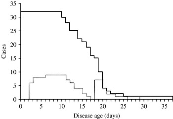
Fig. 3. Number of infectious cases and those isolated among them by disease age. The solid line shows how many index cases were followed by secondary cases t days after onset of symptoms and had to be considered as still being infectious in Brighton (1950–1951). The dotted line shows how many of these index cases were hospitalized on the given disease age.

APPENDIX: Likelihood-based approach

Since the serial interval is given with a daily precision, we consider the convolution eqn (2) in discrete time:

(A1)

where f _k is the probability that the incubation period has length k days. Assuming that λ_u is generated by a non-homogeneous Poisson process, resulting in s _t serial intervals of length t, the likelihood function, which is needed to estimate λ_u, is proportional to

(A2)

where r _t denotes the daily counts of the serial interval (Fig. 2b). The maximum-likelihood estimates of λ_u were obtained by minimizing the negative logarithm of eqn (A 2). The 95% CI was determined using the profile likelihood.