


Impact Statement
Climate indicators are important covariates on several research fields, but datasets directly compatible with administrative boundaries in Brazil are scarce and not available for long time spans. We propose consistent dataset of climate indicators for the Brazilian municipalities derived from the ERA5-Land project, covering the period from 1950 to 2022.
1. Introduction
Climate variables are commonly used as covariates in statistical modeling on research fields like agriculture, public health, and economics, as climate trends affect several biological and physical processes (Overpeck et al., Reference Overpeck, Meehl, Bony and Easterling2011).
Climate indicators can be obtained by direct measurement, taken in place by a set of different equipment like weather stations and rain gauges, or by indirect measurement, with artificial satellites and remote sensing. The usage of in situ data is usually limited in space by the uneven distribution of sensors and in time considering the starting date of data recording and possible gaps due to technical problems and other reasons. In Brazil, weather stations are unequally scattered over the territory and limited in number due to implementation and maintenance costs and also present data with different time spans and significant gaps for some locations. Statistical interpolations in time and space from weather stations data are often used to infer the weather indicators on areas and time intervals that were not covered by sensors (de Aguiar and Lobo, Reference de Aguiar and Lobo2020).
In order to improve the availability of climate indicators in longer time spans and more refined spatial scales, data assimilation techniques have been developed and applied to produce climate reanalysis, which can be defined as the “consistent reprocessing of archived weather observations using a modern forecasting system” (Dee et al., Reference Dee, Balmaseda, Balsamo, Engelen, Simmons and Thépaut2014). By this approach, observations from multiple sources of direct and indirect climate measurements are combined with methodological procedures for calibration, correction, and cross-validation with field data (Funk et al., Reference Funk, Peterson, Landsfeld, Pedreros, Verdin, Shukla, Husak, Rowland, Harrison, Hoell and Michaelsen2015; Abatzoglou et al., Reference Abatzoglou, Dobrowski, Parks and Hegewisch2018; Muñoz-Sabater et al., Reference Muñoz-Sabater, Dutra, Agustí-Panareda, Albergel, Arduini, Balsamo, Boussetta, Choulga, Harrigan, Hersbach, Martens, Miralles, Piles, Rodríguez-Fernández, Zsoter, Buontempo and Thépaut2021) to produce models that are able to retrospectively infer climate variables on global scale.
Climate reanalysis products provide continuous data with regular sets of indicators for long time spans and wide spatial coverage. The exceptional continuity and integrity make reanalysis products widely applied in some research fields, as hydrological reanalysis. On this specific use case, indicators are computed to coherent register water resource indicators on long time spans and large territorial areas, as the Brazilian basin (Wongchuig et al., Reference Wongchuig, De Paiva, Siqueira and Collischonn2019; Zou et al., Reference Zou, Lu, Jiang, Qin, Yao, Xin and Su2022).
The approaches for measuring and registering weather indicators usually result in large datasets of different formats and extensions with multiple time and spatial resolutions, presenting a multitude of indicators covering extensive portions of territory in time series formats. This imposes a challenge to some research fields like economics and public health, where statistical modeling is carried out by using lattice structures (Cressie, Reference Cressie1991; Morgenstern, Reference Morgenstern1995). Those models employ aggregated data representing groups or geographical regions, like the total number of disease cases in a region or the average income of a neighborhood. Administrative spatial boundaries like countries, states, counties, and municipalities are some examples of lattice aggregation used in those models.
Considering the continuous nature of weather data, one common solution to introduce weather variables into lattice models is to aggregate weather indicators to the same lattice structure as the other variables present in the model. An example would be the modeling of dengue disease spread over administrative health regions: the number of dengue disease cases is usually presented in aggregated form, by the sum of confirmed cases in a health region. Thus, spatially continuous variables used as predictors of dengue disease, such as temperature and precipitation, must be aggregated to the same region’s boundaries of the dengue case. An application of this approach can be found in the study by Lowe et al. (Reference Lowe, Cazelles, Paul and Rodó2016).
In order to summarize gridded climate indicators into boundary lattice structures, zonal statistics can be used. Zonal statistics are descriptive statistics calculated using the set of cells that spatially intersect a given boundary (Tomlin, Reference Tomlin1994). For each boundary in a map of regions, statistics like average, maximum value, minimum value, standard deviation, and others are computed to statistically represent the cells that intersect the boundary. This is illustrated by Figure 1.
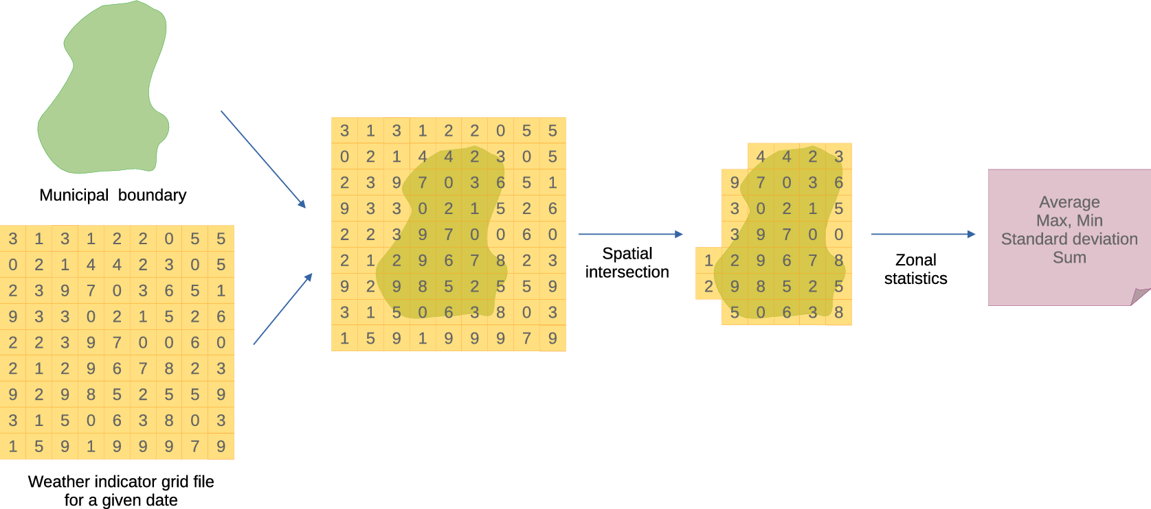
Figure 1. Zonal statistics operation.
The zonal statistical indicators may also be weighted by the proportion of the cell that overlays the geographical boundaries and by other layers, as will be further explored. This work proposes the adoption of the ERA5-Land climate reanalysis to compute zonal statistics in order to provide climate indicators for the Brazilian municipalities for a long time span.
1.1. Related works
Similar procedures to summarize climate indicators for Brazilian municipalities have been done in other projects. The SISAM project (INPE, 2019) created a dataset with weather and air pollution indicators for Brazilian municipalities, with daily data from January 1, 2000, to December 31, 2019. Different data sources with different spatial resolutions for specific periods were used in this project. The ERA-Interim is used as a source but is currently supplanted by the newer ERA5-Land reanalysis (Muñoz-Sabater et al., Reference Muñoz-Sabater, Dutra, Agustí-Panareda, Albergel, Arduini, Balsamo, Boussetta, Choulga, Harrigan, Hersbach, Martens, Miralles, Piles, Rodríguez-Fernández, Zsoter, Buontempo and Thépaut2021), limiting its utilization. The adopted methodology to create climate indicators for municipalities consisted of observing the data exclusively on the cell where the municipality city hall geographical coordinates are spatially located. This punctual observation, however, does not generalize to the municipality’s territorial extension.
Abdalla et al. (Reference Abdalla, Augusto, Chame, Dufek, Oliveira and Krempser2022) present datasets for Brazilian municipalities with different temporal resolutions and temporal coverages, including temperature and precipitation aggregated by the year, from 1981 to 2020. The adoption of yearly weather aggregation limits its usage.
It is also important to point that similar procedures are performed punctually as a methodological step by some researches to compute climate indicators on limited time spans to specific Brazilian municipalities or other boundaries in different countries (Lowe et al., Reference Lowe, Bailey, Stephenson, Graham, Coelho, Sá Carvalho and Barcellos2011; Schneider et al., Reference Schneider, Sebastianelli, Spiller, Wheeler, Carmo, Nowakowski, Garcia-Herranz, Kim, Barlevi, El Raiss Cordero, Liberata Ullo, Mathieu and Lowe2021; Abdalla et al., Reference Abdalla, Augusto, Chame, Dufek, Oliveira and Krempser2022). Usually, the adopted methodology is short described in the published papers and not directly reproducible. To the best of the authors’ knowledge, there are no similarly published studies focusing on the usage of zonal statistics to compute climate indicators with climate reanalysis products. Therefore, there is still a demand for research to produce climate indicators ready-to-use for lattice modeling, aggregated at the municipal level in Brazil and other countries at daily resolution, covering a long time span.
This paper aims to propose a methodology to compute climate indicators aggregated by delimited spatial boundaries, such as administrative limits, with a Brazilian use case adopting the ERA5-Land reanalysis (Muñoz-Sabater et al., Reference Muñoz-Sabater, Dutra, Agustí-Panareda, Albergel, Arduini, Balsamo, Boussetta, Choulga, Harrigan, Hersbach, Martens, Miralles, Piles, Rodríguez-Fernández, Zsoter, Buontempo and Thépaut2021) as a data source in order to produce daily zonal statistics of climate indicators for Brazilian municipalities from 1950 to 2022.
The proposed methodology may be later applied to other spatial limits in Brazil (other administrative boundaries and hydrological basins, for example) and other countries. The availability of ready-to-use climate indicator datasets has the potential to ease the work of research groups of several areas, not requiring specific knowledge of Geographic Information Systems, climate data processing, and other fields, enabling them to focus on modeling and its main research objectives.
2. Methods
2.1. Data sources
The exceptional continuity and integrity over long time spans present on climate reanalysis products make them good candidates for the creation of zonal statistics indicators, offering stable indicator definitions, methodology, and availability for several years and for large territorial areas such as the Brazilian territory.
The European ReAnalysis product, created by the European Centre for Medium-Range Weather Forecasts (ECMWF) with the Copernicus Climate Change Service (C3S), is on its fifth generation (ERA5, Hersbach et al., Reference Hersbach, Bell, Berrisford, Hirahara, Horányi, Muñoz-Sabater, Nicolas, Peubey, Radu, Schepers, Simmons, Soci, Abdalla, Abellan, Balsamo, Bechtold, Biavati, Bidlot, Bonavita, De Chiara, Dahlgren, Dee, Diamantakis, Dragani, Flemming, Forbes, Fuentes, Geer, Haimberger, Healy, Hogan, Hólm, Janisková, Keeley, Laloyaux, Lopez, Lupu, Radnoti, de Rosnay, Rozum, Vamborg, Villaume and Thépaut2020). The ERA5 offers detailed records of the global atmosphere, land surface, and sea since 1950, replacing the European Centre for Medium-range Weather Forecasts ReAnalysis Interim (ERA-Interim). The ERA5-Land reanalysis (Muñoz-Sabater et al., Reference Muñoz-Sabater, Dutra, Agustí-Panareda, Albergel, Arduini, Balsamo, Boussetta, Choulga, Harrigan, Hersbach, Martens, Miralles, Piles, Rodríguez-Fernández, Zsoter, Buontempo and Thépaut2021) is derived from the ERA5, with coverage of only land areas and with a spatial resolution of 9 km and hourly outputs.
Since its release, the accuracy of ERA5-Land indicators has been evaluated, including research to assess some indicators’ validity in Brazil and other countries and regions (Liu et al., Reference Liu, Hagan and Liu2020; Braga et al., Reference Braga, Santos and Barros2021; de Araújo et al., Reference de Araújo, e Silva, Ippolito and de Almeida2022; Longo-Minnolo et al., Reference Longo-Minnolo, Vanella, Consoli, Pappalardo and Ramírez-Cuesta2022; Matsunaga et al., Reference Matsunaga, Sales, Júnior, Silva, Lacerda, de Paiva Lima, dos Santos and de Brito2023). In general, the studies conclude that the ERA5-Land indicators are valid and fulfill their main purposes.
The following indicators from ERA5-Land were selected for this paper: 2 m dewpoint temperature, 2 m temperature, 10 m - $ u $
component of wind, 10m -
$ u $
component of wind, 10m - $ v $
component of wind, surface pressure, and total precipitation.
$ v $
component of wind, surface pressure, and total precipitation.
2.2. Daily aggregation
Since the ERA5-Land provides hourly outputs and monthly aggregations, an initial task to aggregate the indicators at daily interval was performed.
For this, an R script was created using the KrigR package (Kusch and Davy, Reference Kusch and Davy2022). The script downloads the set of indicators from 1950 to 2022 from a geographical bounding box covering the Latin America region (coordinates −118.47, −34.1, −56.65, 33.28) and aggregates the data from hourly to daily intervals.
On this procedure, the hourly values of each cell within a day are summarized by a statistical function. For example, to compute the maximum temperature indicator, the maximum observed value of each cell within a day is selected. Table 1 presents the daily time aggregation functions used for each ERA5-Land original indicator. This step produces NetCDF files as a result, where each file covers a year’s month and presents data layers for each day of the respective month.
Table 1. Climate indicators, time and space aggregation functions
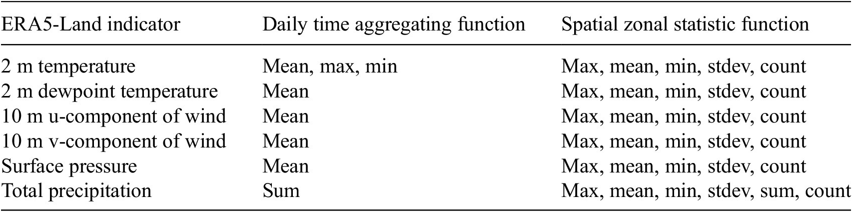
Abbreviations: Max, maximum; min, minimum; stdev, standard deviation; count, cells count.
The R script is available at GitHubFootnote 1 and the resulting NetCDF files are available at ZenodoFootnote 2.
2.3. Zonal statistics computation
As can be observed in Figure 1, the computation of zonal statistics considers the values from all cells that intersect the geographical boundary. For example, the mean zonal statistic can be expressed as:
 $$ \overline{X}=\frac{\sum \limits_1^n{x}_i}{n} $$
Where $ x $
is the value of the climate indicator on the cell
$ x $
is the value of the climate indicator on the cell $ i $
and
$ i $
and $ n $
is the total number of cells that intersect the spatial boundary. On this specification, the values of all cells that intersect the spatial boundaries are taken into account, disregarding the proportion of the cell that intersects the spatial boundary. Administrative boundaries may follow irregular patterns, leading to the inclusion of several cells on the zonal statistical computation that only slightly intersects the geographical boundary.
$ n $
is the total number of cells that intersect the spatial boundary. On this specification, the values of all cells that intersect the spatial boundaries are taken into account, disregarding the proportion of the cell that intersects the spatial boundary. Administrative boundaries may follow irregular patterns, leading to the inclusion of several cells on the zonal statistical computation that only slightly intersects the geographical boundary.
As suggested by Baston (Reference Baston2023), it is possible to weight the computation of the zonal statistics by considering the overlapping proportion of the cells over the spatial boundaries:
 $$ {\overline{X}}_c=\frac{\sum \limits_1^n{x}_i{c}_i}{\sum \limits_1^n{c}_i} $$
Where $ c $
is the proportional area of the cell
$ c $
is the proportional area of the cell $ i $
covered by the spatial boundary. This speciation results in a more realistic summarization of the climate indicator over a spatial boundary and was adopted in this work.
$ i $
covered by the spatial boundary. This speciation results in a more realistic summarization of the climate indicator over a spatial boundary and was adopted in this work.
To perform the computation of the zonal statistics on the daily aggregated indicators, an R package called zonalclim was developed. The package contains a function to create a list of tasks to be computed, splitting the layers available at the indicator files and the geographical boundaries into a number of chunks. This strategy was adopted to avoid overloading the random access memory by loading a potentially large number of climate data files and geographic boundaries at once. This list of tasks feeds a function that wraps the exactextractr package (Baston, Reference Baston2023) and performs the zonal statistics computation, writing its results in an SQLite database.
The Brazilian municipality boundaries from 2010 were used as a reference, provided by the “Instituto Brasileiro de Geografia e Estatística” (IBGE), the Brazilian official authority of administrative boundaries. The simplified boundaries version presented by the geobr (Pereira and Goncalves, Reference Pereira and Goncalves2022) package was used, which preserves the original topology with a tolerance of 100 m. The specific year of 2010 was adopted due to its compatibility with the population census conducted in the same year.
Table 1 summarizes the daily time aggregation functions and spatial zonal statistical functions applied to the climate indicators.
Thus, for each climate indicator, a number of spatial zonal statistical functions are applied to the daily time aggregation results. There are a total of eight daily climate indicators, leading to a total of 41 indicators computed for each day between 1950 and 2022.
The resulting daily climate indicators are converted to databases in the DuckDB (Mühleisen and Raasveldt, Reference Mühleisen and Raasveldt2023) format for faster columnar-vectorized queries and exported as parquet files (Richardson et al., Reference Richardson, Cook, Crane, Dunnington, François, Keane, Moldovan-Grünfeld and Ooms2023) for dissemination of results.
3. Results
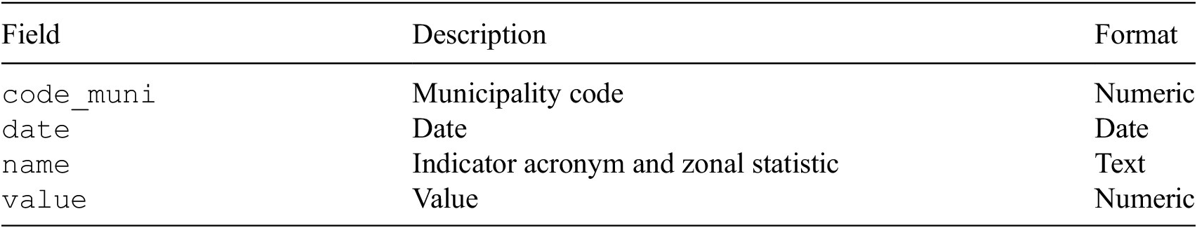
The available ERA5-Land data from 1950 to 2022 have been processed, and the computed zonal statistics are available to access at the parquet files listed in Table 2. These files follow a common schema, as presented in Table 3. As ERA5-Land data are updated monthly with a delay of three months, we plan to continuously update the zonal statistics dataset with new data at yearly intervals or more often if feasible.
Table 2. Parquet files, indicators, and units
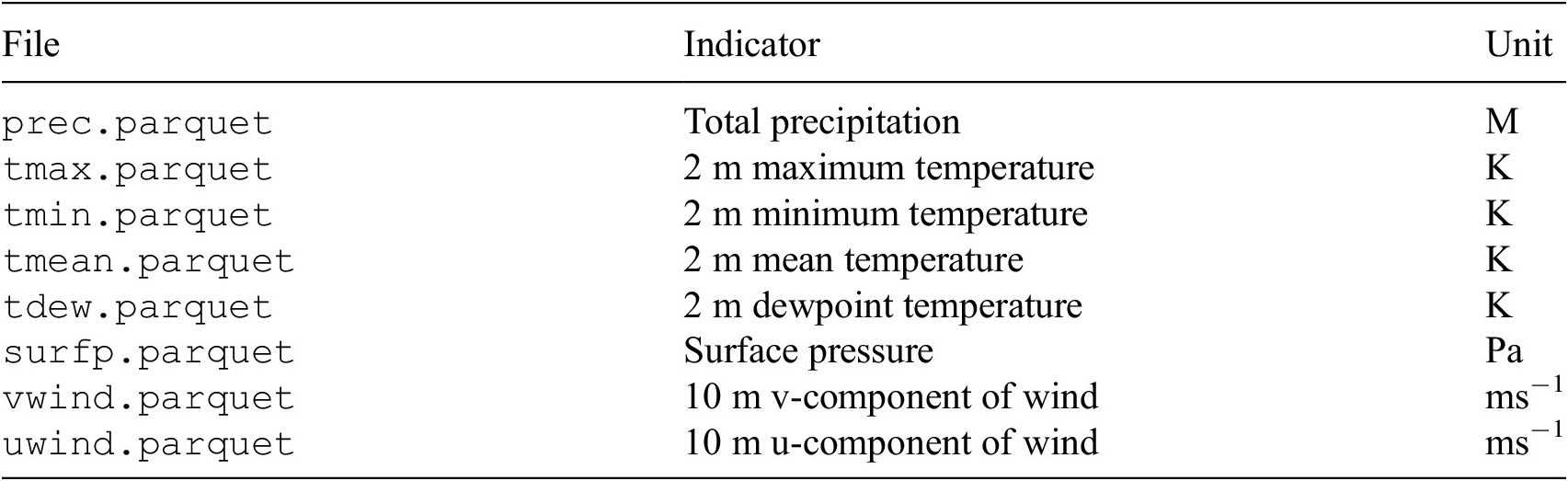
Table 3. Common parquet file schema
Together, those files present 6,085,749,761 records of daily climate indicators for Brazilian municipalities. The files are available for download at Zenodo: https://zenodo.org/doi/10.5281/zenodo.10036211.
Figure 2 presents a sample from the dataset, with the zonal statistic of average temperatures from the 27 Brazilian capitals. It is possible to observe at the figure different climate regimes, where municipalities like Belém, São Luiz, and Fortaleza present almost flat and stable temperatures over the months of all years. Differently, municipalities like Campo Grande, Curitiba, and Porto Alegre show lower temperatures over winter months (from June to September) on all years.
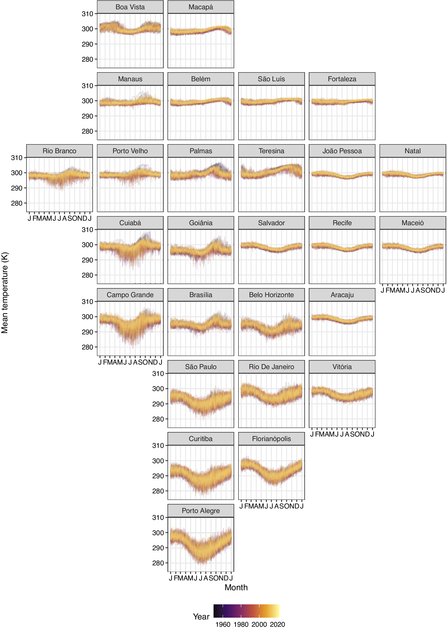
Figure 2.
Average daily temperatures ( $ K $
) from the 27 Brazilian capitals, from 1950 to 2022.
$ K $
) from the 27 Brazilian capitals, from 1950 to 2022.
Figures 3 and 4 are maps of the maximum and minimum zonal statistics of temperature ( $ k $
) for the Brazilian municipalities at January 1 on the years of 1950, 1960, 1970, 1980, 1990, 2000, 2010, and 2020. It is possible to observe at those maps how the maximum and minimum zonal statistics are spatially clustered over some groups of municipalities at this specific date, highlighting north and northeast parts of the country and also the municipalities at the south region of the country, localized in a mountain range.
$ k $
) for the Brazilian municipalities at January 1 on the years of 1950, 1960, 1970, 1980, 1990, 2000, 2010, and 2020. It is possible to observe at those maps how the maximum and minimum zonal statistics are spatially clustered over some groups of municipalities at this specific date, highlighting north and northeast parts of the country and also the municipalities at the south region of the country, localized in a mountain range.
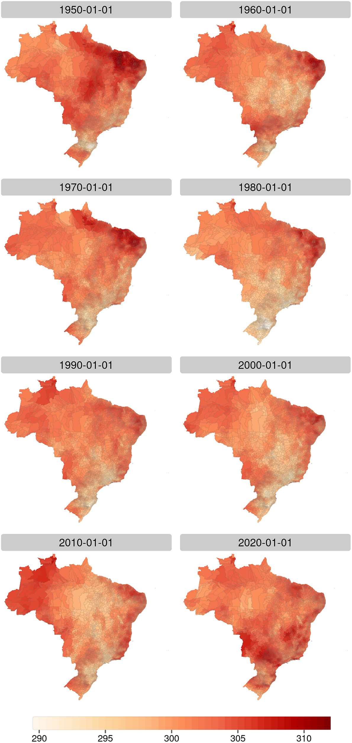
Figure 3.
Maximum zonal temperatures ( $ K $
) on Brazilian municipalities, for selected years.
$ K $
) on Brazilian municipalities, for selected years.
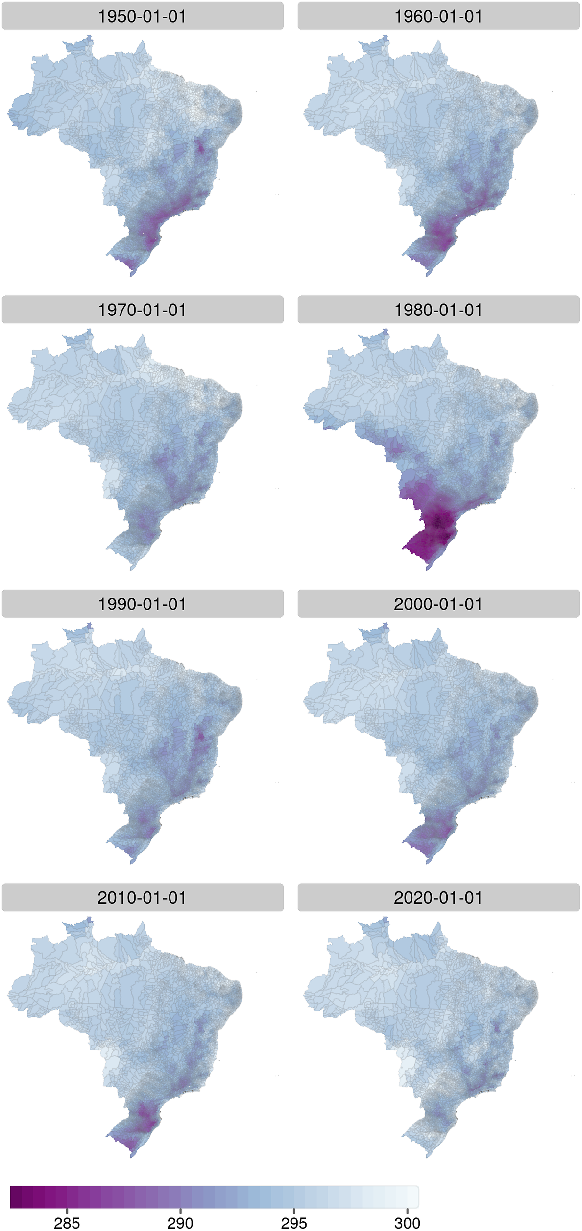
Figure 4.
Minimum zonal temperatures ( $ K $
) on Brazilian municipalities, for selected years.
$ K $
) on Brazilian municipalities, for selected years.
Figure 5 presents the sum and standard deviation zonal statistics of precipitation ( $ m $
) at the Rio de Janeiro municipalities on January 1, 2010. The standard deviation zonal statistic represents the spatial variability of the precipitation, where higher standard deviation values implies on precipitation concentrated on few grid cells, and the sum zonal statistic is the sum of the cell’s values. Considering those statistics together, it is possible to observe that the total precipitation was higher on two municipalities (Rio Claro on the center-west and Cachoeiras de Macacu on the east) but more concentrated in a different municipality (Angra dos Reis) on that specific date. The higher standard deviation of precipitation occurrence is directly related to a massive landslide occurred on that same day, which resulted in 50 deaths (de Mendonca and da Silva, Reference de Mendonca and da Silva2020; Memória Globo, 2021).
$ m $
) at the Rio de Janeiro municipalities on January 1, 2010. The standard deviation zonal statistic represents the spatial variability of the precipitation, where higher standard deviation values implies on precipitation concentrated on few grid cells, and the sum zonal statistic is the sum of the cell’s values. Considering those statistics together, it is possible to observe that the total precipitation was higher on two municipalities (Rio Claro on the center-west and Cachoeiras de Macacu on the east) but more concentrated in a different municipality (Angra dos Reis) on that specific date. The higher standard deviation of precipitation occurrence is directly related to a massive landslide occurred on that same day, which resulted in 50 deaths (de Mendonca and da Silva, Reference de Mendonca and da Silva2020; Memória Globo, 2021).
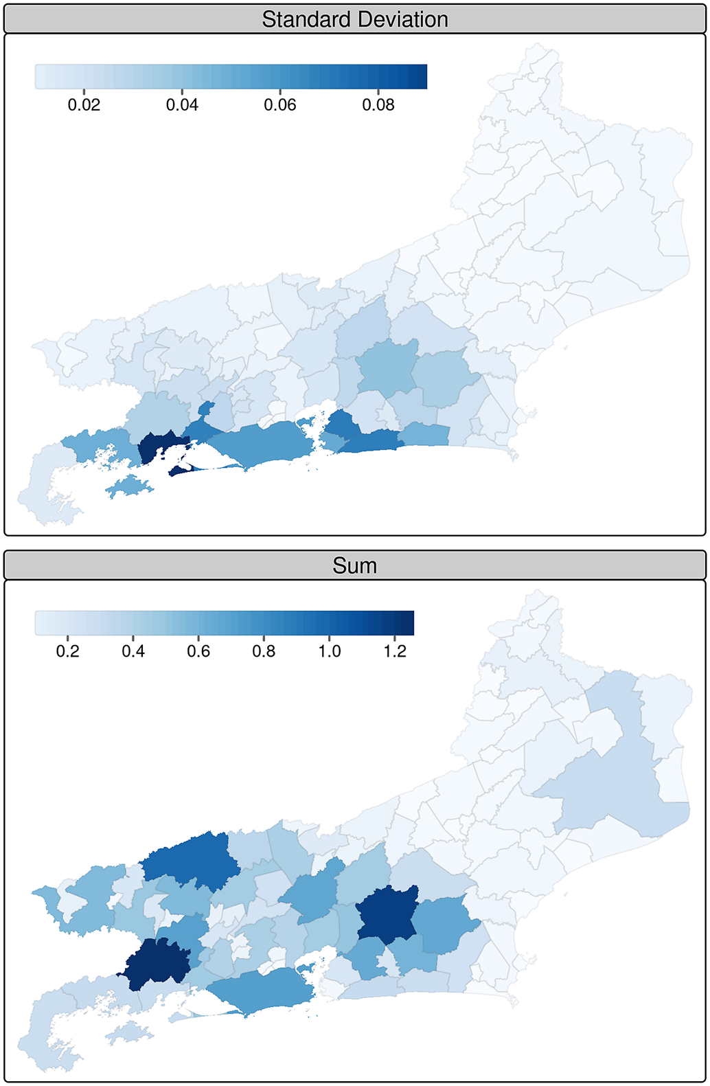
Figure 5.
Standard deviation and sum zonal statistics of precipitation ( $ m $
) at the Rio de Janeiro municipalities on January 1, 2010.
$ m $
) at the Rio de Janeiro municipalities on January 1, 2010.
Some of the zonal statistics—for example, mean, minimum, and maximum—may be re-aggregated in time by the user in order to create time series with monthly, quarterly, and other intervals.
Figure 6 presents the Köppen Climate Classification for the Brazilian municipalities, based on the proposed dataset, using data from 1990 to 2020. The daily zonal statistics of precipitation, maximum temperature, minimum temperature, and average temperature were aggregated to monthly periodicity using averages values, and the municipalities were classified with the ClimClass package (Eccel et al., Reference Eccel, Cordano and Toller2016). The obtained classes are well aligned with results from a study that adopted weather station data for the 1961–2015 period (Dubreuil et al., Reference Dubreuil, Pechutti Fante, Planchon and Neto2017).
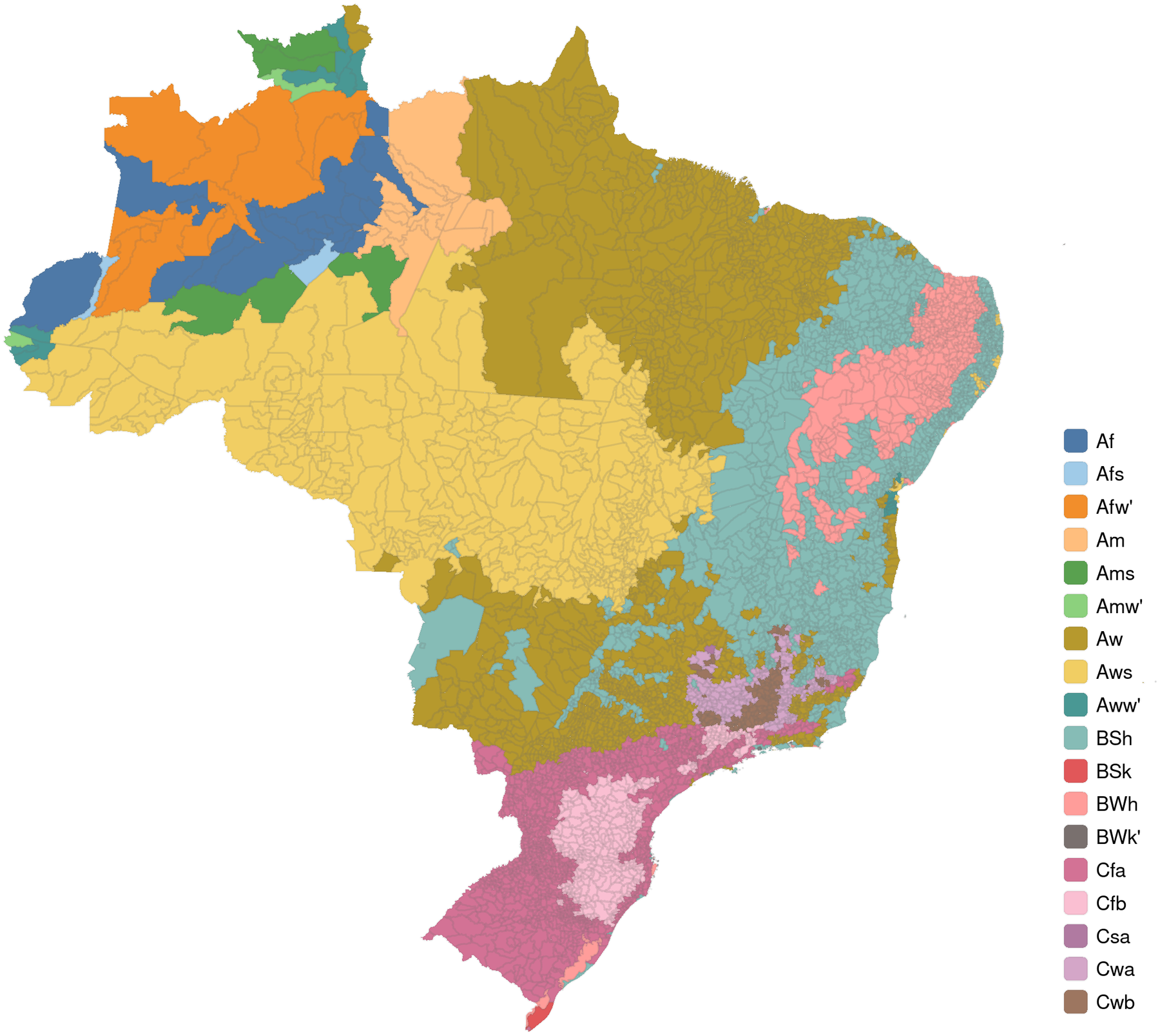
Figure 6. Köppen-Geiger climate classification of Brazilian municipalities, 1990 to 2020.
4. Discussion
The proposed methodology resulted in a dataset that will be useful for further researches that require climate indicators at the municipal scale of analysis. In comparison with published datasets of similar objective, our proposed dataset excels previous research by providing a longer time coverage of more than six decades at a finer daily time resolution. Also, our results present a rich set of six climate indicators that were spatially aggregated by zonal statistics with different strategies, which allows a more comprehensive representation of the spatial variability of the climate indicators over the municipalities’ territory.
The adopted methodology is fully reproducible, allowing the continuous update of the results as new data are made available by the ERA5-Land project and the inclusion of new climate indicators and other zonal statistics. The proposed methodology can be also easily extended to other territories of the globe to produce climate zonal statistics to other countries.
We believe that the proposed dataset will be helpful for climate-aware policymaking by presenting climate indicators spatially aggregated by municipalities, a fairly recognized and common boundary division for strategical planning in Brazil.
It is important to highlight that the interpretation and usage of zonal statistics to summarise the climate of administrative boundaries must consider the existing relationship between the boundaries area and the spatial resolution of the grid indicator. As with other statistical summary measures, the zonal statistics’ capacity to summarize values is directly related to the sample size and variance.
Figure 7 presents a histogram with the weighted area cell count in each municipality, with the $ x $
axis on logarithmic scale. The weighted area cell count represents the sum of entire cells and fractions used to compute the zonal statistics indicators in each municipality. The ERA5-Land grid is constant over the years for all indicators.
$ x $
axis on logarithmic scale. The weighted area cell count represents the sum of entire cells and fractions used to compute the zonal statistics indicators in each municipality. The ERA5-Land grid is constant over the years for all indicators.
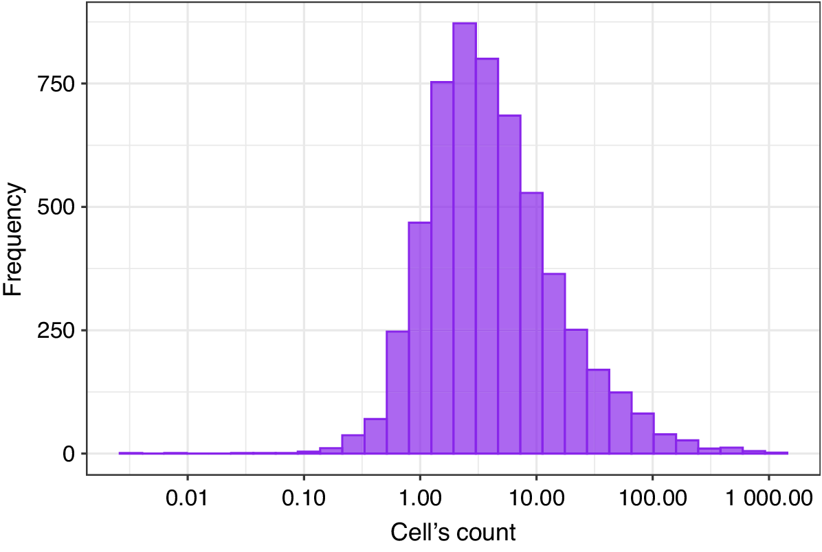
Figure 7. Histogram of weighted number of cells on a logarithmic scale.
There are 595 municipalities where the zonal statistics were computed using one cell or a fraction due to its small territorial area in comparison with the ERA5-Land cell size. The zonal statistics from 3,736 municipalities were computed with data from 1 to 10 cells, 1,138 municipalities with 10 to 100 cells, and 98 municipalities with more than 100 cells.
Municipalities with larger territorial areas will have more data points used for the zonal statistical computation. This may introduce a spatial variability in the zonal statistics, as the municipal area may cover a diversity of regions with different climate regimes. The spatial variability of the indicator may be observed by considering the standard deviation of the zonal statistic and the weighted cell count. Higher or lower values of standard deviations imply that there is, respectively, a larger or smaller variability in the values of the totality of cells used to compute the zonal statistic. Thus, the spatial variability measured by the standard deviation shows how concentrated or dispersed an indicator is in space, as illustrated by Figure 5.
5. Conclusion
In this work, we presented a consistent methodology to produce updated zonal statistics from gridded climate indicators for the Brazilian municipalities, resulting in the creation of a dataset of zonal statistics that covers a long time span at daily resolution and presents a full set of relevant climate indicators. The dataset access is facilitated by the adoption of the parquet file format for dissemination and may be updated periodically as new data are made available by the Copernicus program.
There are some possibilities that future research could address. To enhance the spatial resolution of the grid files, the application of statistical downscaling is possible by using interpolation or kriging methods (Chiles and Delfiner, Reference Chiles and Delfiner2012). For this, a list of suitable and available covariates for each climate indicator at higher spatial resolution must be compiled, and a study of the errors in the estimates is required.
Furthermore, the daily zonal statistics of climate indicators offered by this proposal may also be used to calculate weekly or monthly statistical time features of trends, persistence, and intensity. For example, indicators such as temperature variation ratio, number of consecutive days of rain, and number of days of an indicator below, above, or within some threshold may be computed by week or month interval. Also, some of the indicators proposed by the Expert Team on Climate Change Detection and Indices (ETCCDI) may be computed (World Meteorological Organization, 2009).
Punctual measures of weather indicators may also be extracted and presented as municipalities’ centroids or city hall localization, as adopted by the SISAM project. Considering the use of more refined spatial resolution grids, there is also the possibility of generating zonal statistics for different land covers and land use. The availability of zonal statistics for urban and rural areas, for example, may be useful for studies of urban vector diseases or for agriculture production.
These zonal statistics presented by this research may be used as a common source of data for different research projects, by presenting a standardized set of weather indicators for all municipalities for a long time span. The availability of direct access to weather indicators at the municipal level may speed up research in modeling lattice data, saving research time and effort.
Acknowledgments
This research was supported by Inria and LNCC.
Author contributions
R.S. data acquisition, data validation, writing, and project conception. V.R., C.C., E.P., and R.S. data validation and writing. R.A., M.P., P.V., and F.P. project conception. All authors reviewed the manuscript.
Data availability statement
The scripts created for the creation of the datasets are available at GitHub: https://github.com/rfsaldanha/brclim2. The ERA5-Land daily aggregates files are available at Zenodo: https://zenodo.org/communities/brclim. The resulting zonal statistics of climate indicators for Brazilian municipalities are available at Zenodo: https://zenodo.org/doi/10.5281/zenodo.10036211.
Funding statement
This research was supported by grants from Inria and CNPq Productivity Fellowship process number 312100/2021-3.
Competing interest
The authors declare no competing interests.
Ethics statement
The research meets all ethical guidelines, including adherence to the legal requirements of the study country.


 Open access