


Impact statement
We demonstrate the ability of deep learning models to successfully detect and classify fish in low-light deep underwater video data. We present video monitoring systems coupled with deep learning pipelines as a viable solution to safely monitor large marine ecosystems deep underwater that can be implemented at scale and at low costs to address the climate emergency. We show that 2,000 random images per species are sufficient to classify and detect a species of fish, and modern deep-learning models are capable of performing well in battery-operated light conditions. We expect these results to inform future data acquisition efforts. This work is the first step toward developing automated pipelines capable of continuously monitoring marine ecosystems deep underwater.
1. Introduction
Oceans and seas cover more than 70% of the planet (National Oceanic U.S. Department of Commerce and Atmospheric Administration, 2013). They create employment for 56 million people, host 80% of the planet’s biodiversity, regulate our climate, and are responsible for at least 50% of oxygen on Earth (UN Environment, n.d.). Despite their vital role in our climate, the sheer size and depth of the oceans mean they remain largely unobserved and not understood on a large scale because of the high costs and complexity involved in studying such a large ecosystem (Petsko, Reference Petsko2020). Precisely because of their vastness and complexity, they play an outsized role in regulating our climate (Bigg et al., Reference Bigg, Jickells, Liss and Osborn2003; Pörtner et al., Reference Pörtner, Roberts, Masson-Delmotte, Zhai, Tignor, Poloczanska and Weyer2019; UN Environment, 2016).
Many studies indicate that oceans act as a buffer against climate change (Roberts et al., Reference Roberts, O’Leary, McCauley, Cury, Duarte, Lubchenco, Pauly, Sáenz, Sumaila, Wilson, Worm and Castilla2017; Gattuso et al., Reference Gattuso, Williamson, Duarte and Magnan2021). Strategies to increase the alkalinity of the oceans and accelerate the weathering processes that naturally consume CO2 from the atmosphere (Renforth and Henderson, Reference Renforth and Henderson2017) or harvest tidal energy to generate greener alternative energy (Borthwick, Reference Borthwick2016; Melikoglu, Reference Melikoglu2018; Charlier, Reference Charlier1982) have been proposed as potential solutions to harness oceans to mitigate climate change. Despite careful efforts by researchers to assess the risks involved with adopting these solutions, the long-term consequences of these strategies on the ocean ecosystem are not very well understood (Bach et al., Reference Bach, Gill, Rickaby, Gore and Renforth2019). With aggressive targets needed to prevent the average global temperature from rising more than 2 °C in the next few decades (Rhodes, Reference Rhodes2016), we will need to adopt some or all of these strategies to be able to address this climate emergency before fully understanding the risks these strategies might pose (Cooley et al., Reference Cooley, Bello, Bodansky, Mansell, Merkl, Purvis, Ruffo, Taraska, Zivian and Leonard2019; Ordinary Things, Reference Bergman, Rinberg, Wilcox, Kolosz and Freemann.d.). It is thus critical that we develop affordable, scalable, and automated ocean monitoring solutions with low carbon footprints to closely monitor the effects of these solutions on the oceans and marine ecosystems.
Deep learning is a subset of machine learning that enables computer systems to learn from data by automatically extracting features that are representative of the data, and using these extracted features to make predictive decisions about new unseen data. Over the past decade machine learning has been successfully applied to data from varied domains like healthcare, robotics, entertainment, manufacturing, and transportation (Min et al., Reference Min, Lee and Yoon2017; Pierson and Gashler, Reference Pierson and Gashler2017; Da’u and Salim, Reference Da’u and Salim2020; Huang et al., Reference Huang, Chai and Cho2020; Gupta et al., Reference Gupta, Anpalagan, Guan and Khwaja2021; Yang et al., Reference Yang, Zhu, Ling, Liu and Zhao2021) to perform a diverse set of tasks ranging from detecting cancer in digital pathology images to recommending movies based on personal viewing history. One of the tasks deep learning models have proven to perform very well is object recognition. Object recognition combines object detection and classification to identify both the location and type of objects in an image. Object recognition models require a large number of image frames from videos annotated by experts and are then trained to detect objects from those different annotated classes in the images. Of the wide variety of object recognition models, there are two major families of object detectors, Region CNN (R-CNN) (Girshick et al., Reference Girshick, Donahue, Darrell and Malik2014; Sun et al., Reference Sun, Zhang, Jiang, Kong, Xu, Zhan, Tomizuka, Li, Yuan, Wang and Luo2021) and You Only Look Once (YOLO) (Bochkovskiy et al., Reference Bochkovskiy, Wang and Liao2020; Wang et al., Reference Wang, Bochkovskiy and Liao2022), that have demonstrated successful object recognition for a wide range of tasks and are continuously maintained and updated. The R-CNN family of models identifies different regions of interest in an image, extracts features from each identified region, and uses these extracted features to detect objects in an image; while the YOLO family of models divides the image into grids, extracts regions of interest in each of these grids, and detects objects from the extracted features from each of these grids. Kandimalla et al. (Reference Kandimalla, Richard, Smith, Quirion, Torgo and Whidden2022) compared Mask-RCNN and YOLO (version 3 and 4) models for detecting and classifying fish with DIDSON imaging sonar as well as cameras from fish passages and observed higher performance with the YOLO family of models. In this paper, we experiment with applying the YOLO family of models, specifically YOLOv4 (Bochkovskiy et al., Reference Bochkovskiy, Wang and Liao2020) and YOLOv7 (Wang et al., Reference Wang, Bochkovskiy and Liao2022), to detect and classify fish species deep underwater with dim battery-powered lighting.
Traditionally, ocean and marine ecosystems have been monitored using high-frequency radar, ocean gliders, and animal tagging (Bean et al., Reference Bean, Greenwood, Beckett, Biermann, Bignell, Brant, Copp, Devlin, Dye, Feist, Fernand, Foden, Hyder, Jenkins, van der Kooij, Kröger, Kupschus, Leech, Leonard, Lynam, Lyons, Maes, Nicolaus, Malcolm, McIlwaine, Merchant, Paltriguera, Pearce, Pitois, Stebbing, Townhill, Ware, Williams and Righton2017; Benoit Beauchamp and Duprey, Reference Benoit Beauchamp and Duprey2019; Lin and Yang, Reference Lin and Yang2020). These techniques are either invasive, human resource intensive, expensive, or do not scale to meet the climate emergency (Polagye et al., Reference Polagye, Joslin, Murphy, Cotter, Scott, Gibbs, Bassett and Stewart2020). Much research is underway to replace these traditional monitoring techniques with different forms of electronic monitoring using audio and video devices such as cameras, satellites, and acoustic devices (Lee et al., Reference Lee, Wu and Guo2010; Polagye et al., Reference Polagye, Joslin, Murphy, Cotter, Scott, Gibbs, Bassett and Stewart2020; Hussain et al., Reference Hussain, Wang, Ali and Riaz2021; Kandimalla et al., Reference Kandimalla, Richard, Smith, Quirion, Torgo and Whidden2022; Rizwan Khokher et al., Reference Rizwan Khokher, Richard Little, Tuck, Smith, Qiao, Devine, O’Neill, Pogonoski, Arangio and Wang2022; Zhang et al., Reference Zhang, O’Conner, Simpson, Cao, Little and Wu2022). As such, several researchers have applied deep learning to specifically classify and detect different species of marine life for various applications (Qin et al., Reference Qin, Li, Liang, Peng and Zhang2016; Salman et al., Reference Salman, Jalal, Shafait, Mian, Shortis, Seager and Harvey2016; Sun et al., Reference Sun, Shi, Liu, Dong, Plant, Wang and Zhou2018). Collecting and annotating underwater video is time consuming and expensive so most testing of deep learning models to classify fish species uses publicly available fish datasets like the Fish 4 Knowledge dataset (Boom et al., Reference Boom, He, Palazzo, Huang, Beyan, Chou, Lin, Spampinato and Fisher2014) and LifeCLEF datasets (Ionescu et al., Reference Ionescu, Müller, Villegas, de Herrera, Eickhoff, Andrearczyk, Cid, Liauchuk, Kovalev and Hasan2018). Siddiqui et al. (Reference Siddiqui, Salman, Malik, Shafait, Mian, Shortis and Harvey2018) used deep learning to classify 16 species of fish from data captured using two high-definition video cameras over 60 min along a depth of 5–50 m; Cao et al. (Reference Cao, Zhao, Liu and Sun2020) used deep learning to detect and estimate the biomass of live crabs in ponds. More recently, Simegnew Yihunie Alaba et al. (Reference Simegnew Yihunie Alaba, Shah, Prior, Campbell, Wallace, Ball and Moorhead2022) used deep learning to detect species of fish in the large-scale reef fish SEAMAPD21 (Boulais et al., Reference Boulais, Alaba, Ball, Campbell, Iftekhar, Moorehead, Primrose, Prior, Wallace, Yu and Zheng2021) dataset collected from the Gulf of Mexico continental shelf at water depth, ranging from 15 to 200 m.
In general, image-based machine learning research for life underwater has been limited to deploying cameras on fishing vessels, shallow waters, aquariums, or aquaculture establishments, with only limited work extending these camera monitoring systems to deep underwater because of the challenges involved in acquiring and analyzing underwater video data below the sunlight zone. To the best of our knowledge, machine learning applications for fish species detection deep underwater have not been explored. This may be because of the challenges involved including data collection and annotation, low-resolution camera images, low light, multiple fish in the same frame, occlusion of fish behind rocks on the ocean floor, and blurring caused by fish movement, all of which make the application of deep learning on such data challenging.
We explored the application of deep learning object recognition models to a dataset containing multiple species of fish collected by the Canadian Department of Fisheries and Oceans by placing arrays of hundreds of inexpensive underwater cameras along with a battery-operated light source and bait deep underwater off the coast of Newfoundland, Canada. We aimed to detect and classify multiple different species of fish in underwater video data from a marine protected area with the goal of studying the impact of nearby human activity such as seismic testing on fish in a protected area. However, placing cameras to monitor these marine ecosystems may be intrusive to marine life. Research has shown that marine ecosystems are influenced by human activity, light, and sound (Davies et al., Reference Davies, Coleman, Griffith and Jenkins2015). To minimize the adverse effects large-scale data monitoring may cause to marine life, we were particularly interested in learning best practices to acquire this data such as how much data, what type of data, and how much light is required to train a useful machine learning model. To that end, we conducted experiments to determine the number of samples of different species of fish required to develop an efficient and accurate deep-learning model and observed the performance of the trained models on videos acquired in low light conditions as the battery-operated lights waned.
In this paper, we present the results from successfully training YOLOv4 and YOLOv7 models to classify and detect six species of fish with a mean average precision value(mAP) value of 76.01% and 85.0%, respectively. We argue that 2,000 sampled images of each class of fish are sufficient to train a model successfully, and show that the trained models perform efficiently in low-light conditions. As deep learning models are ever improving, we also compare and contrast the performance of the YOLOv4 and YOLOv7 models and analyze the limitations in the performance of each of the trained models. Additionally, we identify the challenges involved with detecting and classifying the rarer species in this dataset and propose strategies to address the challenges involved with this and future datasets. Finally, we identify the challenges and opportunities that must be solved to scale a system that could continuously monitor marine ecosystems worldwide to meaningfully tackle climate action.
2. Material and Methods
2.1. Machine learning models
YOLO family of models are deep learning architectures that classify and detect objects of different classes in an image. They have been successfully applied to detect objects from different domains (Nugraha et al., Reference Nugraha, Su and Fahmizal2017; Laroca et al., Reference Laroca, Severo, Zanlorensi, Oliveira, Gonçalves, Schwartz and Menotti2018; Seo et al., Reference Seo, Sa, Choi, Chung, Park and Kim2019). These models read an image; divide the image into n by n grid cells; identify regions of interest in each of the grid cells and assign confidence values for each identified region of interest. Each grid cell is also assigned a class probability map which quantifies the uncertainty with which the model detects an object of a particular class in that grid cell. The identified regions of interest are then aggregated and assigned confidence values to detect objects of different classes in the image.
2.1.1. YOLOv4
The YOLOv4 architecture has three major components: the backbone, the neck, and the head (Bochkovskiy et al., Reference Bochkovskiy, Wang and Liao2020). The backbone of this architecture is designed to extract features in the data and feed the extracted features to the head through the neck. The backbone uses a 53-layer convolutional neural network called CSPDarknet53 that extracts features from objects of three different scales in an image. The neck of this model collects feature maps from different stages of the feature extractor using a Spatial Pyramid Pooling (SPP) addition module and combines them with a Path Aggregation Network (PAN). The head of this network predicts confidence values for more than 20,000 possible bounding boxes of various sizes from these feature maps. These bounding boxes are then aggregated using a non-max suppression algorithm to detect non-overlapping objects in the image.
2.1.2. YOLOv7
YOLOv7 (Wang et al., Reference Wang, Bochkovskiy and Liao2022) improves on YOLOv4 by using modern strategies to train more efficiently and deliver better object detection performance. Note that, despite the name, YOLOv7 is the next model from the developers of YOLOv4 and the model name YOLO has a complicated history (Tausif Diwan and Tembhurne, Reference Tausif Diwan and Tembhurne2022). In comparison with YOLOv4, YOLOv7 reduces the number of parameters by 75%, requires 36% less computation, and achieves 1.5% higher AP (average precision) on MS COCO dataset. YOLOv7 uses several optimizations that are claimed to contribute to improved speed without compromising accuracy. Some of them are a better computational block called E-ELAN, a modified version of Efficient Long-Range Attention Network for Image Super-resolution(ELAN) (Zhang et al., Reference Zhang, Zeng, Guo and Zhang2022) in its backbone that enables YOLOv7 to optimize its learning ability; compound model scaling to maintain the properties that the model had at the initial design and maintain the optimal structure to efficiently use all the hardware resources while scaling model to suit different application requirements; an efficient module level re-parameterization that uses gradient flow propagation paths to choose the modules that should use re-parameterization strategies to train a model that is more robust to general patterns that it is trying to learn; an auxiliary head in the middle layers of the network with coarse-to-fine grained supervision from the lead head at different granularities to improve the performance of the model.
2.2. Evaluation metrics
Object classification and detection models are evaluated by the following performance metrics:
-
• Classification confidence: The detected object is classified into one of the classes the model has been trained on. A corresponding confidence value is assigned to signify the level of uncertainty with this class assignment. This enables filtering low-confidence objects for applications such as fish detection to improve precision.
-
• Intersection over Union (IoU): IoU measures how accurately the model’s detection matches with the manually labeled ground truth. IoU of 0 implies that no part of the predicted detection overlaps with the ground truth bounding box, while an IoU of 1 implies that the predicted detection perfectly matches the ground truth bounding box. It is computed as the ratio of the area of overlap and area of union between the ground truth and predicted bounding boxes (Figure 1).
-
• Precision: Precision measures the fraction of fish detections that are actually correct. A model that has a precision of 1.0 identifies all fish objects and does not detect any non-fish objects.
 $$ \mathrm{Precision}=\frac{\mathrm{True}\ \mathrm{Positives}}{\mathrm{True}\ \mathrm{Positives}+\mathrm{False}\ \mathrm{Positives}} $$
-
• Recall: Recall measures the fraction of fish objects correctly detected by the model. Recall is 1.0, if all the fish objects were correctly detected as fish, and the recall is 0.0, when a model fails to detect any fish object.
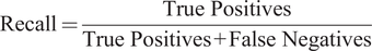 $$ \mathrm{Recall}=\frac{\mathrm{True}\ \mathrm{Positives}}{\mathrm{True}\ \mathrm{Positives}+\mathrm{False}\ \mathrm{Negatives}} $$
-
• Mean Average Precision (mAP): mAP is the mean of average precision (AP) across all the classes in the dataset. AP is computed as the weighted average of the average precision over various IoU thresholds with the weight being the difference in recall from the previous IoU threshold. mAP is designed to balance both the precision and the recall values taking into account both the false positives and false negatives to determine the performance of a detector. This is the standard measure used to compare the performance of object classification and detection models. We use this measure to determine how many samples of each class are required to train an efficient machine-learning model.
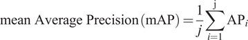 $$ \mathrm{mean}\ \mathrm{Average}\ \mathrm{Precision}\;\left(\mathrm{mAP}\right)=\frac{1}{j}\sum \limits_{i=1}^{\mathrm{j}}{\mathrm{AP}}_i $$
with $ {AP}_i $
being the average precision of the ith class and j being the total number of classes.
$ {AP}_i $
being the average precision of the ith class and j being the total number of classes.
 $$ \mathrm{Average}\ \mathrm{Precision}\left(\mathrm{AP}\right)=\sum \limits_{k=0}^{n-1}\left[\left(\mathrm{recall}\left(\mathrm{k}\right)-\mathrm{recall}\left(\mathrm{k}+1\right)\right)\times \mathrm{precision}\left(\mathrm{k}\right)\right], $$
where $ n $
is the number of ground truth objects and k is an index representing each object in the ground truth, ranging from 0 to n − 1.
$ n $
is the number of ground truth objects and k is an index representing each object in the ground truth, ranging from 0 to n − 1.
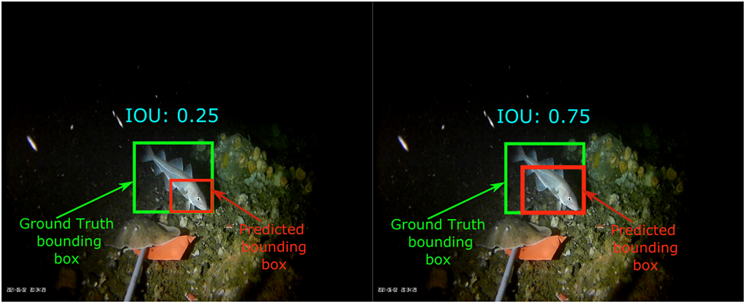
Figure 1. Intersection over union.
2.3. Data
Inexpensive cameras with bait to attract fish were placed and later recovered from an approximate depth of 450–500 m along the marine slopes of the Northeast Newfoundland marine refuge to determine the impact of nearby seismic testing on fish in the marine protected area (Barnes et al., Reference Barnes, Schornagel, Whidden, Morris and Lamontagnen.d.). There is very little light past 200 m (National Oceanic U.S. Department of Commerce and Atmospheric Administration, n.d.) in the ocean so a light source powered with a 6 V battery was placed along with each camera to acquire this dataset. These batteries deplete over time resulting in low and varying brightness in the captured videos. The brightness of a video is computed by averaging the pixel values in the “value” channel of all the frames in HSV color space. As can be observed in Figure 2a, 90% of videos in the dataset have an average brightness less than 17. For reference, a fully white video would have a brightness of 255. We also note that as the day progresses, the battery starts depleting, resulting in decreasing average brightness (Figure 2b).
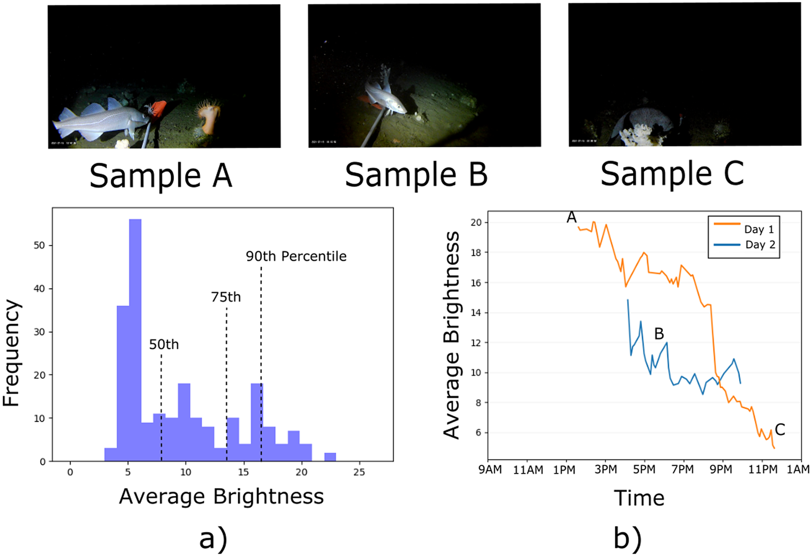
Figure 2. (a) Variation of brightness in the dataset. (b) Variation of average brightness over time. Brightness is measured by the average “Value” channel in HSV color space across frames of each video.
We acquired 221 videos in total over a 3-day deployment across an approximately one km radius in the northeast Newfoundland slope Marine Refuge in the Atlantic Ocean. Video was captured at 30 frames per second and in 5-minute long sequences. We extracted 1502 frames from each video using Python’s OpenCV library. The captured videos were annotated by a fish expert at DFO, using the VIAME platform (VIAME Contributors, 2017). The YOLO family of models requires a text file for each image frame with annotations for all the objects in that frame. Each text file has the same name as the image frame and must be in the same directory. Each line in the text file corresponds to a distinct object in the frame that represents an object with a bounding box which constitutes four values: [x_center, y_center, width, height]. YOLO normalizes the image space to run from 0 to 1 in both the x and y directions. As such, the manually annotated bounding boxes are normalized with respect to the image dimensions to represent values in the normalized image space. Text files with the name of the frames in the expected YOLO format are created for all the frames in train, validation, and test splits. For frames without any objects, an empty text file is created.
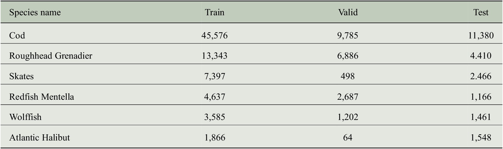
The annotated dataset has 10 distinct species of fish, with the distribution set shown in Table 1. Owing to the shared feature set between the subspecies of certain species and the lack of enough distinct examples for each of the subspecies, we have combined examples from the subspecies “Thorny Skates” and “Spinytail Skates” into a single class “Skates” and the examples from the subspecies “Striped Wolffish” with the class “Wolffish”. The species “Whelk” and the species labeled as “Unknown” have a single unique example of each of the species in a video respectively which is not sufficient data to train a detection and classification model. As such, these 2 videos were removed from the dataset. After this preprocessing, we trained our models on 219 videos with 6 distinct classes. The 219 videos were randomly assigned to train, validation and test splits in a roughly 70–15-15 ratio based on the frequency of frames with fish in each video. Analysis of the class distribution in each of these splits revealed that all the videos for the species Atlantic Halibut were allocated to the train split. To balance the presence of this species in all three splits, videos from this class were randomly reassigned with an approximately 70–15-15 ratio. To avoid data leakage between our splits any frames from the same video must be in the same split. The final distribution of species in train, validation, and test splits are shown in Table 2.
Table 1. Number of unique objects in each class (Sample frequency) and number of videos with annotated objects from each class (video frequency) in the manually annotated label set.
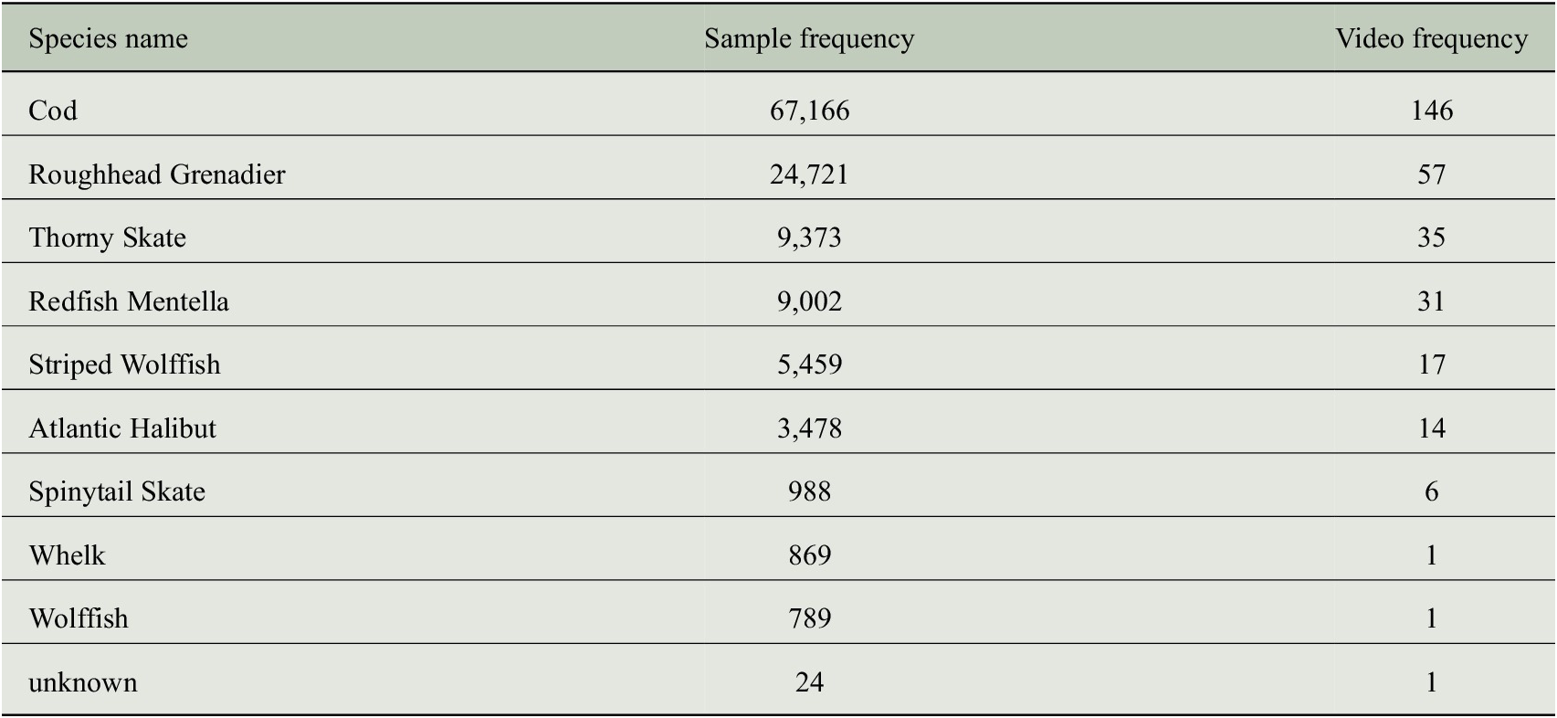
Table 2. Number of objects of each species of fish in train, valid, and test splits.
2.4. Experiment setup
To start training, frames with annotated fish in their frames, for all the videos in the split are listed in a text file for each split. The models are trained on the frames in the training split and the frames in the validation split are used during training for hyperparameter tuning. Although the validation set is used by the models during training, it is important to note that the model never trains on the frames in the validation set. To set up the baseline, a YOLOv4 (Bochkovskiy et al., Reference Bochkovskiy, Wang and Liao2020), and a YOLOv7 (Wang et al., Reference Wang, Bochkovskiy and Liao2022) model are trained to classify and detect the 6 classes of fish in the entire dataset.
In order to quantify the number of samples of each class required, subsamples of 200, 500, 1,000, and 2,000 are randomly subsampled from each class in the training set. Models are trained on each of these subsampled sets and evaluated on the validation set to quantify the number of samples from each class required and determine the IoU threshold required for this dataset to train an efficient machine learning model, which are treated as hyperparameters in our experimental setup. These hyperparameters are used to evaluate the detections on the test set.
2.5. Model training
2.5.1. Training the YOLOv4 model
Machine learning models use a lot of hyperparameters that heavily influence the training process and the performance of the trained models. These hyperparameters depend on various factors like the architecture of the model, size of the dataset and the size of the GPU used for training. The authors of Darknet, along with the source code, published a set of guidelines to optimally set hyperparameters and successfully train a machine learning model on a custom dataset. We follow their recommendations where applicable and use the default values listed in the YOLOv4.config for the rest of the hyperparameters, including the augmentation parameters. The following paragraph lists the parameters that have been modified, following the issued guidelines.
Hyperparameters batch and subdivisions are set to 32 and 16 respectively to fit the batch into the GPU the models are trained on. Sixteen sets of 32 images are randomly sampled by the model from the training set and the gradient for the batch is computed on each set of 16 images over 32 batches. The parameters width and height are both set to 640 to match the recommended image size of YOLOv7 model. The YOLOv4 model resizes the input image to size 640 × 640 and scales the ground truth bounding boxes accordingly before starting to train on the images. It is recommended that a minimum of 2,000 unique examples from each class be seen for efficient detection and classification for this architecture. The parameter max_batches, which decides the number of iterations the model trains on was set to number of training images if the number of training images is less than (number of classes * 2,000); otherwise, the parameter is set to the total number of training images, following the recommendation by the YOLOv4 developers. The parameter classes is set to 6 since we have 6 classes in our dataset. The parameter filter which denotes the number of output parameters, computed as (classes + 5) * 3 was set to 33.
We started training our models with the pre-trained weights of the convolution layers from a YOLOv4 model trained on Microsoft Common Objects in Context (MSCOCO) dataset (Lin et al., Reference Lin, Maire, Belongie, Bourdev, Girshick, Hays, Perona, Ramanan, Zitnick and Dollár2014). The MSCOCO dataset is a large-scale image dataset of real-world objects and classes with over 200,000 labeled images and 80 classes. Pre-training our model allows us to retain the semantically rich information the model has gained while learning to detect and classify the 80 classes in the MSCOCO dataset and transfer that knowledge to the task of detecting and classifying fish in our dataset, and is a common practice in training deep learning models.
The models are trained on NVIDIA A100 GPU for the number of iterations specified by the max_batches parameter. We stop training after max_batches number of iterations. The models overfit before we stop the training. The models with the lowest validation loss for evaluation purposes.
2.5.2. Training the YOLOv7 model
The source code of YOLOv7, implemented in Python and published by the authors on GitHub is cloned to train models with this architecture. Similar to YOLOv4, the models are pre-trained with YOLOv7 models trained on MSCOCO dataset. A batch_size of 32 and Image dimensions of 640 × 640 are used to train these models. The models are trained on a single GPU node with eight CPU workers for 200 epochs, and the model with the lowest validation loss is used for evaluation purposes.
The configuration file present in cfg/training/YOLOv7.yaml is used for training. The parameter nc is changed to 6 since we have six classes in our training set. No modifications are made to the number of anchors or the architecture of the model. The default hyperparameters present in data/hyp.scratch.p5.yaml were used with no modifications.
3. Results
3.1. Deciding hyperparameters: IoU threshold and number of training samples
The trained models were validated on all the frames with fish from the videos in the validation set. As a reminder, the validation set has no overlap with the training set and is used to tune the performance of models and select hyperparameters. The mAP of the models was calculated across a range of IoU thresholds to study the detection quality of the trained models. At higher IoU thresholds the predicted bounding box must closely match the manual ground truth annotation to be considered a detection, with the predicted bounding box required to coincide exactly with manual ground truth annotation at an IoU threshold of 1. As such, we expect mAP to decrease as the IoU threshold increases toward 1. Deep learning models typically perform better with a large amount of data, so we expect our models trained with a larger number of training frames to achieve higher mAP at a given IoU threshold.
Figures 3 and 4 demonstrate the performance of the models trained using both YOLOv4 and YOLOv7 architectures, respectively. As expected, we observe that the models trained with all the frames in the training set perform the best in both experiments and the mAP decreases at higher thresholds in both architectures. Surprisingly, YOLOv4 models achieved higher mAP values than YOLOv7 at low thresholds but the performance of YOLOv4 started to drop at a threshold of 0.4 and drops rapidly when IoU thresholds exceed 0.5. In contrast, YOLOv7 models maintain a high mAP for IoU thresholds up to 0.9. This implies that although YOLOv7 models miss more detections than YOLOv4 models, the detections are more closely aligned with the manually annotated ground truth boxes. We also observed that models trained with 1,000–2,000 samples achieved similar mAP compared to the baseline models trained with all the training frames in the dataset.
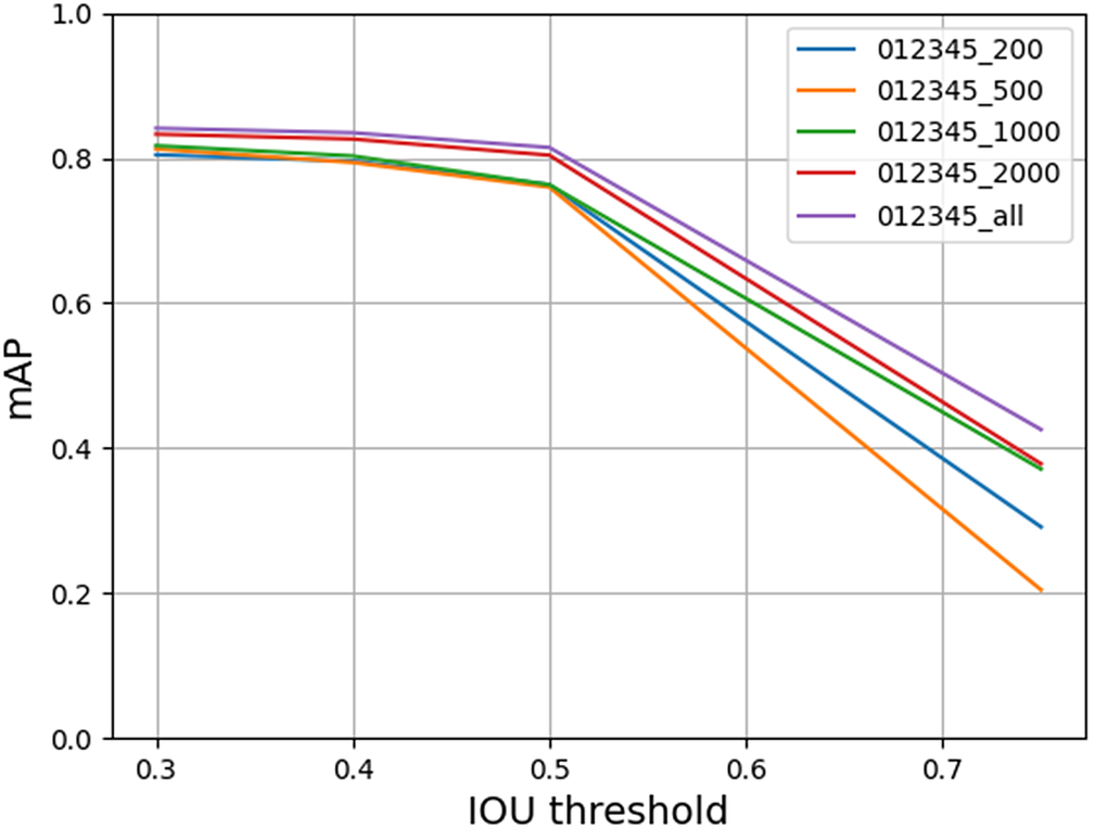
Figure 3. mAP at different IoU thresholds for models trained with 200, 500, 1,000, 2,000, and all samples of fish in each class using YOLOv4 architecture.
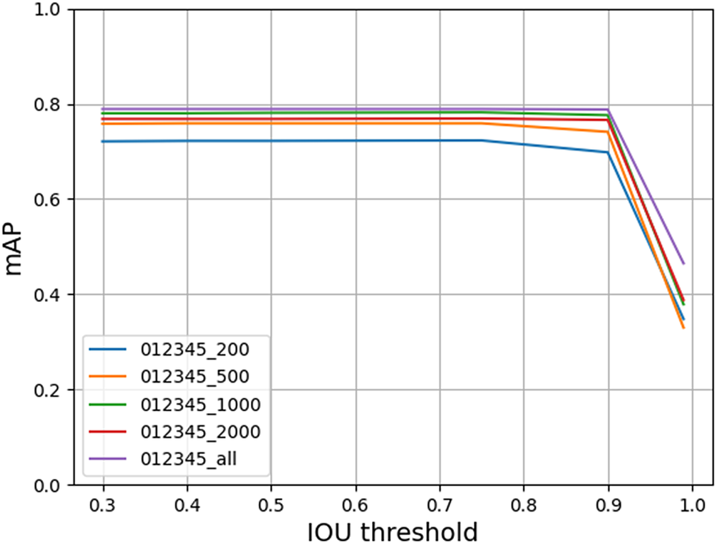
Figure 4. mAP at different IoU thresholds for models trained with 200, 500, 1,000, 2,000, and all samples of fish in each class using YOLOv7 architecture.
Based on these results, we consider 2,000 frames of each class with an IoU threshold of 0.4 as the ideal hyperparameters from this evaluation of the trained models on the validation set. The YOLOv4 and YOLOv7 models trained with 2,000 frames of each class were then evaluated at the IoU thresholds of 0.4 and 0.6 to compare the performance of both the trained models on the test set.
3.2. Evaluation on test set
We evaluated our YOLOv4 and YOLOv7 models trained on 2,000 samples of each class at IoU thresholds of 0.4 and 0.6 on the frames with fish in all the videos of the test set. As a reminder, the test set has no overlap with the training or validation sets and no models were evaluated on the test set until we completed the model training and experiments above and began writing this paper. The YOLOv4 model achieved an mAP of 89.32% at an IoU threshold of 0.4 and an mAP of 76.01% at the IoU threshold 0.6, while the YOLOv7 model achieved an mAP of 85.0% at both the IoU thresholds of 0.4 and 0.6.
Figure 5 compares the mAP of the models trained with YOLOv4 and YOLOv7 at thresholds 0.4 and 0.6 across the different species in the dataset and Figures 6 and 7 show the confusion matrices for the models trained with YOLOv4 and YOLOv7 and evaluated at an IoU threshold of 0.4. The YOLOv7 model detected more false positives in most classes, with the exception of Skates, while YOLOv4 detected more false negatives. In other words, YOLOv4 makes fewer mistakes in the objects it detects as fish but misses a relatively larger number of fish; whereas YOLOv7 detects more fish correctly but also makes more mistaken identifications. We observed that both trained models made more mistakes attempting to detect species trained with frames from fewer videos. For example, both models missed many Wolffish (68% detected with YOLOv4, 74% detected with YOLOv7) and Atlantic Halibut (81% YOLOv4 and 87% YOLOv7). The entire dataset only has 18 videos of Wolffish and 14 videos of Atlantic Halibut. Since the frames used to train the models must be subsampled from fewer videos, the data used by the models to detect and classify these species have less variation compared to the data used to train other species. We observe that 2,000 frames is a good baseline requirement for each species of interest. Both YOLOv4 and YOLOv7 can be trained on underwater video data to detect and classify different species of fish with as little as 2,000 frames, with the caveat that the data used to train the models must be representative of the test set if the models are expected to learn a general representation of the objects from a particular class.
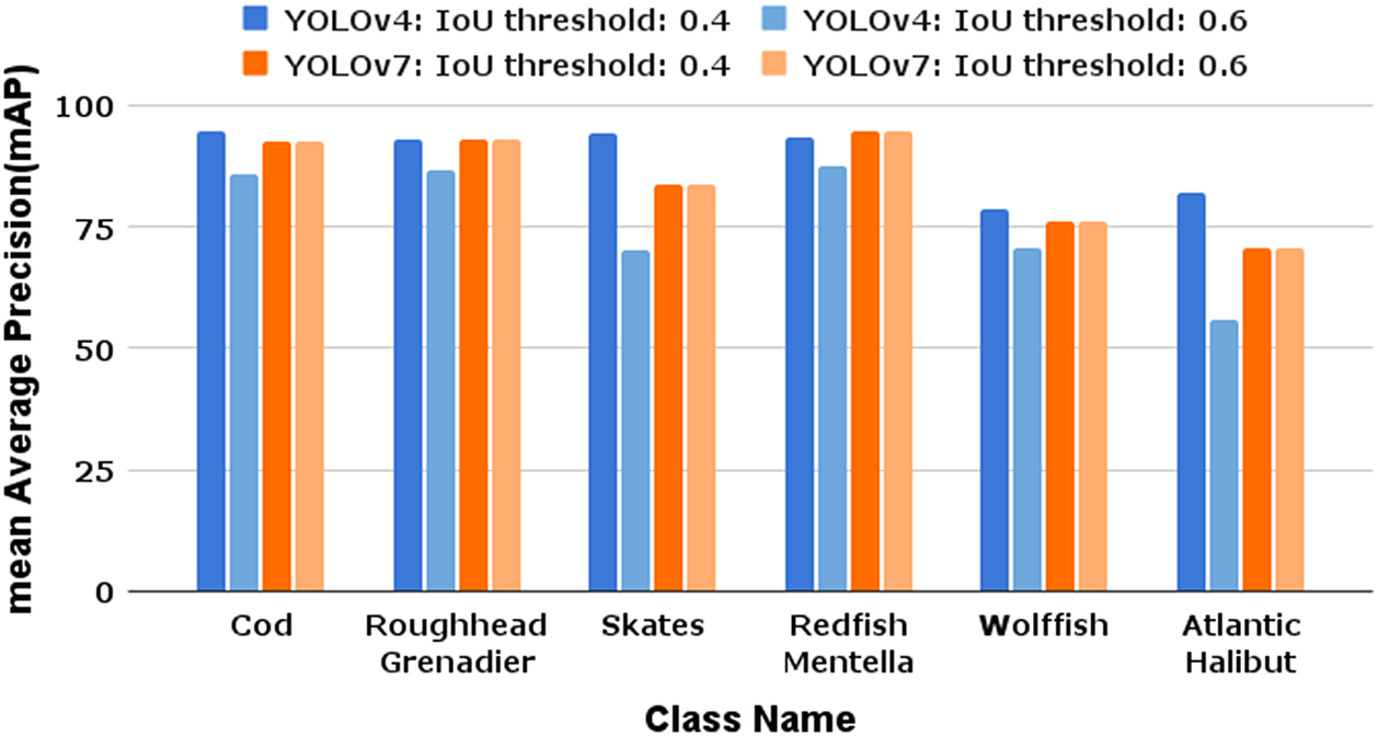
Figure 5. mAP of the models trained with 2,000 species in each class for both YOLOv4 and YOLOv7 models evaluated at thresholds of 0.4 and 0.6.
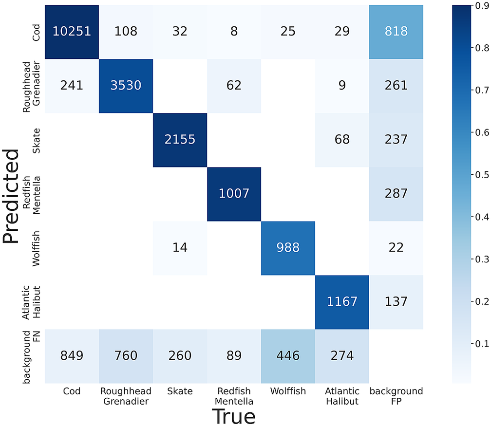
Figure 6. Confusion matrix for the YOLOv4 model trained with 2,000 samples in each class evaluated at IoU threshold of 0.4.

Figure 7. Confusion matrix for the YOLOv7 model trained with 2,000 samples in each class evaluated at IoU threshold of 0.4.
3.3. Evaluation on water frames
So far, we have presented the results of our models trained and evaluated only on frames known to contain fish. However, if such a model is to be deployed on camera data then the trained models must perform well on full videos which, in our dataset, contain an average of 60–70% frames that do not contain any fish. For clarity, we refer to frames with just water and no annotated fish objects as water frames. Our test set has 37 videos, with 55,574 frames, out of which 36,327 frames have no annotated fish in them, that is, 65.41% of all frames in the test set are water frames. We next evaluated our YOLOv4 and YOLOv7 models, trained with 2,000 samples of each class, at IoU threshold of 0.4 and 0.6 on just the water frames in the test set to probe the performance of these trained models on full videos. The YOLOv4 model falsely detects a fish object in 10.3% and 8.4% of the water frames at IoU thresholds 0.4 and 0.6, respectively, while the YOLOv7 model falsely detects a fish object in 12.5% of the water frames at both the IoU thresholds. YOLOv4 model falsely detects fish objects in a lesser percentage of water frames. This correlates with our observations thus far that YOLOv4 detects fewer fish objects at higher thresholds. However, examining some of these misclassifications revealed that many of our purported false positives are actually true positives that were missed during manual annotation due to human error. See Figure 8 for examples of fish detected by the YOLOv7 model that were not annotated in our dataset during manual annotation.
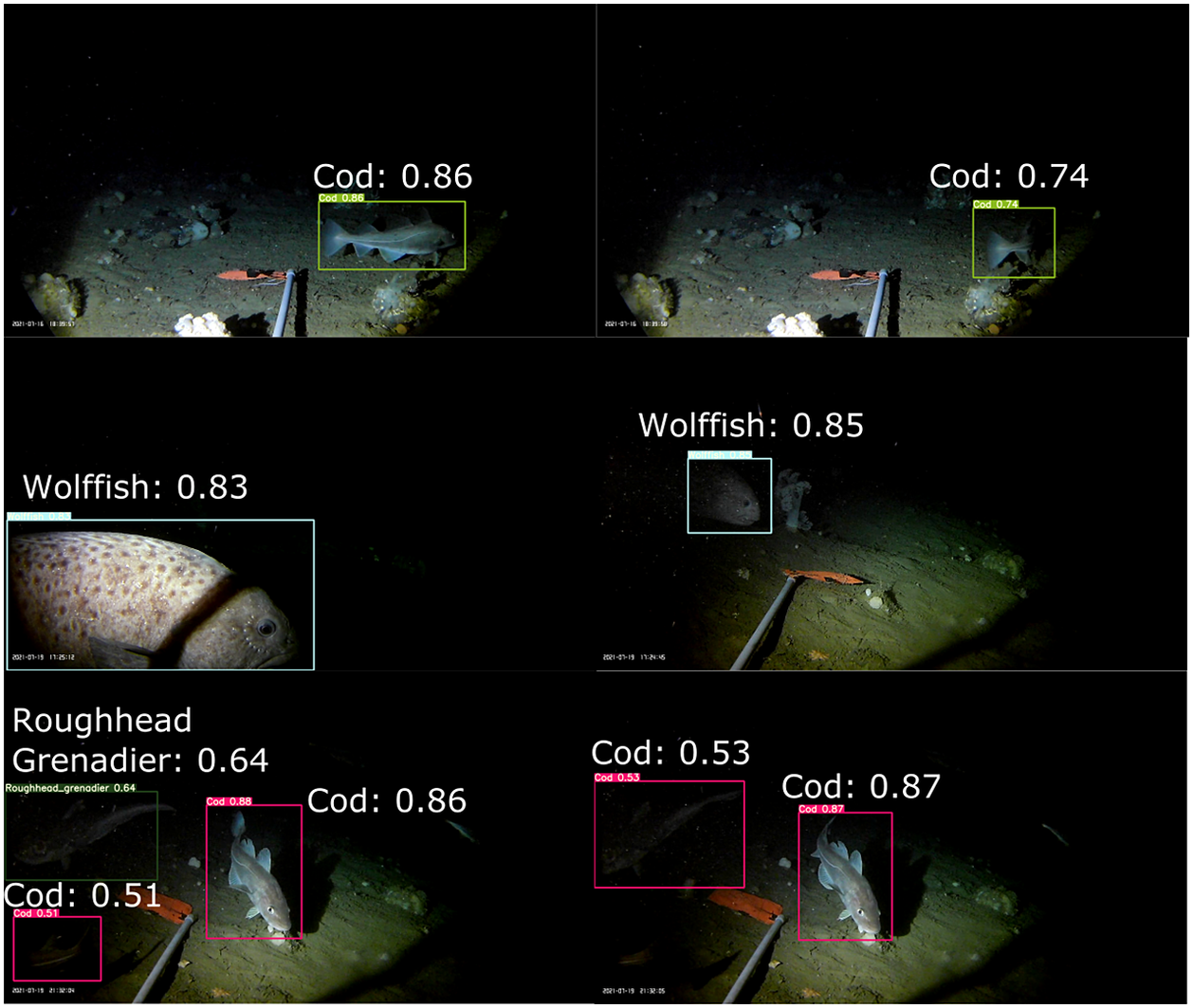
Figure 8. Examples of fish objects identified in water frames by the YOLOv7 model trained with 2,000 frames in each class and evaluated at the IoU threshold of 0.6. Water frames are the frames with no manually annotated fish objects.
3.4. How does brightness impact detections?
Image brightness varies across our dataset because the lights dim over time as their battery depletes. We examined how this varying brightness affects the performance of our trained models in hopes that this will better inform decisions about battery capacity, brightness, and deployment duration for future data acquisition. Prediction confidence (as reported by the models) and mAP of the trained model are good indicators to measure the quality of the predictions. We computed the mean confidence and the mAP of all the predictions for each video and study them with respect to the brightness. Mean confidence, for a video, is computed as the mean of the confidence values of all the detections made by the trained models(including false positives and false negatives); and brightness is computed as the average of “v” value across all pixels in a video in HSV color space.
Figures 9 and 10 show the mean confidence of the detections for each individual video in the test set across its corresponding brightness for the models trained with 2,000 samples in each class for both YOLOv4 and YOLOv7 architectures, and evaluated at IoU thresholds 0.4 and 0.6, respectively (Figures 11 and 12 show the mAP). We observed that the confidence of the predictions does not vary with the change in IoU threshold, but the mAP of the YOLOv4 model drops at higher IoU thresholds. This substantiates our observation in Section 3.2 that the model trained with YOLOv4 architecture is less precise. As is characteristic of a less precise model, the model is expected to detect fewer objects at higher IoU thresholds, but the reported confidence of the detected objects remains the same. In other words, model confidence scores for YOLOv4 on underwater video are only accurate for low IoU thresholds.
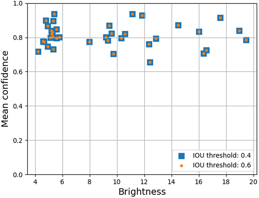
Figure 9. Brightness versus mean confidence of predictions for each video in the test set for YOLOv4 model trained with 2,000 samples in each class evaluated at IoU thresholds of 0.4 and 0.6.
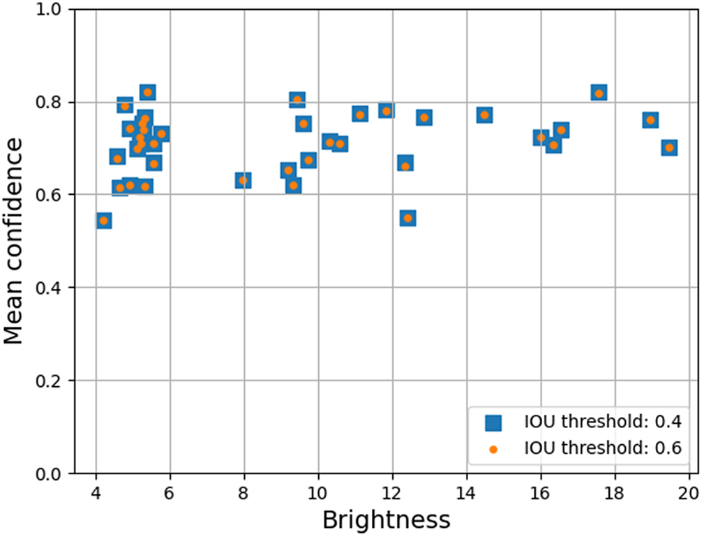
Figure 10. Brightness versus mean confidence of predictions for each video in the test set for YOLOv7 model trained with 2,000 samples in each class evaluated at IoU thresholds of 0.4 and 0.6.
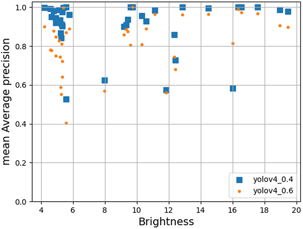
Figure 11. Brightness versus mAP of predictions for each video in the test set for YOLOv4 model trained with 2,000 samples in each class evaluated at IoU thresholds of 0.4 and 0.6.

Figure 12. Brightness versus mAP of predictions for each video in the test set for YOLOv7 model trained with 2,000 samples in each class evaluated at IoU thresholds of 0.4 and 0.6.
Surprisingly, we observed that neither the confidence nor the mAP of the detections appears to be influenced by the brightness of the videos. These results suggest that the trained models are robust enough to extract features from low-brightness videos and match them with the features learned during training to efficiently perform the task of classifying and detecting fish.
4. Discussion
We observe that YOLOv4 models have higher mAP, higher confidence values, and detect fewer false positives on water frames at low IoU thresholds; while YOLOv7 models detect a larger number of fish with more precise fish locations. YOLOv7 is a relatively recent revision of the YOLO family of models, which is written in Python, easier to use, and has ongoing community support. As such, we recommend choosing YOLOv7 for the detection and classification of fish with underwater cameras, because a larger number of highly precise detections are preferred for most applications. For applications where larger mAP and confidence values take more precedence, YOLOv4 could be a more preferable choice.
Although our models trained with the entire dataset performed best, our results demonstrate that models trained with 1,000 and 2,000 images per species performed with only a small loss of accuracy. Annotating image data with position and species information requires significant time and effort by trained experts so reducing this burden is necessary to enable the widespread use of this technology. We recommend that for an underwater dataset such as this, at least 2,000 samples in each class are preferred to train a YOLO family of models for good detection performance. Moreover, deep learning models learn from the data distribution they are trained on, so it is crucial that the 2,000 frames sampled from each class reflect variations in brightness and background habitat. This is especially important in the case of video data, as very little variation in image properties like brightness, contrast, and background is typically observed in frames sampled from the same video. As such, we recommend randomly sampling images from multiple videos when training such models to capture variations in the dataset. Finally, it is worth noting that the number of images required to train machine learning models may vary depending on the number of species in the dataset. Still, we recommend starting with 2,000 samples per species and scaling the number as necessary.
Surprisingly, we observed that the performance of our trained models was not affected by the brightness of the videos which dimmed over time as the batteries drained. One possible explanation is that the image augmentations used during the training of these models may have helped train models that are robust to some percentage of brightness variation. This provides an opportunity as recent research shows that bright light affects underwater ecosystems and may prevent some species of fish from casting anchor while attracting other unwanted species of fish with negative impacts on human and local marine communities (Davies et al., Reference Davies, Coleman, Griffith and Jenkins2015). We recommend that future deployments and possible systems consider light sources that emit low light to minimize disruption to local marine ecosystems in the region.
5. Future Work
We demonstrated that YOLO-based models can detect and classify fish species 500 m underwater given a sufficient number of training examples. However, such datasets naturally have large class imbalances (e.g., our excluded species: Whelk and Unknown) because the ocean floor is sparsely populated by fish, and fish species are unevenly distributed. An automated system for monitoring rare at-risk species will require models that can (a) efficiently classify species with as little as a single unique instance and (b) detect and catalog species the model has not previously seen. Toward this goal, we propose exploring an R-CNN family (Girshick et al., Reference Girshick, Donahue, Darrell and Malik2014; Sun et al., Reference Sun, Zhang, Jiang, Kong, Xu, Zhan, Tomizuka, Li, Yuan, Wang and Luo2021) model to train classifiers and detectors separately: training the detector to segment fish, freezing the detector’s layers; and training classifiers using small balanced subsets from identified species. Furthermore, we propose experiments augmenting the sample size of rarer species using generative models (Goodfellow et al., Reference Goodfellow, Pouget-Abadie, Mirza, Xu, Warde-Farley, Ozair, Courville and Bengio2014; Eom and Ham, Reference Eom and Ham2019; Karras et al., Reference Karras, Laine and Aila2019), optimizing training by subsampling efficiently to use all the training data while using balanced subsets, using statistical methods like joint probabilistic data association filters (He et al., Reference He, Shin and Tsourdos2017) to track and count fish across frames, and training with water frames to develop an efficient population estimation algorithm. Conducting before/after light experiments using echo sounders to better understand the effects of light on marine life, and combining different sensory spaces like light and sound to detect and classify fish species using machine learning could significantly augment marine conservation efforts by providing means to non-invasively monitor marine ecosystems. Marine conservation research using deep underwater video data has incredible potential if the enormous and expensive manual effort of labeling data can be reduced or replaced by machine learning strategies like one-shot or few-shot learning, leveraging large foundation models and using acoustics combined with video to aid classification and detection.
6. Conclusion
In addition to machine learning model development, there are several large challenges that must be solved to deploy automated analysis and continuous monitoring camera systems deep underwater on a large scale: replenishing/circumventing using bait to attract fish to the camera; limited on-chip data storage, resources to store and process large amounts of data; trained interdisciplinary scientists and operators to acquire and process the data; verification and generalisability to variations in habitat, camera resolutions, to name a few. We see this research, with its immediate extensibility to count and estimate populations, as the first step toward the larger goal of worldwide monitoring of life underwater which will require a concerted effort from multiple diverse groups including experts in machine learning, biology, and oceanography as well as social scientists. Interdisciplinary research projects fostering collaboration between social scientists and Indigenous peoples to develop and monitor programs that incorporate both scientific and traditional ecological knowledge can lead to more holistic and sustainable approaches to marine resource management, which can benefit both the environment and the communities that depend on it. If successful, such research may help enable the safe development of tidal power, safe development and application of carbon removal technology, better monitoring of at-risk fish in marine protected areas, and other upcoming solutions to help address our climate threat.
Acknowledgments
We wish to thank Faerie Mattins for discussions about differences between YOLO family models and their application to fish (Mattins and Whidden, Reference Mattins and Whidden2022). This research was enabled in part by computing resources provided by DeepSense, ACENET, and the Digital Research Alliance of Canada.
Author contribution
Conceptualization: C.M, J.B, C.W; Data curation: C.M, J.B; Formal analysis: D.A; Funding acquisition: C.M, J.B, C.W; Methodology: D.A, C.M, J.B, C.W; Project administration: C.W; Resources: C.W, C.M, J.B; Software: D.A; Supervision: C.W; Validation: D.A; Visualization: D.A; Writing—original draft: D.A; Writing—review & editing: C.W. All the authors have approved the final submitted draft.
Competing interest
The authors declare none.
Data availability statement
The data that support the findings of this study are available from DFO but restrictions apply to the availability of these data, which were used under license for the current study, and so are not publicly available. Data are however available from the authors upon reasonable request and with permission of DFO.
Ethics statement
The data is collected by DFO under applicable approvals and guidelines, and the research meets all ethical guidelines, including adherence to the legal requirements of the study country.
Funding statement
This research was supported by grants from National Research Council of Canada(NRC) (OCN-110-2) and Ocean Frontier Institute(OFI) (OG-202110). Data was provided by the Department of Fisheries and Oceans (DFO). CW is supported by a Natural Sciences and Engineering Research Council of Canada (NSERC) Discovery Grant (RGPIN-2021-02988).
Provenance statement
A preliminary version of this work appeared in the NeurIPS Climate Change Workshop (Ayyagari et al., Reference Ayyagari, Whidden, Morris and Barnes2022).


 Open access