


Impact Statement
This study presents CropGym, an open simulation environment to conduct reinforcement learning research for discovering adaptive, data-driven policies for farm management using a variety of process-based crop growth models. With a use case on nitrogen management, we demonstrate the potential of RL to learn sustainable policies that are competitive with standard practices set by domain experts.
1. Introduction
In recent years, smart farming technologies have been considered key enablers to reduce the usage of chemicals (fertilizers and plant protection products) and to reduce greenhouse gas emissions to enable reaching the Green Deal targets (Saiz-Rubio and Rovira-Más, Reference Saiz-Rubio and Rovira-Más2020). A promising direction within smart farming technology research focuses on developing decision support systems (DSSs). These human–computer systems aim at providing farmers with a list of advice for supporting their business or organizational decision-making activities to optimize returns on inputs while preserving resources, within (environmental) constraints. With the evolution of agriculture into Agriculture 4.0, thanks to the employment of current technologies such as Internet of things, remote sensing, big data, and artificial intelligence, DSSs of various kinds have found their way into agriculture. Examples include, but are not limited to, applications for agricultural mission planning, climate change adaptation, food waste control, plant protection, and resource management of water and nutrients (Zhai et al., Reference Zhai, Martínez, Beltran and Martínez2020).
The backbone of a DSS typically consists of a set of models that provide a representation of the environment and processes therein that are to be optimized. In particular, for resource management a substantial share of DSSs is based on process-based crop growth models (Graeff et al., Reference Graeff, Link, Binder and Claupein2012). These models mathematically describe the growth, development, and yield of a crop for given environmental conditions, such as type of soil, weather, and availability of water and nutrients. The scientific community offers numerous crop growth models with different levels of sophistication, limitations, and limits of applicability (Di Paola et al., Reference Di Paola, Valentini and Santini2016; Jones et al., Reference Jones, Antle, Basso, Boote, Conant, Foster, Godfray, Herrero, Howitt, Janssen, Keating, Munoz-Carpena, Porter, Rosenzweig and Wheeler2017). Widely used frameworks are APSIM (Holzworth et al., Reference Holzworth, Huth, deVoil, Zurcher, Herrmann, McLean, Chenu, van Oosterom, Snow, Murphy, Moore, Brown, Whish, Verrall, Fainges, Bell, Peake, Poulton, Hochman, Thorburn, Gaydon, Dalgliesh, Rodriguez, Cox, Chapman, Doherty, Teixeira, Sharp, Cichota, Vogeler, Li, Wang, Hammer, Robertson, Dimes, Whitbread, Hunt, van Rees, McClelland, Carberry, Hargreaves, MacLeod, McDonald, Harsdorf, Wedgwood and Keating2014), DSSAT (Jones et al., Reference Jones, Hoogenboom, Porter, Boote, Batchelor, Hunt, Wilkens, Singh, Gijsman and Ritchie2003), and PCSE (de Wit, Reference de Wit2023), which contain models such as LINTUL-3 (Shibu et al., Reference Shibu, Leffelaar, Van Keulen and Aggarwal2010) and WOFOST (de Wit et al., Reference de Wit, Boogaard, Fumagalli, Janssen, Knapen, van Kraalingen, Supit, van der Wijngaart and van Diepen2019).
Generally speaking, there are two major ways in which crop growth models are utilized in a DSS to derive crop management decisions (Gallardo et al., Reference Gallardo, Elia and Thompson2020): (1) Components in the model are exploited to provide estimates of crop yield-limiting factors, such as (future) deficiencies of nutrients and water, and (2) the model is employed as a specialized simulator to assess the impact of a set of (predefined) crop management practices. For both cases, it is not trivial to find the optimal set of actions, as decisions have to be made under uncertainty. For instance, driving factors for, for example, future nutrient uptake, such as future weather conditions, are uncertain at the time the model is asked for advice on fertilizer application.
Finding an optimized sequence of (crop management) decisions under uncertainty is a challenging task for which machine learning has increasingly been leveraged. In particular, reinforcement learning (RL), a subfield of machine learning, seems a relevant tool to tackle agricultural optimization problems (Binas et al., Reference Binas, Luginbuehl and Bengio2019). RL seeks to train intelligent agents in a trial-and-error fashion to take actions in an environment based on a reward signal. In RL, the environment is formally specified as a Markov decision process (MDP) $ \left\{S,A,T,R\right\} $
, with state space
$ \left\{S,A,T,R\right\} $
, with state space $ S $
, an available set of actions
$ S $
, an available set of actions $ A $
, a transition function
$ A $
, a transition function $ T $
, and a reward function
$ T $
, and a reward function $ R $
. In the context of, for example, crop management,
$ R $
. In the context of, for example, crop management, $ S $
may consist of (virtual) measurements on the state of the crop,
$ S $
may consist of (virtual) measurements on the state of the crop, $ A $
may be dose of fertilizer to apply,
$ A $
may be dose of fertilizer to apply, $ T $
may be represented by a simulation step of a crop growth model, and
$ T $
may be represented by a simulation step of a crop growth model, and $ R $
may be defined as the (projected) amount of yield.
$ R $
may be defined as the (projected) amount of yield.
Recently, a few research works have introduced RL for the management of agricultural systems. For instance, RL has been used for climate control in a greenhouse (Wang et al., Reference Wang, He and Luo2020), planting, and pruning in a polyculture garden (Avigal et al., Reference Avigal, Wong, Presten, Theis, Aeron, Deza, Sharma, Parikh, Oehme, Carpin, Viers, Vougioukas and Goldberg2022), fertilizer (Overweg et al., Reference Overweg, Berghuijs and Athanasiadis2021) and/or water management (Chen et al., Reference Chen, Cui, Wang, Xie, Liu, Luo, Zheng and Luo2021; Tao et al., Reference Tao, Zhao, Wu, Martin, Harrison, Ferreira, Kalantari and Hovakimyan2022; Saikai et al., Reference Saikai, Peake and Chenu2023), coverage path planning (Din et al., Reference Din, Ismail, Shah, Babar, Ali and Baig2022), and crop planning (Turchetta et al., Reference Turchetta, Corinzia, Sussex, Burton, Herrera, Athanasiadis, Buhmann and Krause2022) in open-field agriculture. A comprehensive overview of reinforcement learning for crop management support is given in Gautron et al. (Reference Gautron, Maillard, Preux, Corbeels and Sabbadin2022b).
As is common practice in RL research in a pioneering stage, practically all mentioned works used simulated environments. Some of these environments have been made publicly available as software artifact. Examples that build on crop growth models include CropGym (Overweg et al., Reference Overweg, Berghuijs and Athanasiadis2021), an interface to the Python Crop Simulation Environment (PCSE) (de Wit, Reference de Wit2023), gym-DSSAT (Gautron et al., Reference Gautron, Gonzalez, Preux, Bigot, Maillard and Emukpere2022a), an integration of the DSSAT (Hoogenboom et al., Reference Hoogenboom, Porter, Boote, Shelia, Wilkens, Singh, White, Asseng, Lizaso and Patricia Moreno2019) crop models, CropRL (Ashcraft and Karra, Reference Ashcraft and Karra2021), a wrapper around the SIMPLE crop model (Zhao et al., Reference Zhao, Liu, Xiao, Hoogenboom, Boote, Kassie, Pavan, Shelia, Kim and Hernandez-Ochoa2019), SWATGym (Madondo et al., Reference Madondo, Azmat, DiPietro, Horesh, Jacobs, Bawa, Srinivasan and O’Donncha2023), a wrapper around SWAT (Arnold et al., Reference Arnold, Kiniry, Srinivasan, Williams, Haney and Neitsch2011), and CyclesGym (Turchetta et al., Reference Turchetta, Corinzia, Sussex, Burton, Herrera, Athanasiadis, Buhmann and Krause2022), a wrapper around Cycles (Kemanian et al., Reference Kemanian, White, Shi, Stockle and Leonard2022). The mentioned examples are implemented with the Gymnasium toolkit (Towers et al., Reference Towers, Terry, Kwiatkowski, Balis, Cola, Deleu, Goulão, Kallinteris, Arjun, Krimmel, Perez-Vicente, Pierré, Schulhoff, Tai, Shen and Younis2023), which is a highly used framework for developing and comparing reinforcement learning algorithms. By providing standardized test beds, efforts like these are instrumental in further promoting and accelerating RL research for agricultural problems.
In this study, we present the development of CropGym, a Gymnasium environment, where a reinforcement learning agent can learn farm management policies using a variety of process-based crop growth models. In particular, we report on the discovery of strategies for nitrogen application in winter wheat and we evaluate the resiliency of the obtained policies against climate change. The focus on nitrogen is motivated by the fact that (in rain-fed winter wheat) nitrogen is a key driver for yield, yet if supplied in excessive amount it has a detrimental effect on the environment, including eutrophication of freshwater, groundwater contamination, tropospheric pollution related to emissions of nitrogen oxides and ammonia gas, and accumulation of nitrous oxide, a potent greenhouse gas (Zhang et al., Reference Zhang, Davidson, Mauzerall, Searchinger, Dumas and Shen2015).
2. Methodology
2.1. CropGym
We developed CropGym, a Gymnasium environment, for farm management policies, such as fertilization and irrigation, using process-based crop growth models. CropGym is built around the Python Crop Simulation Environment (PCSE), a well-established open-source framework that includes implementations of a variety of crop simulation models. The software is characterized by a high level of customizability. Input parameters, such as crop characteristics, are easily configurable. For deriving driving variables, such as weather information, a broad selection of sources is available. Furthermore, dedicated routines facilitate the assimilation of observational data, such as field measurements. State parameters on crop growth and development, as well as carbon, water, and nutrient balances, are simulated and outputted at daily time steps. Farm management actions can be applied at the same resolution.
CropGym follows standard gym conventions and enables daily interactions between an RL agent and a crop model. The code is designed in a modular fashion and allows users to flexibly and easily create custom environments. Users can, for example, base action and reward functions on crop state variables, such as water stress, nitrogen uptake, and biomass. As a backbone, a variety of (components of) crop growth models can be selected or combined. CropGym is shipped with a set of preconfigured environments that allow for readily conducting RL research for farm management practices. The source code and documentation are available at https://www.cropgym.ai.
2.2. Use case
In this work, we present a use case on nitrogen management in rain-fed winter wheat. An agent was trained to decide weekly on applying a discrete amount of nitrogen fertilizer, with the goal of balancing the trade-off between yield and environmental impact.
In the following, we outline the components that comprise the environment of our use case.
State space S consists of the current state of the crop and a multidimensional weather observation, as parameterized with the variables listed in Table 1.
Table 1. Crop growth and weather variables exposed in the state space $ S $
$ S $

Action space A comprises three possible fertilizer application amounts, namely {0, 20, 40} kg/ha.
Reward function R constitutes the balance between the gain in yield and the (environmental) costs associated with the application of nitrogen. $ R $
is formalized as follows:
$ R $
is formalized as follows:
 $$ {r}_t=({WSO}_t^{\pi }-{WSO}_{t-1}^{\pi })-({WSO}_t^0-{WSO}_{t-1}^0)-\beta {N}_t, $$
with $ t $
the timestep,
$ t $
the timestep, $ WSO $
the weight of the storage organ (g/m2), and
$ WSO $
the weight of the storage organ (g/m2), and $ N $
the amount of nitrogen (g/m2). The upper indices π and 0 refer to the agent’s policy and a zero nitrogen policy, respectively. Parameter
$ N $
the amount of nitrogen (g/m2). The upper indices π and 0 refer to the agent’s policy and a zero nitrogen policy, respectively. Parameter $ \beta $
determines the trade-off between increased yield and reduced environmental impact. Setting
$ \beta $
determines the trade-off between increased yield and reduced environmental impact. Setting $ \beta \approx 2.0 $
corresponds to a reward that purely comprises economic profitability, since a kg of fertilizer is twice as expensive as a kg of wheat (Agri23a, 2023; Agri23b, 2023). In this work, we present results for
$ \beta \approx 2.0 $
corresponds to a reward that purely comprises economic profitability, since a kg of fertilizer is twice as expensive as a kg of wheat (Agri23a, 2023; Agri23b, 2023). In this work, we present results for $ \beta =10.0 $
to emphasize the environmental costs.
$ \beta =10.0 $
to emphasize the environmental costs.
Transitions are governed by the process-based crop model LINTUL-3 (light interception and utilization (Shibu et al., Reference Shibu, Leffelaar, Van Keulen and Aggarwal2010)) and the weather sequence. The model parameters have been calibrated to simulate winter wheat in the Netherlands (Wiertsema, Reference Wiertsema2015; Berghuijs et al., Reference Berghuijs, Silva, Rijk, van Ittersum, van Evert and Reidsma2023). Weather data were obtained from the PowerNASA database for three locations in the Netherlands and one in France for the years 1990 to 2022. An episode runs until the crop has reached maturity, which differs between episodes because of weather conditions.
An RL agent was trained with proximal policy optimization (PPO) (Schulman et al., Reference Schulman, Wolski, Dhariwal, Radford and Klimov2017) as implemented in the Stable-Baselines3 library (Raffin et al., Reference Raffin, Hill, Gleave, Kanervisto, Ernestus and Dormann2021). The environment was normalized with the VecNormalize environment wrapper, a normalized reward, and observation clipping set to 10. The discount factor $ \gamma $
was set to 1.0 as we aim to optimize the cumulative reward over the entire episode. To reduce redundancy among the input data, we aggregated the time-series data: The weather sequence, with size of 3x7 (i.e., features x days), was processed with an average pooling layer, yielding a feature vector of size of 3x1. The crop features, with size of 9x7, were shrunk to 9x1, by taking the last entry for each feature. Both resulting feature vectors were concatenated and subsequently flattened to obtain a feature vector of size of 12. The policy and the value network were a multilayer perceptron with two hidden layers, each of size of 128, and activation function
$ \gamma $
was set to 1.0 as we aim to optimize the cumulative reward over the entire episode. To reduce redundancy among the input data, we aggregated the time-series data: The weather sequence, with size of 3x7 (i.e., features x days), was processed with an average pooling layer, yielding a feature vector of size of 3x1. The crop features, with size of 9x7, were shrunk to 9x1, by taking the last entry for each feature. Both resulting feature vectors were concatenated and subsequently flattened to obtain a feature vector of size of 12. The policy and the value network were a multilayer perceptron with two hidden layers, each of size of 128, and activation function $ \tanh $
. Weights were shared between both networks. The training was done on the odd years from 1990 to 2022 (the even years were reserved for validation), with weather data from (52,5.5), (51.5,5), and (52.5,6.0) (°N,°E). The training ran for 400,000 timesteps using default hyperparameters. We selected PPO as our choice of RL algorithm due to its consistent high performance in RL research and its robust nature (Schulman et al., Reference Schulman, Wolski, Dhariwal, Radford and Klimov2017). We also explored training a Deep Q-Network (DQN) (Mnih et al., Reference Mnih, Kavukcuoglu, Silver, Graves, Antonoglou, Wierstra and Riedmiller2013), which yielded similar results to those obtained (see Appendix A).
$ \tanh $
. Weights were shared between both networks. The training was done on the odd years from 1990 to 2022 (the even years were reserved for validation), with weather data from (52,5.5), (51.5,5), and (52.5,6.0) (°N,°E). The training ran for 400,000 timesteps using default hyperparameters. We selected PPO as our choice of RL algorithm due to its consistent high performance in RL research and its robust nature (Schulman et al., Reference Schulman, Wolski, Dhariwal, Radford and Klimov2017). We also explored training a Deep Q-Network (DQN) (Mnih et al., Reference Mnih, Kavukcuoglu, Silver, Graves, Antonoglou, Wierstra and Riedmiller2013), which yielded similar results to those obtained (see Appendix A).
Two baseline agents were implemented as a reference for the RL agent:
The standard practice agent (SP) applies a fixed amount of nitrogen that is the same for all episodes. SP thereby reflects common practice, in which a predetermined amount of nitrogen is applied on three different dates during the season (Wiertsema, Reference Wiertsema2015). The static amount of nitrogen SP applied is determined by the optimizationFootnote 1 on the training set.
The Ceres agent applies an episode-specific amount of nitrogen, that is optimizedFootnote 1 for the episode it is evaluated on. Effectively, Ceres has access to the weather data of the entire season, which contrasts with the RL agent that only has access to current and past weather data. Ceres can thus base its actions on future weather conditions and thereby reflects the upper bound of what any agent can achieve maximally.
We evaluated the performance of the implemented agents in the even years from 1990 to 2022 with weather data from (52,5.5) (°N,°E). As performance metrics, we computed the cumulative reward, the amount of nitrogen, and the yield, summarized as the median over the test years. For statistical analyses, we performed 15 runs initialized with different seeds and used bootstrapping to estimate the 95% confidence interval around the median.
As an out-of-distribution test, we evaluated the resiliency of the policy against a change in climate conditions. For that, we deployed both the trained RL and the baseline agents in a more southern climate. Practically, this was implemented by taking weather data from (48,0.0) (°N, °E), located in France, as opposed to (48,0.0) (°N, °E), located in the Netherlands, used during training (see Figure 1).

Figure 1. Locations of the training (red) and out-of-distribution test (blue), with a CCAFS climate similarity index (Villegas et al., Reference Villegas, Lau, Köhler, Jarvis, Arnell, Osborne and Hooker2011) of 1.0 (reference) and 0.573, respectively.
To reestablish the upper bound, Ceres was tuned to the weather data from the southern climate; SP and RL were not retrained. The robustness of the RL (and SP) agents was evaluated by assessing how close the agents’ performance remains to the optimum, as determined by Ceres.
3. Results
A reinforcement learning agent (RL) was trained to find the optimal policy for applying nitrogen that balances yield increase and (environmental) costs. Two baseline agents were implemented for comparison: (1) The standard practice agent (SP) applies a fixed amount of nitrogen that does not differ between episodes and (2) the Ceres agent applies an episode-specific amount of nitrogen. The amount of nitrogen SP applied is determined by the optimization of the training set. Ceres, however, applies an amount of nitrogen that is optimized for the episode it is evaluated on. Ceres thereby reflects the upper bound of what any agent can achieve maximally.
Table 2 reports the performance metrics for each of the three agents, summarized as the median over the test years, and its associated 95% confidence interval. The amount of nitrogen the RL agent applies, and the resulting yield and cumulative reward are close to the upper bound, as reflected by Ceres. Comparing the RL agent with the standard practice (SP), we see that RL applies more nitrogen, which results in a higher yield. The cumulative reward RL achieves is competitive with SP.
Table 2. Cumulative reward, nitrogen, and yield (median and associated 95% CI)
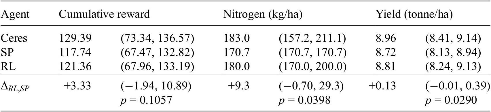
Figure 2 (left and middle) shows for each test year the reward obtained and amount of nitrogen applied by each of the three agents, as a function of the reward obtained and amount of nitrogen applied by Ceres. For most test years, RL is closer to Ceres than SP, in terms of both obtained cumulative reward and applied nitrogen. For two test years (2006 and 2010), the optimal amount of nitrogen, as determined by Ceres, is zero. In these years, which are characterized by a low amount of rainfall, the extra yield obtained by applying nitrogen does not outweigh the costs. RL (and SP) fail(s) to limit the nitrogen application, however, resulting in negative cumulative rewards. Figure 2 (right) shows for each test year the difference in yield between the RL agent and the SP agent, as a function of the difference in invested nitrogen. The diagonal shows the break-even line, for which the difference in reward is zero. Most test years, as well as the median, are above the break-even line, demonstrating that the RL agent’s decision to apply a different amount of nitrogen is adequate.
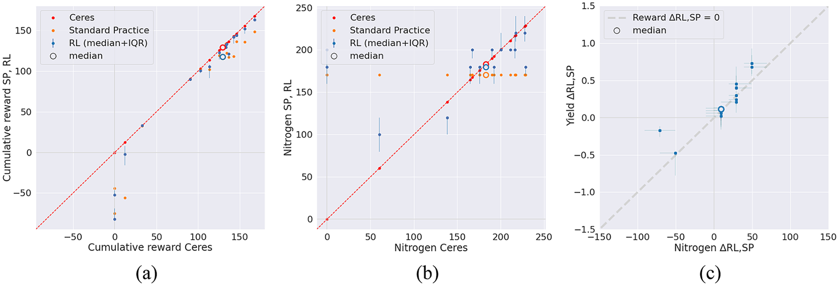
Figure 2. (a): Cumulative reward obtained and (b): nitrogen applied by each of the three agents. Each dot depicts a test year (n=16). For most test years, RL is closer to Ceres than SP. (c): the difference in yield between the RL agent and the SP agent as a function of the difference in the amount of nitrogen applied. The dashed line indicates the break-even line, at which both agents achieve the same reward. Most test years are above the break-even line, demonstrating that the RL agent’s choice of applying a different amount of nitrogen is adequate.
Figure 3 shows the evolvement of the actions and rewards of the RL agent during the growing season, as summarized by the median over the test years. Typically, the RL agent waits until spring for its first actions. The median number of fertilization events is 7.0 (95% CI 6.0–8.0). The median length of an episode is 208 days (95% CI 205–211).
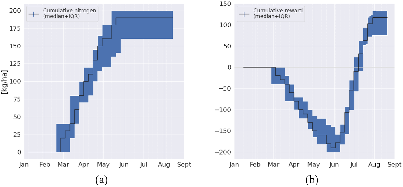
Figure 3. Policy visualization of the RL agent: (a) cumulative reward obtained and (b) nitrogen applied. Typically, the RL agent waits until spring for its first actions.
The main driver for applying nitrogen is rainfall. Pearson’s correlation coefficient between the total amount of rainfall during the growing season and the total amount of nitrogen applied is 0.69 (95% CI 0.58–0.76) for Ceres and 0.63 (95% CI 0.12–0.82) for RL (see Figure 4).

Figure 4. Scatter plot with regression lines of the average daily rainfall and the total amount of nitrogen applied by all three agents for (a) the northern climate and (b) the southern climate. The optimal amount of nitrogen, as determined by Ceres, depends substantially on rainfall. Presumably, the RL agent has learned to adopt this general trend. In dry years, when lack of rainfall impairs yield and the optimal amount of nitrogen is (close to) zero, the RL agent does not limit its nitrogen application sufficiently, as it arguably sticks to the general trend. In years with sufficient rainfall, the RL agent acts in line with the optimal policy. This effect is seen in both the northern climate and the southern climate.
3.1. Climate resilience
To assess the robustness of the learned policy against changing climate conditions, we deployed both the trained RL and the baseline agents in a more southern climate. With a climate similarity index of 0.573, as determined with the CCAFS method (Villegas et al., Reference Villegas, Lau, Köhler, Jarvis, Arnell, Osborne and Hooker2011), using average temperature and precipitation as weather variables, the southern climate differs substantially from the northern climate. The southern climate is characterized by a higher average temperature (10.4 °C vs 9.8 °C), less amount of average daily rainfall (1.92 mm vs 2.12 mm), and a shorter growing season (200 days vs 208 days).
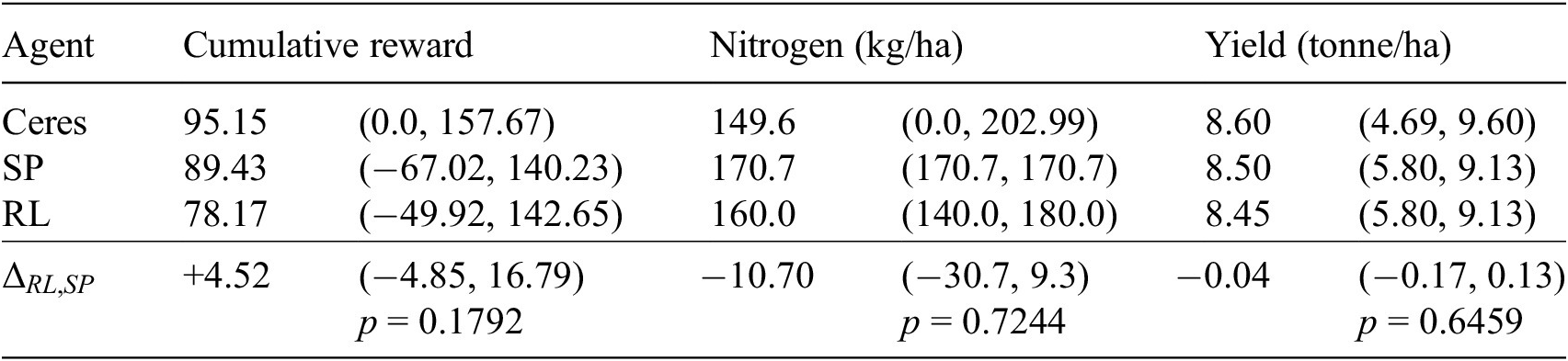
Table 3 reports the performance metrics for each of the three agents deployed in the southern climate. The maximally achievable cumulative reward and yield, as represented by Ceres, are lower than what is obtained in the northern climate. In six years, namely 1990, 1992, 1996, 2004, 2006, and 2010, yield is (partially) limited by a low amount of rainfall, resulting in low cumulative rewards. In these dry years, the performance of the RL agent is suboptimal, as it does not limit its nitrogen application sufficiently. Yet, the cumulative reward RL achieves is competitive with SP. In years with sufficient rainfall, the RL agent remains close to the optimal policy, as is illustrated in Figure 4, just as we saw for the northern climate.
Table 3. Out-of-distribution results: cumulative reward, nitrogen, and yield (median and 95% CI) in southern climate
4. Discussion
We presented CropGym, a Gymnasium environment, to study policies for farm management, such as fertilization and irrigation, using process-based crop growth models. We developed a use case on nitrogen fertilization in rain-fed winter wheat. A reinforcement learning agent was trained to find the optimal timings and amounts for applying nitrogen that balance yield and environmental impact. The agent was found to learn close to optimal strategies, competitive with standard practices set by domain experts.
As an out-of-distribution test, we evaluated whether the obtained policies were resilient against a change in climate conditions, with sound results. Yet, in years where yield is limited by a shortage of rainfall, the performance of the RL agent was suboptimal. The adoption of more dry weather data in the training through, for example, fine-tuning approaches, may improve these results. Other examples of out-of-distribution tests with practical impact include variations in soil characteristics, such as organic matter content.
Clearly, as is common in RL research, our experiments are done in silico, and it is an open question to what extent our results transfer into the real world. (Crop growth) models are by definition simplifications of reality, and thus, policies derived from these models are inherently subject to a simulation-to-reality gap. Narrowing this gap can be achieved by employing an ensemble of different crop growth models (Wallach et al., Reference Wallach, Martre, Liu, Asseng, Ewert, Thorburn, van Ittersum, Aggarwal, Ahmed, Basso, Biernath, Cammarano, Challinor, De Sanctis, Dumont, Rezaei, Fereres, Fitzgerald, Gao, Garcia-Vila, Gayler, Girousse, Hoogenboom, Horan, Izaurralde, Jones, Kassie, Kersebaum, Klein, Koehler, Maiorano, Minoli, Müller, Kumar, Nendel, O’Leary, Palosuo, Priesack, Ripoche, Rötter, Semenov, Stöckle, Stratonovitch, Streck, Supit, Tao, Wolf and Zhang2018). CropGym supports such a strategy by offering implementations of a variety of process-based crop growth models.
To further bridge the gap between simulation and reality, digital twin technology could be exploited (Pylianidis et al., Reference Pylianidis, Osinga and Athanasiadis2021). A variety of sensors can be employed to synchronize digital representations of crops with their physical counterparts (Jin et al., Reference Jin, Kumar, Li, Feng, Xu, Yang and Wang2018; Jindo et al., Reference Jindo, Kozan and de Wit2023). Yet, the acquisition of sensor data may come with high (monetary) costs. In this context, CropGym could be utilized to train agents that are able to determine when and to what extent the environment should be measured (Bellinger et al., Reference Bellinger, Drozdyuk, Crowley and Tamblyn2021). In such a training, the agent chooses between either relying on the simulated state of the crop or paying the cost to measure the true state and update the crop growth model accordingly.
In this work, we incentivize the RL agent to generate environmentally friendly policies by negotiating the environmental costs of nitrogen application in the reward function. An alternative approach would be to set hard constraints on the total amount of nitrogen applied. Such could be achieved by building on the works in the domain of (safety)-constrained RL (Liu et al., Reference Liu, Halev and Liu2021), supported by, for example, OpenAI’s dedicated Safety Gym benchmark suite (Ray et al., Reference Ray, Achiam and Amodei2019). Another constraint that could be considered is the number of fertilization events.
As an open simulation environment, CropGym can be used to discover adaptive, data-driven policies that perform well across a range of plausible scenarios for the future. With CropGym, we aim to facilitate a joint research effort from the RL and agronomy communities to meet the challenges of future agricultural decision-making and to further match farmers’ decision-making processes.
Acknowledgments
The authors would like to thank Allard de Wit and Herman Berghuijs for the discussion and revision of the employed crop growth model and Lotte Woittiez for the constructive discussions during various stages of the research.
Author contribution
M.G.J.K., H.O., and I.N.A. conceptualized the study; M.G.J.K. and I.N.A. designed methodology; M.G.J.K., H.O., and R.v.B. provided software; M.G.J.K. visualized the data; M.G.J.K. and I.N.A. validated the data; M.G.J.K. wrote the original draft; H.O., R.v.B., and I.N.A. wrote, reviewed, and edited the article; and all authors approved the final submitted draft.
Competing interest
The authors declare none.
Data availability statement
Data and replication code can be found at https://www.cropgym.ai.
Ethics statement
The research meets all ethical guidelines, including adherence to the legal requirements of the study country.
Funding statement
This work has been partially supported by the European Union Horizon 2020 Research and Innovation program (Project Code: 101070496, Smart Droplets) and the Wageningen University and Research Investment Programme “Digital Twins.”
A. Appendix. Results of DQN
In addition to training with PPO, we explored training a Deep Q-Network (DQN) (Mnih et al., Reference Mnih, Kavukcuoglu, Silver, Graves, Antonoglou, Wierstra and Riedmiller2013). Configurations were kept the same as with PPO. We used the default settings of the (hyper)parameters, as set by Stable Baselines, except for (1) the number of hidden units, which was set to 128x128, (2) the activation function, which was set to $ \tanh $
, and (3) exploration_final_eps, which was set to 0.01. The training ran for 400,000 timesteps.
$ \tanh $
, and (3) exploration_final_eps, which was set to 0.01. The training ran for 400,000 timesteps.
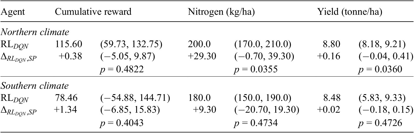
Below, we report the key results, aggregated over five runs with different random seeds. Figure 5 demonstrates that for each test year (a) the cumulative reward, (b) the amount of fertilizer, and (c) the yield obtained by the DQN agent closely resemble those of the PPO agent. Table 4 shows that, similar to $ {RL}_{PPO} $
, also
$ {RL}_{PPO} $
, also $ {RL}_{DQN} $
achieves results competitive with SP.
$ {RL}_{DQN} $
achieves results competitive with SP.

Figure 5. Scatter plot of PPO and DQN agent for (a): cumulative reward obtained, (b): nitrogen applied, and (c): yield obtained. Each point depicts a test year (n = 32).
Table 4. Cumulative reward, nitrogen, and yield (median and associated 95% CI) for DQN


 Open access