Impact Statement

Acute surface-level ozone events have a multitude of negative health consequences. Meteorology plays a major role in the development and intensification of these events; therefore, better understanding the complex interplay between meteorology and surface-level ozone is paramount. For this purpose, in this work, we develop a methodology to model the relationship between vertical temperature profiles and high quantiles of surface-level ozone. We find that acute surface-level ozone events are associated with air temperature inversions over much of the US Southwest in the summer; however, hot weather conditions look to be the primary driver over the Sierra Nevada Mountains and in far Northern California.

2. Pointwise Functional Quantile Regression Modeling

For the random process $ \left\{Y,\boldsymbol{X}\right\} $ with iid copies $ {\left\{{Y}_t,{\boldsymbol{X}}_t\right\}}_{t\in \mathrm{\mathbb{N}}} $ , assume the response variable of interest is $ {Y}_t\in \mathrm{\mathbb{R}} $ , and $ {\boldsymbol{X}}_t:\left[0,H\right]\to \mathrm{\mathbb{R}} $ is a functional covariate. Further, assume that $ {\left\{{X}_t\right\}}_{t\in \mathrm{\mathbb{N}}} $ are in $ {\mathrm{\mathcal{L}}}^2 $ , the separable Hilbert space determined by the set of measurable real-valued square-integrable functions on [0,H]. Given the value of the functional covariate, we directly model $ {Q}_{\tau}\left({Y}_t|{\boldsymbol{X}}_t\right) $ , the conditional $ \tau $ th quantile of the scalar response variable for some $ \tau \in \left(0,1\right) $ , via

(1) $$ {Q}_{\tau}\left({Y}_t|{\boldsymbol{X}}_t\right)\hskip0.35em =\hskip0.35em {\alpha}_{\tau }+{\int}_0^H{\boldsymbol{X}}_t^c(s){\boldsymbol{\beta}}_{\tau }(s) ds. $$

We note that the intercept $ {\alpha}_{\tau}\in \mathrm{\mathbb{R}} $ , and we call $ {\boldsymbol{X}}_t^c(s)\hskip0.35em =\hskip0.35em {\boldsymbol{X}}_t(s)-E\left(\boldsymbol{X}(s)\right) $ the centered covariate function. Additionally, the twice differentiable function $ {\boldsymbol{\beta}}_{\tau } $ is called the coefficient function for the $ \tau $ th quantile. In a typical analysis, estimation and inference regarding $ {\boldsymbol{\beta}}_{\tau } $ in equation (1) is a primary aim, as portions of $ \left[0,H\right] $ over which the coefficient function is positive (negative), imply a positive (negative) relationship with that conditional quantile of the response. Additionally, we assume that $ {\boldsymbol{\beta}}_{\tau}^{\prime \prime}\in {\mathrm{\mathcal{L}}}^2 $ , and that $ {\boldsymbol{\beta}}_{\tau } $ and $ {\boldsymbol{\beta}}_{\tau}^{\prime } $ are both absolutely continuous.

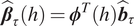
As this is commonly done in FDA, we assume that $ {\boldsymbol{\beta}}_{\tau } $ can be approximated by a linear combination of a finite set of known basis functions, $ {\left\{{\phi}_k\right\}}_{k=1,\dots, K} $ . This implies $ {\boldsymbol{\beta}}_{\tau }(s)\approx {\sum}_{k=1}^K{b}_k{\phi}_k(s)\hskip0.35em =\hskip0.35em {\boldsymbol{\phi}}^T(s){\mathbf{b}}_{\tau } $ . In reality, functional covariates $ {\left\{{\boldsymbol{x}}_i\right\}}_{i=1,\dots, n} $ are infinite dimensional and therefore not fully be observed. Instead, the analyst observes $ {\left\{{\boldsymbol{x}}_i(h)\right\}}_{i=1,\dots, n} $ for $ h\in \left\{{h}_1,\dots, {h}_U\right\} $ such that $ 0<{h}_1<\cdots <{h}_U\le H $ . We further assume that we are able to identify $ {\boldsymbol{a}}_i\in {\mathrm{\mathbb{R}}}^M $ such that $ {\boldsymbol{x}}_i(s)\approx {\sum}_{m=1}^M{a}_{i,m}{\psi}_m(h)={\boldsymbol{\psi}}^T(h){\boldsymbol{a}}_i $ , where $ {\left\{{\psi}_m\right\}}_{m=1,\dots, M} $ is another set of known basis functions. Therefore, the conditional quantile in equation (1) can be expressed via

(2) $$ {Q}_{\tau}\left({Y}_t|{\boldsymbol{X}}_t\right)\hskip0.35em \approx \hskip0.35em {\alpha}_{\tau }+{\int}_0^H\left({\boldsymbol{a}}_t^T\boldsymbol{\psi} (h)\right)\left({\boldsymbol{\phi}}^T(h){\boldsymbol{b}}_{\tau}\right) dh\hskip0.35em =\hskip0.35em {\alpha}_{\tau }+{\boldsymbol{a}}_t^T{\boldsymbol{Jb}}_{\tau }. $$

Here, the $ M\times K $ dimensional matrix $ \boldsymbol{J} $ is constructed such that the entry in the $ m $ th row and $ k $ th column is $ {\int}_0^H{\psi}_m(h){\phi}_k(h) dh $ . We estimate $ {\boldsymbol{b}}_{\tau } $ and $ {\alpha}_{\tau } $ via

(3) $$ {\left({\hat{\alpha}}_{\tau },{\hat{\boldsymbol{b}}}_{\tau}\right)}^T=\underset{\boldsymbol{b}\in {\mathrm{\mathbb{R}}}^K,\alpha \in \mathrm{\mathbb{R}}}{\mathrm{argmin}}\sum \limits_{t=1}^n{\rho}_{\tau}\left({y}_t-\alpha -{\boldsymbol{a}}_t^T\boldsymbol{Jb}\right), $$

where $ {\rho}_{\tau } $ is the check-loss function commonly used in quantile regression (Koenker and Bassett Jr., Reference Koenker and Bassett1978). The resulting optimum from equation (3) leads to the coefficient function estimator via the relationship $ {\hat{\boldsymbol{\beta}}}_{\tau }(h)={\boldsymbol{\phi}}^T(h){\hat{\boldsymbol{b}}}_{\tau } $ .

3. Functional Quantile Regression Modeling on a Grid

Climate scientists often make use of gridded data products, which can be thought of as producing output over the points on a regular spatial lattice. Assume that $ \mathcal{D} $ is a spatial domain of interest, and that we observe data over the set of points on a regular lattice $ {\mathcal{D}}^{\prime}\subset {\mathrm{\mathbb{Z}}}^2 $ , such that $ {\mathcal{D}}^{\prime}\subset \mathcal{D} $ . Despite the fact that the primary objective is to describe the association between the functional covariate and a key quantile of the scalar response everywhere in $ \mathcal{D} $ , we assume that modeling this relationship $ \mathrm{\forall}\ \mathbf{s}\in {\mathcal{D}}^{\mathrm{\prime}} $ will be useful. Additionally, we assume that the true coefficient functions at nearby locations are similar, which makes the approach of borrowing information from nearby cells a potentially promising way to improve coefficient function estimates.

Assume that at time $ t\in \left\{1,\dots, n\right\} $ , we observe realizations of a functional covariate and scalar response at locations $ {\left\{{\boldsymbol{s}}_l\right\}}_{l=1,\dots, L} $ such that $ {\boldsymbol{s}}_l\in {\mathcal{D}}^{\mathrm{\prime}}\ \mathrm{\forall}\ l\in \{1,\dots, L\} $ , at a sequence of pressure levels $ 0<{h}_1<\cdots <{h}_U\hskip0.35em \le \hskip0.35em H $ . We propose a procedure to simultaneously estimate all $ L $ coefficient functions $ {\left\{{\boldsymbol{\beta}}_{\tau, l}\right\}}_{l=1,\dots, L} $ , under the assumptions described above. We again assume that the true coefficient function at $ {\boldsymbol{s}}_l $ is well approximated by a finite linear combination of known basis functions, giving $ {\boldsymbol{\beta}}_{\tau, l}(h)\approx {\sum}_{k=1}^K{b}_{l,k,\tau }{\phi}_k(h)\hskip0.35em =\hskip0.35em {\boldsymbol{\phi}}^T(h){\boldsymbol{b}}_{l,\tau } $ . Observations from the functional covariate are denoted by $ {\left\{{\boldsymbol{x}}_{l,t}(h)\right\}}_{l\in \left\{1,\dots, L\right\},t\in \left\{1,\dots, n\right\}} $ , and assume further that there exists $ {\boldsymbol{a}}_{l,t}\in {\mathrm{\mathbb{R}}}^M $ such that $ {\boldsymbol{x}}_{l,t}(h)\approx {\sum}_{m=1}^M{a}_{l,t,m}{\psi}_m(h)\hskip0.35em =\hskip0.35em {\boldsymbol{\psi}}^T(h){\boldsymbol{a}}_{l,t} $ . We then approximate the conditional $ \tau $ th quantile of the response at time $ t $ and location $ {\boldsymbol{s}}_l $ by

(4) $$ {Q}_{\tau}\left({Y}_{l,t}|{\boldsymbol{X}}_{l,t}\right)\hskip0.35em \approx \hskip0.35em {\alpha}_{l,\tau }+{\int}_0^H\left({\boldsymbol{a}}_{l,t}^T\boldsymbol{\psi} (h)\right)\left({\boldsymbol{\phi}}^T(h){\boldsymbol{b}}_{l,\tau}\right) dh\hskip0.35em =\hskip0.35em {\alpha}_{l,\tau }+{\boldsymbol{a}}_{l,t}^T{\boldsymbol{Jb}}_{l,\tau }. $$

One could consider the estimator

(5) $$ {\left({\tilde{\boldsymbol{A}}}_{\tau}^T,{\tilde{\boldsymbol{B}}}_{\tau}^T\right)}^T=\underset{\boldsymbol{B}\in {\mathrm{\mathbb{R}}}^{KL},\boldsymbol{A}\in {\mathrm{\mathbb{R}}}^L}{\mathrm{argmin}}{\Lambda}_{\tau}\left({\boldsymbol{A}}_{\tau },{\boldsymbol{B}}_{\tau}\right), $$

for $ {\boldsymbol{A}}_{\tau }={\left({\alpha}_{1,\tau },\dots, {\alpha}_{L,\tau}\right)}^T $ and $ {\boldsymbol{B}}_{\tau }={\left({\boldsymbol{b}}_{1,\tau}^T,\dots, {\boldsymbol{b}}_{L,\tau}^T\right)}^T $ , where

(6) $$ {\Lambda}_{\tau}\left({\boldsymbol{A}}_{\tau },{\boldsymbol{B}}_{\tau}\right)=\sum \limits_{l=1}^L\left(\sum \limits_{t=1}^n{\rho}_{\tau}\left({y}_{tl}-{\alpha}_{l,\tau }-{\boldsymbol{a}}_{l,t}^T{\boldsymbol{Jb}}_{l,\tau}\right)\right). $$

The estimator in equation (5) does not incorporate any sort of penalty for dissimilarity between neighboring estimated coefficient functions. As we believe that nearby coefficient functions exhibit similarity in our data application, we supplement the loss function in equation (5) by an additional penalty term.

3.1. Penalizing spatial dissimilarity

Our spatial region of interest is composed of lush forests, arid deserts, coastal regions, and high mountain terrain. Because of this geographical heterogeneity, some pairs of neighboring cells on the lattice may exhibit a higher (or lower) degree of spatial similarity in terms of their true underlying coefficient functions. For this reason, for neighboring locations $ {\boldsymbol{s}}_l $ and $ {\boldsymbol{s}}_{l^{\prime }} $ ( $ l\ne {l}^{\prime } $ ), we propose the weighting function

(7) $$ {w}_{\theta, \gamma}\left({\boldsymbol{s}}_l,{\boldsymbol{s}}_{l^{\prime }}\right)=\theta \exp \left(-\gamma \delta \left({\boldsymbol{s}}_l,{\boldsymbol{s}}_{l^{\prime }}\right)\right), $$

where $ \theta >0 $ and $ \gamma \hskip0.35em \ge \hskip0.35em 0 $ are unknown parameters and the function $ \delta $ models geographic and or climatological dissimilarity between two locations. We propose the penalized estimator

(8) $$ {\left({\hat{\boldsymbol{A}}}_{\tau}^T,{\hat{\boldsymbol{B}}}_{\tau}^T\right)}^T=\underset{\boldsymbol{B}\in {\mathrm{\mathbb{R}}}^{KL},\boldsymbol{A}\in {\mathrm{\mathbb{R}}}^L}{\mathrm{argmin}}{\Lambda}_{\tau}\left(\boldsymbol{A},\boldsymbol{B}\right)+{\Lambda}_{\mathrm{spat}}\left(\boldsymbol{A},\boldsymbol{B},\theta, \gamma, \tau \right), $$

where $ {\Lambda}_{\tau } $ is defined in equation (6) and

(9) $$ {\Lambda}_{\mathrm{spat}}\left(\boldsymbol{A},\boldsymbol{B},\theta, \gamma, \tau \right)=\sum \limits_{1\le l<{l}^{\prime}\le L}{w}_{\theta, \gamma}\left({\boldsymbol{s}}_l,{\boldsymbol{s}}_{l^{\prime }}\right){\int}_0^H\mid {\boldsymbol{\phi}}^T(h){\boldsymbol{b}}_{l,\tau }-{\boldsymbol{\phi}}^T(h){\boldsymbol{b}}_{l^{\prime },\tau}\mid dh\hskip0.35em \unicode{x1D540}\left\{{\boldsymbol{s}}_l\sim {\boldsymbol{s}}_{l^{\prime }}\right\}. $$

We note that equation (9) gives the sum of the spatial dissimilarity penalties over all pairs of adjacent cells in $ {\mathcal{D}}^{\prime } $ . Here, $ \unicode{x1D540}\left\{\cdot \right\} $ denotes the indicator function, and $ {\boldsymbol{s}}_l\sim {\boldsymbol{s}}_{l^{\prime }} $ implies that $ {\boldsymbol{s}}_l $ and $ {\boldsymbol{s}}_{l^{\prime }} $ are adjacent. The definition of adjacency is flexible and can be selected in a way that makes sense for a specific data application. Importantly, the $ {\hat{\boldsymbol{B}}}_{\tau }={\left({\hat{\boldsymbol{b}}}_{{\boldsymbol{s}}_1,\tau}^T,\dots, {\hat{\boldsymbol{b}}}_{{\boldsymbol{s}}_L,\tau}^T\right)}^T $ that minimizes (8) leads to the coefficient functions estimates $ {\left\{{\hat{\boldsymbol{\beta}}}_{\tau, l}\right\}}_{l=1,\dots, L} $ . The absolute loss penalty in equation (9) is used, because the absolute value function can be expressed in terms of the check-loss function, as seen in equation (10). This makes it straightforward to implement the penalty by augmenting the quantile regression design matrix.

4. Analysis of Surface-Level Ozone in the US Southwest

The primary research objective in this work is to gain a better level of understanding regarding the effects of VTP on acute daily surface-level O₃ events over the US Southwest. The O₃ and VTP data come from the GEOS-Chem model version 12.2.1 (Bey et al., Reference Bey, Jacob, Yantosca, Logan, Field, Fiore, Li, Liu, Mickley and Schultz2001), run for the period of late summer (July/August) 2016. Importantly, GEOS-Chem obtains meteorological variables from the Modern-Era Retrospective Analysis for Research and Applications, Version 2 (Gelaro et al., Reference Gelaro, McCarty, Suąrez, Todling, Molod, Takacs, Randles, Darmenov, Bosilovich, Reichle, Wargan, Coy, Cullather, Draper, Akella, Buchard, Conaty, da Silva, Gu, Kim, Koster, Lucchesi, Merkova, Nielsen, Partyka, Pawson, Putman, Rienecker, Schubert, Sienkiewicz and Zhao2017). For illustrative purposes, we plot surface-level O $ {}_3 $ levels (in ppb) for all US Southwest grid cells on July 30, 2016, in the left panel of Figure 1. On this day, surface-level O₃ is fairly high over much of the region. The right panel of Figure 1 plots the VTP for the grid cell containing Riverside, CA on this day. For reference, Riverside, CA is plotted on the map in the left panel. Typically, the temperature of the air warms at lower altitudes; however, we see that this is not the case on this day. This plot of the VTP indicates the presence of a temperature inversion, where cooler air at the surface is trapped under warmer air. The high levels of surface-level O₃ in Riverside may be due in part to the presence of this inversion.

Figure 1. We plot surface-level O₃ (in ppb) at all US Southwest grid cells on July 30, 2016 (left), and the VTP for the grid cell containing Riverside, CA on this day (right). Riverside, CA is plotted on the map in the left panel.

In order to more effectively penalize the dissimilarity between adjacent grid cells, we seek to identify a data product that is able to assess the degree to which two adjacent grid cells are similar from a geographical and climatological perspective. For this purpose, we use the PRISM data product (Daly et al., Reference Daly, Taylor and Gibson1997) as it explicitly incorporates information about rainfall and implicitly incorporates information about geographical features such as elevation. Denote the 30-year average annual precipitation totals for PRISM cell $ i $ $ \left(i\hskip0.35em =\hskip0.35em 1,\dots, {N}_{\mathrm{Prism}}\right) $ via $ {\Pr}_{30}(i) $ . We define $ \delta \left({\boldsymbol{s}}_l,{\boldsymbol{s}}_{l^{\prime }}\right)\hskip0.35em =\hskip0.35em \mid \eta \left({\boldsymbol{s}}_l\right)-\eta \left({\boldsymbol{s}}_{l^{\prime }}\right)\mid $ , where $ \eta \left({\mathbf{s}}_l\right)={\sum}_{i=1}^{N_{\mathrm{Prism}}}\left({\Pr}_{30}(i)\unicode{x1D540}\left\{i\in l\right\}\right)/{\sum}_{i=1}^{N_{\mathrm{Prism}}}\unicode{x1D540}\left\{i\in l\right\} $ , and $ i\in l $ is the event that the midpoint of PRISM cell $ i $ is contained in cell $ l $ . Essentially, $ \eta \left({\boldsymbol{s}}_l\right) $ is the average of all PRISM 30-year annual precipitation totals for all PRISM locations in the grid cell $ l $ . The PRISM data product takes both geographical and climatological information into account, and therefore we find it useful to leverage it for this purpose. We implement our analysis procedure using B-spline basis functions to represent both the coefficient function as well as the functional covariates. We utilize 7 B-spline basis functions of order 4 with equally spaced interior knots to represent the functional covariates and estimated coefficient functions. The parameters $ \theta $ and $ \gamma $ are estimated via a two-dimensional grid search using Bayesian information criterion (BIC) as the model comparison criterion. In keeping with our objective of modeling acute surface-level O₃, we take $ \tau \hskip0.35em =\hskip0.35em 0.90 $ .

Figure 2 plots the resulting coefficient function estimates at all locations in the spatial domain for a sequence of eight equally spaced pressure levels: 825, 850, …, 975, 1,000. Recall that a pressure level of approximately 1,000 corresponds with the Earth’s surface. At higher pressure levels (above 925 or 950), warmer temperatures are associated with larger high O₃ events. Around the pressure level 950, we begin to see this relationship disappear over large portions of this region. Instead, as we go lower in the atmosphere, larger high O₃ events are associated with cooler air over Nevada, Southern Utah, and Arizona, as well as coastal California. Interestingly, we see the opposite over the high mountains of California and in the far northern part of the state. This implies that air temperature inversions are associated with acute surface-level O₃ events over the majority of the US Southwest; in contrast, warmer air at the surface is linked to these types of air pollution events over the Sierra Nevada Mountains and in Northern California.

Figure 2. For a sequence of eight pressure levels, we plot the resulting coefficient function estimates for all cells on our spatial grid.