


1. Introduction
Many approaches to engineering design have tried to treat circular dependencies (Ouertani Reference Ouertani2008; Weilkiens Reference Weilkiens2008; Zimmermann et al. Reference Zimmermann, Königs, Niemeyer, Fender, Zeherbauer, Vitale and Wahle2017). They are a common problem in the design of large and complex systems where system properties depend on numerous subsystem properties down to component attributes. As a result, unintended iterations in product development processes occur frequently, diminishing the efficiency of product development (Schweigert-Recksiek & Lindemann Reference Schweigert-Recksiek and Lindemann2018). This effect is amplified in the design of product families when multiple systems that share components are designed simultaneously (Jiao, Simpson & Siddique Reference Jiao, Simpson and Siddique2007; Eichstetter, Müller & Zimmermann Reference Eichstetter, Müller and Zimmermann2015). To avoid unintended iterations, an approach to model system behaviour should avoid circular dependencies.
It is difficult for designers of complex systems to assess the impact of a change to one attribute on the others. This can lead to a lack of transparency and undesired system behaviour, as a designer might not have all effects of their change in mind. The designer may confuse effects with causes or requirements with assumptions. Therefore, a clear cause and effect structure is necessary to increase transparency in complex system design. Furthermore, designers sometimes make assumptions for values of unknown attributes because they have more degrees of freedom than requirements. These (hidden) assumptions limit the set of possible solutions from the beginning. Thus, an approach should allow for an assumption-free design.
Designers may not only want to know the dependency structure of the system but also how the attributes determine each other. They need to know the quantitative behaviour in order to design a system that fulfils all requirements. This requires a support for quantitative modelling. While breaking down requirements in the early stages of design, it is important, but at the same time difficult, to formulate independent, that is, decoupled requirements (Suh Reference Suh2010). Zimmermann et al. (Reference Zimmermann, Königs, Niemeyer, Fender, Zeherbauer, Vitale and Wahle2017) present the solution space engineering (SSE) approach to systematically break down requirements from the system to the component level. The approach uses solution spaces. A solution space consists of all good designs for a specific problem. Good designs fulfil all requirements of the system. A design is seen as a set of specific design variable values. Design variables describe the subsystems or components of the system. As design variables are the designers’ degrees of freedom, solution spaces support them by projecting the requirements of the system onto the domain of design variables. Thus, a designer can see how a change to a design variable changes the performance of the overall system. To compute these solution spaces, the approach requires quantitative models in a hierarchical structure without circular dependencies. Structuring the attributes and their dependencies in these problems requires an approach to modelling system dependencies according to the needs of the solution spaces. The approach must guide quantitative modelling and incorporate information about the models, such as physical dependencies. The system modelling approach can be seen as the language of SSE. Thus, it needs to be applicable to engineering design problems.
When designing large complex systems, such as vehicles, many engineers of different disciplines have to work together (Kreimeyer Reference Kreimeyer2009). They have different views on the product, which need to be incorporated. As the design process progresses over time and new insights or additional subsystems or components are implemented, a modelling approach needs to be easily extendable. When engineers from different disciplines and departments work together in the design of large complex systems, various levels of detail are needed. A dependency model, therefore, needs to be able to zoom in and out to provide information of the required level of detail without losing information.
Adequate forms of graphical representation can help to build a common basis of understanding of the design problem and its dependencies between the parties involved. Furthermore, ‘visualisation is one of the most effective means to support communication, since humans perceive about 70% of all information visually’ (Eiselt et al. Reference Eiselt, Zickner, Schuldt, Gröger and Weidlich2013). Graph representations are especially beneficial for conveying information about complex products (Schweigert et al. Reference Schweigert, Luft, Wartzack and Lindemann2017). Graphs can also be analysed using network analysis techniques. However, ‘despite its success, applications of network science have, to a large extent, focused on understanding various mechanisms related to complex systems, and to a lesser extent on using this understanding as an engineering tool’ (Chen et al. Reference Chen, Heydari, Maier and Panchal2018). This leaves some unused potential as ‘networks can help us create abstract models of structural dependencies within products and systems’ (Chen et al. Reference Chen, Heydari, Maier and Panchal2018).
Existing approaches do not enable users to produce models of cause and effect in engineering design that fulfil the aforementioned requirements. They either propose modelling approaches with different goals. Or they do not provide sufficient guidance by rules and procedures to successfully create models that comply with the requirements. This article aims at closing this gap by, first, detailing the modelling approach proposed in Zimmermann et al. (Reference Zimmermann, Königs, Niemeyer, Fender, Zeherbauer, Vitale and Wahle2017) and, second, presenting guidelines for application to support practitioners.
2. Related research
2.1. Product and process modelling
There are many approaches to model products, including the dependencies between their attributes as well as the corresponding processes to develop those products (Luft & Wartzack Reference Luft and Wartzack2016). In the following, we present a selection of those approaches:
Axiomatic Design, developed by Suh (Reference Suh2010): The four domains, customer needs, functional requirements, design parameters, and process variables, are linked via matrices built on the two axioms of independence of functional requirements, and minimising the information content of designs. Relevant to this article is the mapping between the functional and the physical domain. The design parameters are design variables in our context. The first axiom aims at avoiding dependencies between requirements. However, the approach only represents two hierarchical layers and their mapping: the functional and the physical domain. It does not show how the attributes in the physical domain interact with each other to create a certain behaviour in the functional domain. Therefore, for example, quantitative modelling is not supported.
Concept–Knowledge Theory (C–K), developed by Hatchuel & Weil (Reference Hatchuel and Weil2003): There is a formal distinction between spaces of ‘conceptsFootnote
1’ (C) and spaces of ‘knowledge’ (K). Four operators are needed for design: C $ \to $
K, K
$ \to $
K, K $ \to $
C, C
$ \to $
C, C $ \to $
C, and K
$ \to $
C, and K $ \to $
K. The approach aims at an abstract level of product development. It is concerned with ‘the generation of new objects and new knowledge’ (Hatchuel & Weil Reference Hatchuel and Weil2009) in earlier stages of the product development process, in contrast to the approach illustrated in this article, which focuses on design in the sense of determining system properties. There is no possibility to zoom on the design. Furthermore, there is no clear cause and effect structure inside the concepts, but rather a more abstract level.
$ \to $
K. The approach aims at an abstract level of product development. It is concerned with ‘the generation of new objects and new knowledge’ (Hatchuel & Weil Reference Hatchuel and Weil2009) in earlier stages of the product development process, in contrast to the approach illustrated in this article, which focuses on design in the sense of determining system properties. There is no possibility to zoom on the design. Furthermore, there is no clear cause and effect structure inside the concepts, but rather a more abstract level.
Function–Behaviour–Structure (FBS) framework, developed by Gero (Reference Gero1990): The FBS framework starts with the function F from which an expected behaviour Be is derived. A structure S is then designed to execute Be. Comparing the behaviour Bs of the structure with Be forms the basis for future iterations, resulting in documentation of design D. Visualisations play a minor role here. This approach does not avoid circular dependencies.
Characteristics -Properties Modelling (CPM), developed by Weber (Reference Weber, Chakrabarti and Blessing2014): Essential here is a distinction between characteristics and properties: Characteristics (Cm) describe the structure and the shape of a product. The characteristics can be directly manipulated by the designer. Properties (Pn) describe the behaviour of a product. They cannot be influenced directly, only indirectly by changing the depending characteristics. This provides a specific cause and effect structure. The CPM does not use the perspective of a polyhierarchy,Footnote 2 though, which limits the extendability.
Design Structure Matrix (DSM) methodology, developed by Steward (Reference Steward1981) (as elaborated by Eppinger & Browning Reference Eppinger and Browning2012): The DSM is represented as a square matrix and consists of elements in rows and columns as well as their relations in the cells. Different types of matrices are common in engineering management. When two different domains (e.g., people and components) are linked, a domain mapping matrix (DMM) is created. The combination of three DSMs and six DMMs forms a multidomain matrix (MDM), in most cases consisting of the domains people, components, and activities (processes). While each matrix can be transformed into a graph and vice versa, the DSM methodology as described by Eppinger & Browning (Reference Eppinger and Browning2012) does not avoid circular dependencies nor does it specifically aim for causality.
Analytical Target Cascading, developed by Kim et al. (Reference Kim, Michelena, Papalambros and Jiang2003): Analytical target cascading partitions an overall design problem into several coupled optimization problems, as the overall problem is often not solvable. The corresponding graphs visualise the flow of information between the different levels of the design problem. However, these graphs represent bidirectional exchange of information between different optimizations. It does not aim at a clear cause and effect structure.
Extended Design Structure Matrices (XDSM), developed by Lambe & Martins (Reference Lambe and Martins2012): Lambe and Martins combine the structure of a DSM with visual elements of flow diagrams. It visualises data dependency and process flow on a single diagram at the same time. XDSMs have a strong focus on tools and processes. They visualise how certain attributes are calculated from others and which models or algorithms are used. They do not represent the physical dependency structure of the system itself. They can also represent coupled, thus circular, dependencies between the tools.
Effect Graphs,Footnote 3 developed by Bossel (Reference Bossel1992): An effect graph is an early qualitative model built to come up with the first qualitative statements about the system behaviour. It starts with a word model in colloquial language before building a foundation for later mathematical analyses. Circular dependencies are explicitly part of the model.
Directed Acyclic Graphs (DAG) or causal diagrams as described by Pearl (Reference Pearl1995). Their key property is that there are no cycles. However, their application is not tailored to system design, but to probabilistic models and empirical research, therefore limiting their applicability in engineering design problems. Murphy (Reference Murphy2012) describes their use in machine learning.
Table 1 summarises the approaches described above.
Table 1. Overview of product and process modelling approaches

a Causal between functional requirements and design parameters.
b Causal, especially between F and Be as well as between S and BS.
c No causality because external characteristics also influence properties; no hierarchy between properties.
2.2. Previous work related to ADGs
Zimmermann et al. (Reference Zimmermann, Königs, Niemeyer, Fender, Zeherbauer, Vitale and Wahle2017) proposed a framework for the design of large systems subject to uncertainty. The first pillar of the framework is a graph to model the dependencies of the system. Various publications use visualisations similar to this dependency graph (Münster et al. Reference Münster, Lehner, Rixen and Sas2014; Wimmler et al. Reference Wimmler, Schramm, Wahle, Zimmermann and Pfeffer2015; Zare et al. Reference Zare, Michels, Rath-Maia, Zimmermann and Pfeffer2017; Korus et al. Reference Korus, Karg, Ramos, Schütz, Zimmermann and Müller2019; Krischer & Zimmermann Reference Krischer and Zimmermann2021; Rötzer et al. Reference Rötzer, Berger and Zimmermann2022). Wöhr et al. (Reference Wöhr, Königs, Ring and Zimmermann2020) use a dependency graph in the context of process modelling. Furthermore, dependency graphs form the foundation for modular model-based system design (Rötzer et al. Reference Rötzer, Rostan, Steger, Vogel-Heuser and Zimmermann2020). Therein, modular models reflect parts of a larger system. Due to precise interfaces, it is possible to automatically assemble the modular models into a large model. For this to work, there cannot be any circular dependencies in the models. Hence, the use of dependency graphs provides the necessary input to build modular system models. However, none of the aforementioned publications specifies the exact interpretation and rules of the graphs they are using.
3. Introductory example: joint design
3.1. Modelling the design problem
Consider a scenario in which two metal sheets are to be connected by bolts (see Figure 1, left). One requirement is that the connection must support a horizontal force $ {F}_{Q,\mathrm{req}} $
. We distinguish between the required minimum load-bearing capacity
$ {F}_{Q,\mathrm{req}} $
. We distinguish between the required minimum load-bearing capacity $ {F}_{Q,\mathrm{req}} $
and the realised load-bearing capacity
$ {F}_{Q,\mathrm{req}} $
and the realised load-bearing capacity $ {F}_{Q,\mathrm{real}} $
, which is realised by a specific design. The designer’s task is to design the joint so that the required load bearing capacity is realised, that is,
$ {F}_{Q,\mathrm{real}} $
, which is realised by a specific design. The designer’s task is to design the joint so that the required load bearing capacity is realised, that is, $ {F}_{Q,\mathrm{real}\hskip0.35em }\ge \hskip0.35em {F}_{Q,\mathrm{req}} $
.
$ {F}_{Q,\mathrm{real}\hskip0.35em }\ge \hskip0.35em {F}_{Q,\mathrm{req}} $
.
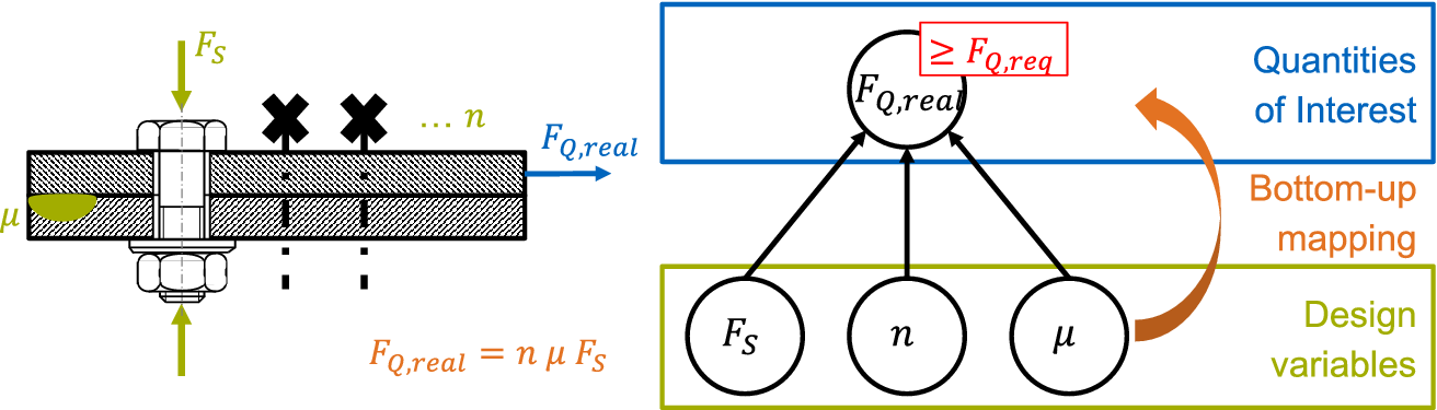
Figure 1. Left: joint design; right: corresponding attribute dependency graph (ADG).
The designer has to determine the number of bolts needed $ n $
and the force applied by
$ n $
and the force applied by $ {F}_S $
. Furthermore, the constant friction coefficient
$ {F}_S $
. Furthermore, the constant friction coefficient $ \mu $
has an influence on the joint. Thus, the relevant attributes are:
$ \mu $
has an influence on the joint. Thus, the relevant attributes are: $ {F}_{Q,\mathrm{real}} $
,
$ {F}_{Q,\mathrm{real}} $
, $ {F}_S $
,
$ {F}_S $
, $ n $
, and
$ n $
, and $ \mu $
. To identify the dependency structure within the attributes, the designer can change the values of all attributes systematically.
$ \mu $
. To identify the dependency structure within the attributes, the designer can change the values of all attributes systematically.
For the application of ADGs, the focus is on the actual behaviour of the system. Desired behaviour and requirements are not considered yet.
-
• $ {F}_S $
: Does a change on
$ {F}_S $
influence the number of bolts
$ n $
? No, the number of bolts can be chosen independently of the force that is applied to them, and vice versa. Does a change on
$ {F}_S $
influence the constant friction coefficient
$ \mu $
? Possibly. For the beginning, we assume that for our design task, the constant friction coefficient is only dependent on the selected materials. Thus, there is no influence between
$ {F}_S $
and
$ \mu $
, as
$ \mu $
also does not have any influence on the applied force. Does a change on
$ {F}_S $
lead to a change in
$ {F}_{Q,\mathrm{real}} $
? Yes.
$ {F}_S $
: Does a change on
$ {F}_S $
influence the number of bolts
$ n $
? No, the number of bolts can be chosen independently of the force that is applied to them, and vice versa. Does a change on
$ {F}_S $
influence the constant friction coefficient
$ \mu $
? Possibly. For the beginning, we assume that for our design task, the constant friction coefficient is only dependent on the selected materials. Thus, there is no influence between
$ {F}_S $
and
$ \mu $
, as
$ \mu $
also does not have any influence on the applied force. Does a change on
$ {F}_S $
lead to a change in
$ {F}_{Q,\mathrm{real}} $
? Yes. -
•
$ n $
: We have already figured out that
$ n $
has no influence on
$ {F}_S $
and
$ \mu $
, but it has an influence on
$ {F}_{Q,\mathrm{real}} $
. -
•
$ \mu $
:
$ \mu $
has no influence on the number of bolts
$ n $
and the applied force
$ {F}_S $
. It also determines
$ {F}_{Q,\mathrm{real}} $
. -
•
$ {F}_{Q,\mathrm{real}} $
:
$ {F}_{Q,\mathrm{real}} $
has no influence on
$ {F}_S $
, as it is a consequence of
$ {F}_S $
. The same applies to
$ \mu $
and
$ n $
. Thus, we cannot control
$ {F}_{Q,\mathrm{real}} $
directly.


We identify $ {F}_S $
,
$ {F}_S $
, $ n $
, and
$ n $
, and $ \mu $
as independently controllable design variables and
$ \mu $
as independently controllable design variables and $ {F}_{Q,\mathrm{real}} $
as an indirectly controllable quantity of interest. Figure 1 (right) shows the corresponding ADG.
$ {F}_{Q,\mathrm{real}} $
as an indirectly controllable quantity of interest. Figure 1 (right) shows the corresponding ADG.
The lower level comprises the design variables, which are independent of each other. $ {F}_{Q,\mathrm{real}} $
constitutes the upper level of quantities of interests (QoIs).
$ {F}_{Q,\mathrm{real}} $
constitutes the upper level of quantities of interests (QoIs).
The bottom-up mapping maps the design variables ( $ n $
,
$ n $
, $ \mu $
and
$ \mu $
and $ {F}_S $
) onto the QoI (
$ {F}_S $
) onto the QoI ( $ {F}_{Q,\mathrm{real}} $
) and can be cast into the form
$ {F}_{Q,\mathrm{real}} $
) and can be cast into the form $ \mathbf{y}=f\left(\mathbf{x}\right) $
, in which
$ \mathbf{y}=f\left(\mathbf{x}\right) $
, in which $ \mathbf{y} $
are QoIs and
$ \mathbf{y} $
are QoIs and $ \mathbf{x} $
are the design variables. For this example, the following formula applies:
$ \mathbf{x} $
are the design variables. For this example, the following formula applies:
 $$ {F}_{Q,\mathrm{real}}=n\hskip0.1em \mu \hskip0.1em {F}_S. $$
With a quantitative model available, the designer is able to check whether or not a design fulfils the requirements of the system, that is, $ {F}_{Q,\mathrm{real}\hskip0.35em }\ge \hskip0.35em {F}_{Q,\mathrm{req}} $
. We do not derive the design from the requirements in the first place, but start with the actual behaviour and then check whether different sets of designs meet the requirements. The designer can now consider all possible designs that fulfil the requirements and not only one design which is derived directly from requirements using assumptions on unknown quantities. This allows for an assumption-free modelling of the system behaviour and design.
$ {F}_{Q,\mathrm{real}\hskip0.35em }\ge \hskip0.35em {F}_{Q,\mathrm{req}} $
. We do not derive the design from the requirements in the first place, but start with the actual behaviour and then check whether different sets of designs meet the requirements. The designer can now consider all possible designs that fulfil the requirements and not only one design which is derived directly from requirements using assumptions on unknown quantities. This allows for an assumption-free modelling of the system behaviour and design.
As ADGs may be adapted to specific design tasks, they may differ for different scenarios of a joint design. Let us assume three independent scenarios:
-
a) The material combination of the two plates is already fixed in the design process. The designer has the freedom to specify the number of bolts
$ n $
and the force
$ {F}_S $
which is applied to them. -
b) In addition to the number of bolts
$ n $
and the applied force
$ {F}_S $
, the designer can choose the materials used for the joint or add additional material between the plates. The designer can thus adjust the friction coefficient, here assumed as constant
$ \mu $
. -
c) Investigations in the R&D department revealed that
$ \mu $
is not constant for the chosen materials, but depends on the applied horizontal force
$ F={F}_S\;n $
. In this case,
$ F $
determines both
$ {F}_{Q,\mathrm{real}} $
and
$ \mu $
.


3.2. Solving the design problems
A designer could start with the required force $ {F}_{Q,\mathrm{req}}=10\;\mathrm{kN} $
. They may assume that four bolts are needed. Furthermore, the designer assumes that the sheets are made of steel and have a friction coefficient of 0.2. Having these values allows the designer to calculate the force which needs to be applied on each bolt:
$ {F}_{Q,\mathrm{req}}=10\;\mathrm{kN} $
. They may assume that four bolts are needed. Furthermore, the designer assumes that the sheets are made of steel and have a friction coefficient of 0.2. Having these values allows the designer to calculate the force which needs to be applied on each bolt: $ {F}_S={F}_{Q,\mathrm{req}}\mu\;N=12.5\;\mathrm{kN} $
. When the requirement changes, the designer needs to recalculate the equation. Furthermore, when additional requirements are introduced it becomes more complicated: Which requirement should we use to start the calculation? Then we have to check whether the other requirements are satisfied. In this case, the applied force might be too high for the bolt used. Therefore, a bolt with a higher strength seems to be required. The designer may have forgotten that they based the calculation on assumptions, such as the number of bolts. ADGs enable assumption
-free design because they do not require any assumptions. Furthermore, when the designer calculates the applied force
$ {F}_S={F}_{Q,\mathrm{req}}\mu\;N=12.5\;\mathrm{kN} $
. When the requirement changes, the designer needs to recalculate the equation. Furthermore, when additional requirements are introduced it becomes more complicated: Which requirement should we use to start the calculation? Then we have to check whether the other requirements are satisfied. In this case, the applied force might be too high for the bolt used. Therefore, a bolt with a higher strength seems to be required. The designer may have forgotten that they based the calculation on assumptions, such as the number of bolts. ADGs enable assumption
-free design because they do not require any assumptions. Furthermore, when the designer calculates the applied force $ {F}_S $
from the requirement on
$ {F}_S $
from the requirement on $ {F}_{Q,\mathrm{real}} $
they confuse design variables with requirements on QoIs.
$ {F}_{Q,\mathrm{real}} $
they confuse design variables with requirements on QoIs. $ {F}_{Q,\mathrm{real}} $
cannot be changed and thus is not controllable. The ADG shows what can be controlled: the number of bolts
$ {F}_{Q,\mathrm{real}} $
cannot be changed and thus is not controllable. The ADG shows what can be controlled: the number of bolts $ n $
, the force applied to the bolts
$ n $
, the force applied to the bolts $ {F}_S $
, and the friction coefficient
$ {F}_S $
, and the friction coefficient $ \mu $
. Consequently, the designer could change the number of bolts or the material instead, depending on the scenario.
$ \mu $
. Consequently, the designer could change the number of bolts or the material instead, depending on the scenario.
In order to solve the design problem in an assumption-free way, we use ADGs and compute solution spaces for the design variables we can control (Zimmermann et al. Reference Zimmermann, Königs, Niemeyer, Fender, Zeherbauer, Vitale and Wahle2017). Figure 2 depicts the ADGs for the scenarios described above.

Figure 2. Attribute dependency graphs (ADGs) for three different joint design scenarios: (a) $ \mu $
is considered as a design parameter, that is, its value is fixed; (b)
$ \mu $
is considered as a design parameter, that is, its value is fixed; (b) $ \mu $
is considered as a design variable, that is, its value can be changed; (c)
$ \mu $
is considered as a design variable, that is, its value can be changed; (c) $ \mu $
is considered as force dependent, that is, its values can only be assigned indirectly by the resulting force
$ \mu $
is considered as force dependent, that is, its values can only be assigned indirectly by the resulting force $ F={nF}_S $
and a characteristic curve
$ F={nF}_S $
and a characteristic curve $ \hat{\mu}(F) $
.
$ \hat{\mu}(F) $
.
In Scenario a), $ n $
and
$ n $
and $ {F}_S $
influence
$ {F}_S $
influence $ {F}_{Q,\mathrm{real}} $
.
$ {F}_{Q,\mathrm{real}} $
. $ \mu $
also influences
$ \mu $
also influences $ {F}_{Q,\mathrm{real}} $
, but the designer has no freedom to change it. For the ADG, there are two possibilities: (1) We can omit this attribute or (2) we can sketch it as a design parameter (i.e., we consider it to be not adjustable) with dashed lines to indicate its influence. Figure 3, Scenario a) depicts the solution space and one possible solution to this design problem. In this scenario,
$ {F}_{Q,\mathrm{real}} $
, but the designer has no freedom to change it. For the ADG, there are two possibilities: (1) We can omit this attribute or (2) we can sketch it as a design parameter (i.e., we consider it to be not adjustable) with dashed lines to indicate its influence. Figure 3, Scenario a) depicts the solution space and one possible solution to this design problem. In this scenario, $ \mu $
is a parameter, so the designer cannot change it. In this case, it is
$ \mu $
is a parameter, so the designer cannot change it. In this case, it is $ \mu =0.2 $
.
$ \mu =0.2 $
. $ {F}_S $
and
$ {F}_S $
and $ n $
are design variables, which can be assigned values to obtain a certain system performance, expressed by
$ n $
are design variables, which can be assigned values to obtain a certain system performance, expressed by $ {F}_{Q,\mathrm{real}} $
. By applying a requirement on
$ {F}_{Q,\mathrm{real}} $
. By applying a requirement on $ {F}_{Q,\mathrm{real}} $
, we divide all possible designs in two groups: good designs, which fulfil all requirements (green dots), and the bad designs, which violate a requirement (red dots). The ADG incorporates the idea of solution spaces by revealing how the designer can influence the system behaviour. There is no need to make any assumptions on the design variables, for example, on the number of bolts
$ {F}_{Q,\mathrm{real}} $
, we divide all possible designs in two groups: good designs, which fulfil all requirements (green dots), and the bad designs, which violate a requirement (red dots). The ADG incorporates the idea of solution spaces by revealing how the designer can influence the system behaviour. There is no need to make any assumptions on the design variables, for example, on the number of bolts $ n $
. According to Figure 3, the designer can choose from different designs which fulfil the requirements, for example,
$ n $
. According to Figure 3, the designer can choose from different designs which fulfil the requirements, for example, $ n=6 $
and
$ n=6 $
and $ {F}_S=10\;\mathrm{kN} $
. The intersection of the two dashed lines in Scenario a) indicates this solution. There are other possible solutions, since every green dot indicates a good design. The designer can incorporate other information in their decision, such as geometrical constraints. Accordingly, the designer wants to use the minimum number of bolts possible (here
$ {F}_S=10\;\mathrm{kN} $
. The intersection of the two dashed lines in Scenario a) indicates this solution. There are other possible solutions, since every green dot indicates a good design. The designer can incorporate other information in their decision, such as geometrical constraints. Accordingly, the designer wants to use the minimum number of bolts possible (here $ n=3 $
). Or they could prefer a robust solution and move the design further away from the limit line, for example, to
$ n=3 $
). Or they could prefer a robust solution and move the design further away from the limit line, for example, to $ n=10 $
or
$ n=10 $
or $ {F}_S=15\;\mathrm{kN} $
.
$ {F}_S=15\;\mathrm{kN} $
.

Figure 3. Solution spaces for three different joint design scenarios. Green dots indicate good designs. Black frames indicate regions of permissible variation.
In Scenario b) the designer can additionally adjust the friction coefficient $ \mu $
. Therefore, it is marked as a design variable. Figure 3, Scenario b) shows the solution spaces for this design task. As we have three design variables, we need two diagrams to depict them. The boundaries of the good design space become blurry because a three-dimensional design space is projected onto two dimensions. We can derive intervals for design variables, which contain only good designs. The rectangular solution spaces depict those intervals. The designer can choose independently one value for each design variable within its intervals.Footnote
4 In this scenario, the designer could also change
$ \mu $
. Therefore, it is marked as a design variable. Figure 3, Scenario b) shows the solution spaces for this design task. As we have three design variables, we need two diagrams to depict them. The boundaries of the good design space become blurry because a three-dimensional design space is projected onto two dimensions. We can derive intervals for design variables, which contain only good designs. The rectangular solution spaces depict those intervals. The designer can choose independently one value for each design variable within its intervals.Footnote
4 In this scenario, the designer could also change $ \mu $
to higher values to get a higher value for
$ \mu $
to higher values to get a higher value for $ {F}_{Q,\mathrm{real}} $
.
$ {F}_{Q,\mathrm{real}} $
.
In Scenario c) we can observe two differences: First, $ {F}_S $
and
$ {F}_S $
and $ n $
influence
$ n $
influence $ {F}_{Q,\mathrm{real}} $
directly and indirectly via
$ {F}_{Q,\mathrm{real}} $
directly and indirectly via $ F $
and
$ F $
and $ \mu $
. Indirect dependencies make the behaviour of complex systems less intuitive. ADGs can model this influence in a unique way without circular dependencies. Second, the characteristic curve
$ \mu $
. Indirect dependencies make the behaviour of complex systems less intuitive. ADGs can model this influence in a unique way without circular dependencies. Second, the characteristic curve $ \hat{\mu}(F) $
is an attribute.
$ \hat{\mu}(F) $
is an attribute. $ \hat{\mu}(F) $
characterises the behaviour of the material. The realised friction coefficient depends on the force
$ \hat{\mu}(F) $
characterises the behaviour of the material. The realised friction coefficient depends on the force $ F $
. As
$ F $
. As $ {F}_S $
and
$ {F}_S $
and $ n $
are design variables, we do not know a priori what value the friction coefficient
$ n $
are design variables, we do not know a priori what value the friction coefficient $ \mu $
will have. As soon as we assign
$ \mu $
will have. As soon as we assign $ {F}_S $
and
$ {F}_S $
and $ n $
values, we can calculate the specific friction coefficient for a specific force
$ n $
values, we can calculate the specific friction coefficient for a specific force $ F=n\;{F}_S $
with the characteristic curve. In this design scenario, the characteristic curve itself is considered as fixed. Therefore, it is handled as a design parameter. In this case, we again only have two design variables, as
$ F=n\;{F}_S $
with the characteristic curve. In this design scenario, the characteristic curve itself is considered as fixed. Therefore, it is handled as a design parameter. In this case, we again only have two design variables, as $ \mu $
is determined by
$ \mu $
is determined by $ {F}_S $
,
$ {F}_S $
, $ n $
, and
$ n $
, and $ \hat{\mu}(F) $
. Figure 3, Scenario c) shows the corresponding solution space with possible intervals for the design variable values. We can see that the limit curve differs from Scenario a). In Scenario a),
$ \hat{\mu}(F) $
. Figure 3, Scenario c) shows the corresponding solution space with possible intervals for the design variable values. We can see that the limit curve differs from Scenario a). In Scenario a), $ \mu =0.2 $
is fixed. In Scenario c), its value depends on
$ \mu =0.2 $
is fixed. In Scenario c), its value depends on $ {F}_S $
and
$ {F}_S $
and $ n $
. The different shapes of the good design space visualise that indirect influence.
$ n $
. The different shapes of the good design space visualise that indirect influence.
For all three design tasks, ADGs show which attributes the designer can influence and how they interact with each other. ADGs can also depict indirect dependencies and characteristic curves without circular dependencies. They pave the way for an assumption-free quantitative design, as can be seen in this example for SSE.
4. The method
4.1. When to apply this method
ADGs can help engineers in the decomposition of complex technical systems (such as a production printer) in collaborative design processes. A system engineer’s task might be to break down overall system objectives (e.g., image quality, productivity and cost) to multiple subsystems (e.g., print head, transportation system and drying unit) and to ensure the successful interaction of the subsystems to achieve the system objectives. In this task, the ADG helps to identify the dependencies between subsystems and to investigate conflicting system objectives (e.g., image quality versus cost). Early in the design phase, the system engineer might only draw an abstract ADG. During the course of the project, the ADG can be detailed to design variables of the identified necessary components.
System engineers can use ADGs for systems design. They are built for a design problem in a specific context. Typically, systems are to be designed such that they fulfil certain requirements. To design systems, the values of design variables have to be determined. By interaction according to physical laws, all attributes generate a system behaviour, which then either fulfils the given requirements or not.
ADGs show which attributes interact with each other to generate a certain system behaviour. ADGs do not necessarily require quantitative models of the dependencies, for example, by formulae. However, quantitative models can help to set up the dependency structure, as the formula did in the introductory example. ADGs can be used in SSE (Zimmermann et al. Reference Zimmermann, Königs, Niemeyer, Fender, Zeherbauer, Vitale and Wahle2017) to describe the system that needs to be modelled.
We regard design as an activity to choose values for the controllable attributes (design variables) in a way that fulfils the requirements attached to noncontrollable attributes (quantities of interest).
An ADG documents the quantities that are used to formulate INUS conditions. Mackie (Reference Mackie1965) defines an INUS condition as an insufficient but necessary part of an unnecessary but sufficient condition for an effect to occur. In this sense, INUS conditions may be called a cause for a certain effect. In the joint design example above, we have three causes for the effect that the plate can support a certain horizontal force $ {F}_Q $
: the number of bolts
$ {F}_Q $
: the number of bolts $ n $
; the force applied by the bolts
$ n $
; the force applied by the bolts $ {F}_S $
; and the friction coefficient
$ {F}_S $
; and the friction coefficient $ \mu $
. Satisfying a requirement on one of these quantities is insufficient: One or several bolts alone, without any force applied and without any friction coefficient, do not support a lateral force. A force which cannot be applied does not help either. A friction coefficient alone, without any vertical force, cannot support a horizontal force. At the same time, satisfying each requirement associated with one of the quantities is necessary: If we do not use one bolt we cannot apply a force. If we do not apply a force, a lateral horizontal force cannot be supported. The same applies to the friction coefficient. Satisfying all requirements on them is sufficient for the desired effect to occur, that is, to support a horizontal force. But this set is not necessary. Other sets of INUS conditions can support a horizontal force: The plate can be so heavy that it provides enough vertical force, so no bolts are needed. The plates could be welded together, so that the set consisting of bolts, vertical force, and friction coefficient would not be necessary. They would then constitute different designs and be described by different ADGs.
$ \mu $
. Satisfying a requirement on one of these quantities is insufficient: One or several bolts alone, without any force applied and without any friction coefficient, do not support a lateral force. A force which cannot be applied does not help either. A friction coefficient alone, without any vertical force, cannot support a horizontal force. At the same time, satisfying each requirement associated with one of the quantities is necessary: If we do not use one bolt we cannot apply a force. If we do not apply a force, a lateral horizontal force cannot be supported. The same applies to the friction coefficient. Satisfying all requirements on them is sufficient for the desired effect to occur, that is, to support a horizontal force. But this set is not necessary. Other sets of INUS conditions can support a horizontal force: The plate can be so heavy that it provides enough vertical force, so no bolts are needed. The plates could be welded together, so that the set consisting of bolts, vertical force, and friction coefficient would not be necessary. They would then constitute different designs and be described by different ADGs.
4.2. Classification in graph theory
According to the classification in graph theory developed by Diestel (Reference Diestel2006) as summarised in Kreimeyer (Reference Kreimeyer2009), an ADG has the following properties:
-
• It is a directed graph (‘digraph’), as it contains only directed edges and nodes.
-
• Neither nodes nor edges have (per se) weights (‘nonweighted graph’).
-
• Is is a ‘simple graph’, as no node can have an edge with itself (loops).
-
• ‘Hyperedges’ are allowed (one edge connecting one node to many others), but it is not a ‘multigraph’, as between two nodes there can only be one edge or none.
-
• ‘Half-edges’ or ‘loose edges’ are not part of it, as every edge has to connect two nodes.
-
• Similarly, no ‘disconnected’ nodes are admitted.
-
• It is a ‘node-labelled graph’ because every node contains a label, while edges do not.
-
• ‘Complete’ graphs or ‘cliques’, where every node is connected to every other node, are not possible in ADGs, as nodes on the same hierarchical level cannot be connected to each other.
-
• An ADG is a polyhierarchy because a source node can have multiple dependent nodes.Footnote 5
4.3. Terms and definitions
Nodes represent attributes. There are three types of attributes (aligned with Papalambros & Wilde Reference Papalambros and Wilde2017):
-
• Design variables (DVs): The attributes that have to be defined during the design process. They are controllable and thus constitute operating levers for the designer. Characteristics, such as
$ \hat{\mu}(F) $
, are also considered to be design variables. -
• Design parameters (DPs): In most design processes there are attributes that could be changed, but are assumed as fixed due to restrictions or decisions (e.g., modulus of elasticity after deciding for a specific material).
-
• Quantities of interest (QoIs): The attributes at the highest level of the ADG. They cannot be controlled directly. QoIs describe the behaviour of a system. Requirements on the QoIs can be used to formulate the design goal.

In addition to attributes, there are also constants that cannot be changed and are not the focus of the design process. Usually, they are not depicted. They could be added in the same way design parameters are added, if helpful for understanding. The design attributes (variables and parameters) are found on the bottom layer of the graph. They have no input but have one or several outputs. When the scope of the ADG changes, the role of the attributes in the graph may change. The DVs of an ADG on a system level may become the QoIs of an ADG on the component level. In the course of the design processes, attributes can also change their role, depending on the element in focus. What is a QoI for one person (output of their design task) can be an input for somebody else’s design task.
Within the hierarchy of the ADG, there are also nodes between design variables and QoIs – we call them intermediate attributes. They always have both, inputs and outputs. All edges in the ADG represent dependencies. They are directed from a lower to a higher level (bottom-up).
Note that two elements on the same level of the hierarchy can never influence each other, but together they can influence elements on higher levels (if they are both linked to it). In the terminology of this article that means there is never a (direct) dependency between two elements on the same level of hierarchy.
The term dependency in this case is (part of) the relation between a controllable attribute (design variable) and noncontrollable attribute in the sense of a system response. ADGs do not represent an intended behaviour, but rather an expected or emerging behaviour. We see the system response as the behaviour of a product as a result of a design choice. The system response is the consequence of a specific design, that is, assigning specific values to design variables. System behaviour in this context does not mean a time-dependent behaviour, like we can observe it in dynamic simulations, for example. We can use dynamic simulations to quantify QoIs (e.g., maximum acceleration values), but the quantity of interest itself is not time-dependent because it describes the performance of the product. Furthermore, we can use time-dependent characteristic curves (e.g., for damping in an oscillating system) as attributes to model the system behaviour (e.g., the eigenfrequency).
Along that path between a design variable on the lowest level of the ADG and the respective QoI at the top, cuts can be made in any position, similar to free body diagrams in mechanics.
The rules depicted in Figure 4 give guidance for modelling ADGs. The attributes of the ADG have to be arranged so that the attributes on the lower level have their values assigned first. The values of the superordinate attributes follow as the result (emerging behaviour) and are only controlled by the attributes on the lower levels. If we want to model the dependency of power, mass, and acceleration of a vehicle, we would first assign values to the mass and the power, so those attributes would belong on the lower level of the graph. In addition, we can set values for mass (chassis) and power (engine) independently. Only by combining the values for mass and power can we determine the acceleration of the overall product (vehicle). It is possible that an attribute Z is directly dependent on an attribute Y and at the same time has one or more indirect dependencies from Y.

Figure 4. Rules and guidelines for modelling an ADG (scheme oriented on Lindemann, Maurer & Braun Reference Lindemann, Maurer and Braun2008).
In software engineering, research indicates that circular dependencies have an impact on the proneness of changes (Oyetoyan et al. Reference Oyetoyan, Falleri, Dietrich and Jezek2015). Circular dependencies occur when two or more software blocks mutually depend on each other. That means, for example, that block A needs the result from block B but block B needs the result from block A. If there is no termination condition, the circular dependency results in infinite loops. In ADGs, dependencies must always point from bottom to top. They cannot point backwards. Therefore, circular dependencies are by definition excluded.
To make the ADG easier to read, multiple dependencies can be grouped and joined into one edge. The above attribute is then dependent on all attributes connected. Design parameters can be displayed or left out of an ADG. When included, we mark them with a dotted circle to differentiate them from design variables. We distinguish between requirements and attributes. Requirements can be displayed in a rectangle attached to the attribute it refers to. Requirements are mostly found on the upper level, as requirements formulated for the QoIs of the system. Nevertheless, requirements can be also formulated for intermediate attributes or design variables. For the latter, they impose limits on the design space.
In the case of building a quantitative model from the ADG, a further aspect should be considered: Generally, an attribute is a physical quantity (e.g., mass) or a characteristic (e.g., battery voltage over state of charge). However, for a quantitative model, all attributes or characteristics need to be measurable. That might not be the case for tastes or feelings (e.g., familiarity as a response to a product design).
4.4. Procedure model for building ADGs
Engineers who trained their causal thinking in the way described above can build simple ADGs intuitively. For beginners or more complex systems, we suggest using the following procedure to build ADGs (see Figure 5):
-
1. Define the system of interest and its boundaries. Collect components and subsystems of the product.
-
2. Collect attributes that describe the behaviour/performance of the system. For this step, requirements or attributes communicated to customers can be a source for QoIs. In product development, requirements on these attributes can lead to conflicts of goals during the design process (e.g., mass and strength).
-
3. Collect attributes which (a) describe the subsystems and components, (b) influence the system behaviour, or (c) need to be assigned values during the design process.
-
4. Group controllable (design variables; bottom) and noncontrollable attributes (QoIs; top). The remaining attributes stay in between as intermediate attributes.
-
5. Determine dependencies using formula or expert knowledge and draw edges from the bottom to the top until all attributes are connected with at least one edge. Think of which attributes can be assigned values first and which values emerge after those values are set. Do not confuse them with requirements. We are not looking at required or desired behaviour yet, but only at the emerging behaviour of the system.

Figure 5. Procedure model for building attribute dependency graphs.
This is one proposed procedure. Others are possible. Sometimes an ADG has to be amended when new information is available. Thus, the procedure is iterative as indicated by the dotted triangles pointing upwards in Figure 5. To verify sections of the ADG during the process, it is helpful to translate those sections into a quantitative model and to use SSE to visualise the solution space. This visualisation reveals if the dependencies used are plausible and provide meaningful results. This may lead to an iterative process of adapting the ADG and the quantitative model until both reach a satisfactory level.
5. Examples
We present two further examples of ADGs in design projects: (1) garden hose box design and (2) vehicle dynamics design.
5.1. Garden hose box design
Figure 7 displays two ADGs of a garden hose box as shown in Figure 6. The upper ADG shows the abstracted dependencies of the hose box while the lower ADG is a zoom into the upper ADG and therefore reveals more detail. The example shows that it is possible to zoom in and out of ADGs to allow examination at different levels of detail. The abstracted ADG helps to obtain an initial understanding about considered components, QoIs and their dependencies. The detailed ADG specifies the variables actually used to model the components. The latter is needed to effectively support the design task described in the following.

Figure 6. Sketch and section of the hose box. The quantities are explained in Figure 7.

Figure 7. Abstracted and detailed ADG of the hose box (zoomed in and out).
The ADG of the hose box was used in a design project presented by Rötzer et al. Reference Rötzer, Thoma and Zimmermann2020b. One of the key questions in this project was to determine if sharing components among different product variants is technically feasible and economically beneficial.
The hose box serves the functions of containing, dispensing, and retracting a predefined garden hose. The box consists of three cost-driving components: housing, reel and spring. To reduce the complexity, the model of the hose box uses a fixed layout of the components. That means, for example, that different installation positions for the spring are not considered. Furthermore, the model includes only those attributes of the components that are necessary to evaluate if components can and should be shared among products (different variants offered to the customer). Ten design variables describe the geometry of the components (see Figures 6 and 7). The ADG does not show design parameters (attributes that are considered unchangeable for the analysis), such as the wall thickness of the spool and housing or the diameter of the water hose. On the top level, the ADG shows 10 QoIs of the system. Out of those, the hose length ( $ {l}_{\mathrm{Hose}} $
) and the aspect ratio of the housing (
$ {l}_{\mathrm{Hose}} $
) and the aspect ratio of the housing ( $ {r}_{\mathrm{Housing}} $
) are used to measure the fulfilment of customer requirements. The other QoIs are mainly needed to guarantee the technical feasibility of the hose box design (e.g., (
$ {r}_{\mathrm{Housing}} $
) are used to measure the fulfilment of customer requirements. The other QoIs are mainly needed to guarantee the technical feasibility of the hose box design (e.g., ( $ {r}_{d,\mathrm{hose}} $
) guarantees that the reel’s diameter is large enough to ensure a sufficient bending curve for the hose).
$ {r}_{d,\mathrm{hose}} $
) guarantees that the reel’s diameter is large enough to ensure a sufficient bending curve for the hose).
Most QoIs depend on multiple design variables. Intermediate attributes in the ADG can help to structure the dependencies between QoIs and DVs. An example illustrates this: The spring variables have an influence on multiple QoI. However, the influence is not attributed to a single design variable of the spring, but rather the interaction of the five spring design variables. Therefore, the spring characteristic $ {C}_S $
, as an intermediate attribute, helps to structure the ADG. The spring characteristic describes the torque curve over the revolutions of the spring. This demonstrates that ADGs can represent whole characteristic curves and not only numerical variables. When translating the ADG into a quantitative model, characteristic grid points of the curve are used as an approximation for the curve.
$ {C}_S $
, as an intermediate attribute, helps to structure the ADG. The spring characteristic describes the torque curve over the revolutions of the spring. This demonstrates that ADGs can represent whole characteristic curves and not only numerical variables. When translating the ADG into a quantitative model, characteristic grid points of the curve are used as an approximation for the curve.
It might be assumed that the size of the spring has an influence on the size of the reel, and that the size of the reel influences the size of the housing. But in ADGs there are no direct dependencies between the design variables (in this case, the geometrical attributes of housing, reel and spring). However, when looking at the hose box as a combined system of the aforementioned components, the geometrical attributes of the components together influence the QoI of the system, that is, there must be a gap between the components. Or to put it differently, the components may not overlap. The ADG helps to solve these indirect dependencies without directly deriving one component from another. We only verify if the requirement of leaving a gap between the components is fulfilled. The components can be examined independently. This independence of the components means that they can be examined individually for standardisation potential.
The ADG supported the process of creating a shared understanding of the system and its necessary relationships among the project participants in an early phase. In an iterative process, the ADG was adapted and discussed in order to arrive at the most accurate representation of the system possible.
The numerical optimization of the product family of hose boxes required a quantitative model of the hose box in program code. The ADG helped to figure out the dependencies for which quantitative models had to be found. That is why we see the ADG as a support for quantitative modelling. Moreover, the ADG serves as a checklist during the implementation of the mathematical model, where every dependency (edge) of the graph needs to be translated to a function of the mathematical model. For the hose box, the ADG helped to determine the attributes for an artificial neural network (ANN, see Figure 7) and to systematically look for a spring design tool which can calculate the characteristic curve of the spring ( $ {C}_S $
) from the geometrical attributes (
$ {C}_S $
) from the geometrical attributes ( $ {d}_{\mathrm{Spring}} $
,
$ {d}_{\mathrm{Spring}} $
, $ {d}_{\mathrm{Arbor}} $
,
$ {d}_{\mathrm{Arbor}} $
, $ {w}_{\mathrm{Coil}} $
,
$ {w}_{\mathrm{Coil}} $
, $ {t}_{\mathrm{Coil}} $
,
$ {t}_{\mathrm{Coil}} $
, $ {l}_{\mathrm{Coil}} $
). This was necessary because no formula was available to calculate the characteristic of this specific kind of power spring. The ADG helped to identify and specify the missing piece of the overall quantitative model in order to efficiently create a suitable surrogate model. After the quantitative model was finished, the ADG helped to explain both the system and the quantitative model to new stakeholders. Therefore, we recommend keeping the quantitative model and the ADG synchronised.
$ {l}_{\mathrm{Coil}} $
). This was necessary because no formula was available to calculate the characteristic of this specific kind of power spring. The ADG helped to identify and specify the missing piece of the overall quantitative model in order to efficiently create a suitable surrogate model. After the quantitative model was finished, the ADG helped to explain both the system and the quantitative model to new stakeholders. Therefore, we recommend keeping the quantitative model and the ADG synchronised.
Now, consider a scenario in which we design the hose box without the use of ADGs. We might begin by designing the spool or the spring according to the requirements. If we start with the spool, we have to design a spool that can accommodate the required hose (specified by length and diameter). Then, we might design a spring that facilitates the retraction of the hose according to the chosen spool. At that point, we might notice that it is impossible to find a spring that fits into the reel’s diameter while yielding sufficient turns and torque for retraction. We then go one step back and choose a spool design with a greater diameter. By increasing the outer diameter of the spool, the number of vertical hose layers can be increased. In order to keep the total box dimensions low, as a next step, the horizontal layers, and therefore the width of the spool, can be decreased. However, by using more vertical layers, the lever for retraction force increases, requiring a higher momentum from the spring. This may result in the need for a larger spring again. The designer might get stuck in a circle of increasing both reel and spring. By jumping back and forth from the QoIs to the DVs, this traditional approach can lead to unnecessary effort in the design process. The ADG a priori eliminates circular dependencies by breaking down the requirements on the QoIs to the DVs. That allows us to determine designs that simultaneously fulfil all requirements without unnecessary loops during the design process.
5.2. Vehicle dynamics design
Figure 8 shows the ADG for an industry project on vehicle dynamics design. Due to nondisclosure reasons, some of the content is redacted. This example illustrates how an ADG helps to structure and organise many dependencies of a complex system. It is structured according to the abstraction levels of the V-model: it starts from customer-related attributes on the top level and ends with the attributes of components on the bottom level. For better visualisation, a zoomed-out ADG is shown. The grey boxes contain groups of attributes which belong to a certain cluster, such as axle bearings containing different bearing stiffnesses (component level) or cornering characteristics containing eigenfrequencies and max. lateral accelerations (vehicle (subjective) level). This was done to provide a better overview than a fully expanded ADG with all attributes and dependencies visualised. The detailed information does not get lost and the overall dependencies are still valid. If users want a detailed view, they can zoom in and expand the grey boxes to ADGs themselves.

Figure 8. Attribute dependency graph (ADG) for vehicle dynamics design; top: assignment of attributes to components; bottom: assignment of attributes to quantitative models.
On the top of Figure 8, we can also see that the designers have highlighted some clusters of attributes to indicate their affiliation to a specific system, such as suspension. Additional disciplines, such as durability, acoustics or crash, can connect their ADGs with this ADG. It can be easily extended. Further attributes can be added horizontally. The user then simply has to check whether existing attributes contribute to the attributes added. It does not change the existing dependencies. Describing the components in a more detailed way extends the ADG vertically – we can go from designing subsystems to designing components. Existing DVs might then turn into intermediate attributes as new DVs are introduced, but the interactions of the existing attributes in the system are preserved. This supports a holistic view and thus an overall understanding of the system. In this example, many engineers collaborate to design this complex system. ADGs can help to systematically store knowledge about dependencies within a department and share it with other departments. The clear rules of an ADG can serve as a common language for different designers. Consequently, it can enable interdisciplinarity in complex system design.
The bottom of Figure 8 shows examples of how designers use different quantitative models to quantify the dependencies in the ADG: multibody dynamic simulations, a formula-based 2-track model, or a response surface approximation as a surrogate model. Even the driver can be modelled according to this logic if the necessary data is available. Furthermore, missing models can be identified easily. The ADG lists all attributes which need to be modelled. This supports quantitative system design. Missing models can be identified, as every edge needs to be expressed by a model. Furthermore, complex dependencies from the bottom to the top can be traced and visualised. This helps designers to identify how a change on the component level can influence the system level. This can provide transparency during the design of a complex system.
6. Discussion, summary and outlook
6.1. Discussion
This section discusses the limitations of ADGs, the modelling of cyclic dependencies, and the characteristics of ADGs.
Limitations
ADGs have limitations similar to many other modelling techniques in technical product development, without tool support it is difficult to handle large amounts of information. This is especially crucial for large ADGs of complex systems. They can become confusing due to the high number of nodes and edges crossing each other. Ideally, the tool used has the following features: (a) automatic graph creation based on input data (e.g., adjacency matrix), (b) path visualisation: highlighting all attributes which are connected to a selected attribute, (c) automatic reordering of attributes such that intersections between edges are minimised and, (d) capability to zoom in and out (grouping nodes and edges in black boxes).
Unless the designers applying this method have the necessary in-depth education and training, models cannot practically fulfil their purposes of providing an explanation and overview (Tomiyama et al. Reference Tomiyama, van Beek, Cabrera, Komoto and D’Amelio2013). Designers need to learn and understand the rules of an ADG before applying them. This obstacle may hinder its application.
ADGs require an understanding of the system at hand. Users need to understand the underlying physical effects in order to model the dependencies correctly. It does not provide a framework to check whether or not drawn links are correct. This can lead to ADGs that do not comply with the rules or have incorrect cause-and-effect chains. For the most part, formulas or simulation provide sufficient knowledge, but in some instances, empirical data from tests might be needed. In this case, the methodology developed by Pearl & Mackenzie (Reference Pearl and Mackenzie2019) might be useful. It uses stochastic methods to determine whether there are causal dependencies between attributes. It may also provide formulas to describe the effect quantitatively.
ADGs provide a clear causal framework to visualise dependencies for complex system design. The fact that circular dependencies are excluded by definition can help to avoid unintended iterations during the design process that can arise when engineers start the process with requirement values. They derive a point-based design which fulfils exactly the requirement. However, technical products usually need to fulfil many requirements from different disciplines. It is likely that this point-based design does not fulfil all other requirements of the product. Designers thus iterate until they find a point which fulfils all requirements. This process consumes development time. ADGs can help to escape that vicious circle of unintended iterations by clearly distinguishing between emerging and desired behaviour. The ADG itself illustrates emerging behaviour. Requirements applied to certain attributes, usually to the QoIs, represent desired behaviour. ADGs in conjunction with SSE can help to find areas of good designs (set-based design) subject to conflicting goals (Zimmermann et al. Reference Zimmermann, Königs, Niemeyer, Fender, Zeherbauer, Vitale and Wahle2017). However, the combination with SSE only works when attributes and dependencies can be expressed quantitatively.
Cyclic dependencies
Nevertheless, there are coupled problems in complex system design. One may argue that the proposed method cannot model feedback. This is true if we look at the dynamic relations in technical systems. ADGs focus more on design than on dynamic, that is, time-dependent, description of the behaviour. The prey–predator model can illustrate the difference. The Lotka-Volterra equations can describe the model (Lotka Reference Lotka1910). Figure 9 shows two graphical representations of this model. The Index $ 1 $
describes the prey species, index
$ 1 $
describes the prey species, index $ 2 $
the predator species.
$ 2 $
the predator species. $ N $
is the population of a species,
$ N $
is the population of a species, $ {r}_d $
its death and
$ {r}_d $
its death and $ {r}_r $
its reproduction rate. In the time-dependent model (Figure 9, left) both populations are influenced by their death and reproduction rates. Furthermore, both populations influence each other. This can be called feedback.
$ {r}_r $
its reproduction rate. In the time-dependent model (Figure 9, left) both populations are influenced by their death and reproduction rates. Furthermore, both populations influence each other. This can be called feedback.

Figure 9. Prey–predator model according to the Lotka-Volterra equations (Lotka Reference Lotka1910). Left: Dynamic, coupled system behaviour. Right: ADG.
The ADG does not model those kind of feedback loops (see Figure 9, right). It distinguishes between design variables (bottom) and QoIs (top). If we consider the prey–predator problem as a design problem, the mean values of our populations $ {\overline{N}}_1 $
and
$ {\overline{N}}_1 $
and $ {\overline{N}}_2 $
will be interesting, as will be the characteristic curves of each population
$ {\overline{N}}_2 $
will be interesting, as will be the characteristic curves of each population $ {\hat{N}}_1 $
and
$ {\hat{N}}_1 $
and $ {\hat{N}}_2 $
. The coupled system model from the right side will still be used to calculate the characteristic curves for both populations, but the perspective on the problem is different. ADGs can provide further insights, for example, that the average population of each species depends only on the reproduction and mortality rates of the other species and not on its own. According to that model, the designer could increase the death rate of the predators (e.g., through hunting) to increase the mean population of the prey, but it would not help to increase the birth rate of the prey species (e.g., by breeding). ADGs show how a behaviour can be influenced rather than the time-dependent behaviour itself. It simplifies the problem by distinguishing between controllable and uncontrollable attributes. However, ADGs do not model circular dependencies. The model of the time-dependent behaviour is not a focus. This may increase the understanding of the overall system at the expense of less knowledge about the dynamic relations within the system.
$ {\hat{N}}_2 $
. The coupled system model from the right side will still be used to calculate the characteristic curves for both populations, but the perspective on the problem is different. ADGs can provide further insights, for example, that the average population of each species depends only on the reproduction and mortality rates of the other species and not on its own. According to that model, the designer could increase the death rate of the predators (e.g., through hunting) to increase the mean population of the prey, but it would not help to increase the birth rate of the prey species (e.g., by breeding). ADGs show how a behaviour can be influenced rather than the time-dependent behaviour itself. It simplifies the problem by distinguishing between controllable and uncontrollable attributes. However, ADGs do not model circular dependencies. The model of the time-dependent behaviour is not a focus. This may increase the understanding of the overall system at the expense of less knowledge about the dynamic relations within the system.
When modelling dependencies, designers usually do not distinguish between controllable and uncontrollable attributes. They rather say components or attributes influence each other. This general influence can be modelled with design structure matrices (DSMs). The term dependency is typically not defined and often subject to the user’s choice.
In the following example, the connection between ADGs and DSMs will be explained for two components that both influence the system behaviour. A ‘1’ in the DSM means, following Luo (Reference Luo2015), that a change of this component affects the functional performance or the value of the corresponding component, “indicating the requirement for co-redesign or change propagation”. Figure 10 shows the corresponding DSMs of the models from Figure 9.

Figure 10. Design structure matrices based on Figure 9. Left: Dynamic, coupled system behaviour. Right: ADG.
First, we define the components $ C1 $
and
$ C1 $
and $ C2 $
as consisting of all attributes describing the prey and predator species, respectively. The DSM based on the coupled model has only entries with values one, as all components influence each other and are fully coupled.
$ C2 $
as consisting of all attributes describing the prey and predator species, respectively. The DSM based on the coupled model has only entries with values one, as all components influence each other and are fully coupled.
To build a DSM that models an ADG we first set up its DMM. The DMM contains information on how the components are linked to the QoIs. To derive the corresponding DSM we multiply the matrix by its inverse. Now the components are linked with each other via the QoIs. This DSM is also fully coupled. This represents what designers often call dependency. In the language of ADGs, it means two or more components affect the same QoI. So if one component is changed, that is, its design variable values are changed, it may be necessary to change another component as well to get again a certain system behaviour, represented by the QoIs. The numbers in this DSM indicate how many QoIs the components jointly contribute to. For example, components $ C1 $
and
$ C1 $
and $ C2 $
contribute jointly to
$ C2 $
contribute jointly to $ {\hat{N}}_1 $
and
$ {\hat{N}}_1 $
and $ {\hat{N}}_2 $
. Thus, it has the entry ‘2’. So assuming that a component is dependent on another component if both contribute to the same QoI, we can transfer the ADG to the more commonly used DSM and show that ADGs are not limited to systems without circular dependencies. The presented approach does not model dependency cycles that are often considered in change propagation. This requires a change in mindset and makes the creation of an ADG nonintuitive. This is an obstacle in the application of ADGs.
$ {\hat{N}}_2 $
. Thus, it has the entry ‘2’. So assuming that a component is dependent on another component if both contribute to the same QoI, we can transfer the ADG to the more commonly used DSM and show that ADGs are not limited to systems without circular dependencies. The presented approach does not model dependency cycles that are often considered in change propagation. This requires a change in mindset and makes the creation of an ADG nonintuitive. This is an obstacle in the application of ADGs.
In contrast to ADGs, DSMs cause cycles because they do not distinguish between what is realised (bottom-up) and what is required (top-down view in ADG). Similarly, time-dependent input and output signals that can be cyclic, for example, between components of dynamical systems, are not considered in ADGs. Therefore, ADGs model only the result of time-dependent behaviour, however, they do not solve time-dependency explicitly.
Clear rules guide the creation of ADGs. They represent the grammar of a language. Designers can use this language to communicate their ideas and knowledge with each other. In general, designers often have different concepts of dependency in mind, which impedes a common representation of knowledge. The structure and universality of ADGs can serve as a foundation for a knowledge database in companies. Designers can express their knowledge and connect it with those of other designers through ADGs. With this approach, a holistic view of the dependencies is realised step by step, including the experts’ knowledge of the subsystems and components.
Characteristics of ADGs
In the following, we discuss the fulfilment of the requirements described in the introduction. This article shows three applications of ADGs for engineering design problems: joint design, water hose box design and vehicle dynamics design.
ADGs are able to avoid circular dependencies. There are only dependencies allowed from the level of DVs to the level of QoIs. This allows the creation of a dependency structure without circles. However, coupled dependencies exist in complex systems. ADGs do not represent them. This may lead to confusion and necessitates a change in mindset. However, when subsequently quantifying the dependencies coupled models can be used without restrictions. The requirement is fulfilled, but its representation is not always intuitive. This makes it difficult for new users to apply the method.
ADGs can offer a clear cause and effect structure. The flow of information is bottom-up and the graph is a polyhierarchy. Accordingly, the connections between causes at the bottom and effects to occur at the top are explicit. It helps the designer to better understand the degrees of freedom, that is, which attributes can be controlled. It also fosters an understanding of which attributes a change will affect. However, building this structure according to the rules requires training. Otherwise, the user will not be able to build an ADG. Although ADGs should be unique, sometimes there may be more than one solution to a problem, for example, in the case of tolerance chains. In tolerance chains, it is difficult to determine which length is there ‘first’ and which one influences the other. For problems like this, the ADG cannot provide a clear cause and effect structure and is subject to interpretation.
ADGs should not only provide a clear structure but also support quantitative modelling. Due to the unique bottom-up structure, quantitative models can be made of the form $ y=f(x) $
, where
$ y=f(x) $
, where $ x $
are the attributes on a lower level and
$ x $
are the attributes on a lower level and $ y $
the ones on a higher level. It can contain physical attributes and thus represent a physical model, which helps to build quantitative models upon ADGs and vice versa. This is especially helpful when the quantitative model is not known a priori. ADGs provide a perfect basis for neural networks. The user can directly identify the attributes a neural network needs to fill the gap in the overall system model. The user can plan suitable simulations or experiments efficiently. On the other hand, knowledge about the system at hand is necessary. A user without sufficient knowledge of the (technical) dependencies of the system cannot build an ADG. If a quantitative model is already available, using an ADG can help to explain the scope, setup, and used attributes to people who are not familiar with the model. This can simplify collaboration and knowledge sharing. Note that there are no restrictions on the type of bottom-up mappings: They can be high-dimensional and nonlinear. They only need to have a required input and output.
$ y $
the ones on a higher level. It can contain physical attributes and thus represent a physical model, which helps to build quantitative models upon ADGs and vice versa. This is especially helpful when the quantitative model is not known a priori. ADGs provide a perfect basis for neural networks. The user can directly identify the attributes a neural network needs to fill the gap in the overall system model. The user can plan suitable simulations or experiments efficiently. On the other hand, knowledge about the system at hand is necessary. A user without sufficient knowledge of the (technical) dependencies of the system cannot build an ADG. If a quantitative model is already available, using an ADG can help to explain the scope, setup, and used attributes to people who are not familiar with the model. This can simplify collaboration and knowledge sharing. Note that there are no restrictions on the type of bottom-up mappings: They can be high-dimensional and nonlinear. They only need to have a required input and output.
With this structure, ADGs also enable SSE, which requires a circular-free and unique bottom-up mapping (Zimmermann et al. Reference Zimmermann, Königs, Niemeyer, Fender, Zeherbauer, Vitale and Wahle2017). The ADG visualises which design attributes the user can use to change the system behaviour. With the application of SSE, a user does not need to make any assumptions. All design variables are varied simultaneously and the set of good designs, which fulfil all requirements, is calculated.
These so-called solution spaces break down requirements from a system to a component level. Zimmermann et al. (Reference Zimmermann, Königs, Niemeyer, Fender, Zeherbauer, Vitale and Wahle2017) focus on the calculation of these solution spaces based on simulations. Several publications elaborate on that (see Section 2.2). However, there is no publication yet, which describes the dependency structure which is the basis for the solution space approach. This cause and effect-based dependency modelling is often not intuitive and challenging for users. Zimmermann et al. (Reference Zimmermann, Königs, Niemeyer, Fender, Zeherbauer, Vitale and Wahle2017) provide no explanations, rules or guidelines on how to model those dependencies. They are an essential contribution of this article.
A user can zoom in and out without losing information. This helps to discuss and communicate the design problem for different levels of complexity. ADGs can be abstracted or even collapsed to the attributes themselves. The overall dependency structure is obtained but is no longer displayed in such detail. In order to maintain all information when zooming out, adequate tool support is needed. Otherwise, a user must create separate ADGs and the benefit of zooming in and out is marginalised. To date, there is no such software available for free. This also hinders a wide application of the method. Furthermore, symbols often describe the nodes. This makes the use of a legend necessary for more complex systems, since some users may not know the meaning of the symbols. When grouping parts of an ADG together, the user has to give names to the new nodes. This requires an action on the user’s side.
Different users can extend ADGs. They can add new components and subsystems by adding their attributes and connect them to the existing ones. But to stay consistent they have to stick to the nomenclature of the existing attributes. This can be difficult in large complex systems and definitely requires tool support and the description of existing variables. The larger the system, the more time-consuming the activity of identifying existing attributes will be. Nevertheless, it is essential for the ADG to provide complete cause and effect structures. At present, there is no free tool available to support the user in extending ADGs. Intelligent algorithms may be a great help to identify attributes ‘that belong together’.
6.2. Summary
This article presents an approach to model systems in the context of design. We regard design as assigning values to design variables such that the emerging system behaviour fulfils all requirements. ADGs support this design process by providing a dependency structure without cycles. The nodes of the ADG are attributes. The following attributes constitute the ADG: design variables (DVs) and design parameters form the bottom of the ADG; quantities of interest (QoIs) are at the very top. In most systems, there are intermediate attributes in between. The attributes are connected via directed edges, displayed as arrows. Edges can only point from attributes on a lower level to attributes on an upper level (bottom-up). These edges represent dependencies. We regard dependencies as causal link between attributes. Values of attributes on a lower level determine values of attributes on an upper level: as soon as a designer assigns values to design variables on a lower level, the values for the attributes on the upper level emerge. Design variables are controllable attributes in contrast to the noncontrollable QoIs. In this case, an ADG shows which attributes actually influence the system behaviour in a causal way. They help to distinguish between desired behaviour (requirements) and actual behaviour. Controllable attributes are always assigned values before noncontrollable attributes. Furthermore, a designer can zoom in and out according to the level of detail needed. Due to the structure of a polyhierarchy, no information is lost. The ADG can be extended during the design process: horizontally to add more disciplines; vertically to dive deeper into the component design. ADGs are the language of SSE (Zimmermann et al. Reference Zimmermann, Königs, Niemeyer, Fender, Zeherbauer, Vitale and Wahle2017).
In SSE, quantitative models connect the design variables with the QoIs (bottom-up). Each edge of the ADG needs to be quantified by a formula. Requirements are imposed on the QoIs. They divide the designs according to their emerging system behaviour: good designs fulfil all requirements; bad design violate at least one of them. Sampling generates the designs randomly. It samples over all controllable attributes, that is, the design variables that the designer can control. All design variables are considered and varied simultaneously, and thus no assumptions are needed. As there are no circular dependencies, requirements can be broken down to the level of design variables explicitly and independently (top-down). ADGs support designers with a clear, causal and effective language to describe design problems. ADGs, therefore, provide transparency of the dependency structure and avoid circular dependencies. This can reduce iterations and save development time.
The main properties of ADGs are:
-
1. They build a basis for efficient design by avoiding confusion about cause-effect dependencies and thus eliminating circular dependencies.
-
2. They help to document (and thereby understand) what can be controlled directly in a complex design problem and what cannot be controlled.
-
3. They show whether or not an attribute influences a quantity of interest. This supports quantitative modelling and packaging streams of influence.
-
4. An ADG is a polyhierarchy. It is useful when design problems have to be discussed on different levels of detail. Designers can always zoom in and out of the relevant level of abstraction without getting stuck in a circular dependency.
-
5. They enable an assumption-free design. Design variables are clearly separated from requirements. Desired behaviour does not influence emergent behaviour. As a result, solutions are not sorted out a priori by setting assumptions on unknown attributes.
-
6. They can easily be extended horizontally and vertically. Horizontal extension incorporates more aspects of a system (possibly making the problem more complex). Vertical extension increases the in-depth level (possibly making the problem more complicated).
This article uses three examples to illustrate the application of ADGs in ascending complexity: joint design, design of a garden hose box, and vehicle dynamics design.
6.3. Outlook
Graphs similar to ADGs have already been used in some applications, for example, by Münster et al. (Reference Münster, Lehner, Rixen and Sas2014), Wimmler et al. (Reference Wimmler, Schramm, Wahle, Zimmermann and Pfeffer2015), Zare et al. (Reference Zare, Michels, Rath-Maia, Zimmermann and Pfeffer2017), Korus et al. (Reference Korus, Karg, Ramos, Schütz, Zimmermann and Müller2019), and Krischer & Zimmermann (Reference Krischer and Zimmermann2021). However, a systematic comparison of a design process with and without ADGs has not been conducted yet. Therefore, success criteria need to be defined and the influence of other factors needs to be considered. Pearl & Mackenzie (Reference Pearl and Mackenzie2019) provide a methodology which could help to extract the effect of ADGs on the result among ‘confounders’. These are attributes which can also influence the result of an experiment in an undesired way.
Furthermore, ADGs are still rarely used in engineering practice. Further applications can help (a) to show the benefits and limitations of this modelling and (b) to raise the level of awareness. New applications also challenge the rules of ADGs. For instance, modelling dependencies of tolerances is very challenging according to the rules of an ADG. All lengths can be measured simultaneously. There is no causal way how two lengths can determine a third one. Pushing the limits of ADGs by application is part of current research. Developing an open-source tool to support the creation and maintenance of ADGs would be helpful.
Sarica & Luo (Reference Sarica and Luo2019) present an approach to classify components according to their levels of susceptibility and influence using DSMs as an input. There are four categories: constants (low influence, low susceptibility), absorbers (low influence, high susceptibility), multipliers (high influence, low susceptibility), and carriers (high influence, high susceptibility). The authors deduce design rules for the different types, for example, multipliers and carriers should be designed to be flexible to redesign; absorbers and carriers should be designed to be robust to external changes. This approach could use DSMs derived from ADGs as an input (see Figure 10) and provide design rules for assigning design variable values using SSE.
Financial support
This research received no specific grant from any funding agency, commercial, or not-for-profit sectors.


 Open access